Geomorphometry 2020. Conference Proceedings

(1)

GEOMORPHOMETRY 2020

Conference Proceedings

edited by

Massimiliano

Alvioli

Ivan

Marchesini

Laura

Melelli

Peter Guth

(2)

(3)

Proceedings of

GEOMORPHOMETRY 2020 Conference

Massimiliano Alvioli, Ivan Marchesini, Laura Melelli & Peter Guth

Italian National Research Council

Research Institute for Geo-Hydrological Protection

University of Perugia Department of Physics and Geology

International Society for Geomorphometry Society

(4)

Proceedings of the Geomorphometry 2020 Conference DOI: 10.30437/GEOMORPHOMETRY2020

i

@ Massimiliano Alvioli, Ivan Marchesini, Laura Melelli, Peter Guth

Licence

This is an open access book distributed under the terms of the Creative Commons

Attribution License, which permits unrestricted use, distribution, reproduction and adaptation in

any medium and for any purpose provided that it is properly attributed. For attribution, the

original author(s), title, publication source and either DOI or URL of the book and/or of the

articles must be cited.

Book DOI:

10.30437/GEOMORPHOMETRY2020

ISBN: 978 88 8080 282 2

URL:

http://www.irpi.cnr.it/conference/geomorphometry-2020

Perugia 2020

Italy

Please cite this book as:

Massimiliano Alvioli, Ivan Marchesini, Laura Melelli, and Peter Guth (2020) Proceedings of

the Geomorphometry 2020 Conference, Perugia, Italy, CNR Edizioni, 266 p., doi:

10.30437/GEOMORPHOMETRY2020.

Volume a cura di

Massimiliano Alvioli, Ivan Marchesini, Laura Melelli, Peter Guth

© Cnr Edizioni, 2020

P.le Aldo Moro 7 - Roma

(5)

ii

Preface

Geomorphometry is the science of quantitative land surface analysis. It gathers various

mathematical, statistical and image processing techniques to quantify morphological,

hydrological, ecological and other aspects of a land surface. Common synonyms for

geomorphometry are geomorphological analysis, terrain morphometry or terrain analysis and

land surface analysis. The typical input to geomorphometric analysis is a square-grid

representation of the land surface: a digital elevation (or land surface) model.

The first Geomorphometry conference dates back to 2009 and it took place in Zürich,

Switzerland. Subsequent events were in Redlands (California), Nánjīng (China), Poznan

(Poland) and Boulder (Colorado), at about two years intervals. The International Society for

Geomorphometry (ISG) and the Organizing Committee scheduled the sixth Geomorphometry

conference in Perugia, Italy, June 2020. Worldwide safety measures dictated the event could

not be held in presence, and we excluded the possibility to hold the conference remotely. Thus,

we postponed the event by one year - it will be organized in June 2021, in Perugia, hosted by

the Research Institute for Geo-Hydrological Protection of the Italian National Research Council

(CNR IRPI) and the Department of Physics and Geology of the University of Perugia.

One of the reasons why we postponed the conference, instead of canceling, was the

encouraging number of submitted abstracts. Abstracts are actually short papers consisting of

four pages, including figures and references, and they were peer-reviewed by the Scientific

Committee of the conference. This book is a collection of the contributions revised by the

authors after peer review. We grouped them in seven classes, as follows:

• Data and methods (13 abstracts)

• Geoheritage (6 abstracts)

• Glacial processes (4 abstracts)

• LIDAR and high resolution data (8 abstracts)

• Morphotectonics (8 abstracts)

• Natural hazards (12 abstracts)

(6)

iii

The 67 abstracts represent 80% of the initial contributions. The remaining ones were either not

accepted after peer review or withdrawn by their Authors. Most of the contributions contain

original material, and an extended version of a subset of them will be included in a special issue

of a regular journal publication.

Three keynote speakers were scheduled for the conference: Marco Cavalli, Igor V. Florinsky

and Michael Hutchinson. Prof. Hutchinson is the recipient of the ISG’s Lifetime Achievement

Award.

Marco Cavalli is researcher at CNR IRPI Padova since 2009. His research interests mainly

focus on the development and application of geomorphometric approaches to LiDAR data and

high-resolution Digital Terrain Models with specific attention to geomorphic processes and

sediment dynamics in mountain catchments. His main works concerned the development of

indices of surface roughness and sediment connectivity along with the use of DEM differencing

techniques to assess geomorphic changes.

Igor V. Florinsky is a Principal Research Scientist at the Institute of Mathematical Problems of

Biology, Keldysh Institute of Applied Mathematics at the Russian Academy of Sciences. He is

the author or editor of over 150 publications including 4 books and 60 papers in peer-reviewed

journals. His research interests include theory, methods, and applications of digital terrain

modeling and geomorphometry, as well as the influence of geological environment on humans,

society, and civilization.

Michael Hutchinson is recognized internationally for his contributions to the theory and

practice of spatial and temporal analysis of environmental data. His methods for modelling of

climate and terrain, as implemented in the ANUDEM, ANUSPLIN and ANUCLIM computer

packages, are widely used to support hydrological and ecological modelling and the assessment

of the impacts of climate change. His Australia-wide terrain and climate models have

underpinned much of the natural resource and environmental analysis carried out by Australian

Universities and Natural Resource Agencies over the last 30 years.

(7)

iv

Patron

IAG - International Association of Geomorphologists

AIGeO – Associazione Italiana di Geografia Fisica e Geomorfologia

Supporting Organizations

Research Institute for Geo-Hysrological Protection, Italy

Department of Physics and Geology, University of Perugia, Italy

(8)

v

Conference Scientific Committee:

Alexander Brenning Friedrich Schiller University A-Xing Zhu University of Wisconsin

Carlos Grohman University of Sao Paolo Hannes I. Reuter ISRIC - World Soil Information Helena Mitasova North Carolina State University Ian Evans Durham University

Jaroslav Hofierka University of Presov John Gallant CSIRO

John Lindsay University of Guelph

Lucian Dragut West University of Timisoara Massimiliano Alvioli CNR IRPI Perugia Mihai Niculita University Al. I. Cuza Peter L. Guth US Naval Academy

Qiming Zhou Hong Kong Baptist University Qin Cheng-Zhi Chinese Academy of Sciences

Robert A. MacMillan LandMapper Environmental Solutions Inc. Samantha Arundel USGS

Steve Kopp ESRI

Tomislav Hengl OpenGeoHub Foundation

Conference Organizing Committee:

Massimiliano Alvioli CNR IRPI Perugia Ivan Marchesini CNR IRPI Perugia Laura Melelli University of Perugia Peter L. Guth US Naval Academy

(9)

Proceedings of Geomorphometry 2020 DOI: 10.30437/GEOMORPHOMETRY2020

vi

Comparative study of delineation of urban areas using

imperviousness products and open data

Massimiliano Alvioli

Istituto di Ricerca per la Protezione Idrogeologica Consiglio Nazionale delle Ricerche via Madonna Alta 126, I-06128 Perugia, Italy

massimiliano.alvioli@irpi.cnr.it

Abstract—City boundaries are not self-manifest, and typically do not coincide with administrative boundaries. A sound delineation of cities, more generally of urban areas, is a non-trivial task. A delineation method should comply with a well-defined metric, in order to reduce subjectivity, to favour reproducibility, and to allow assimilation with other methods. In fact, many existing city delineation methods rely heavily on numerical parameters such as population density thresholds. Here, we present city delineation for the whole of Italy performed with two different methods. On the one hand, we consider delineation based on terrain imperviousness, as a proxy for the existence of continued human presence, which is an inherently parametric method. On the other hand, we adopt a strictly data-driven method known as “natural cities”, based on head-tail breaks of areas extracted from road junctions. We compare results from the two methods by considering numerical figures from the two delineated set of cities. We further propose an additional metric for assessing the results, namely a scaling relation between area and population of individual cities in the two sets. We show that the two results are similar in terms of number and total areal extent of cities, while area-population relations highlights substantial differences which can be ascribed to the parametric character of delineation from imperviousness.

I. INTRODUCTION

The size, shape and geographical location of cities is relevant to many studies including demographic and social issues, labor trends, natural hazards, urban planning, to mention some. To date, little consensus exists on where city boundaries are located, and how the criteria to delineate them should be formalized. A recent review [1] compiled a survey of 32,231 studies of urban agglomerations, with a wide range of variability regarding the definition of city itself. United Nations [2] acknowledges, “no standardized international criteria exist for determining the boundaries of a city and often multiple boundary definitions are available for any given city”. Urban areas exist in three nested levels, in the definition of United Nations: City Proper, Urban Agglomeration and Metropolitan Area, in order of increasing sizes

with respect to both planimetric area and population, but these definitions are not standard.

Delineation of cities has been performed in the relevant literature using a number of different methods, relying on very heterogeneous data sources. Batty [3] distinguished city delineation methods by three different criteria: (a) population and/or urbanization density, (b) interactions, described by different kinds of networks, either physical or non-physical, and (c) geographical proximity and/or contiguity.

In this work, we applied two specific methods, falling in the categories (a) and (c) above, respectively. The first method makes use of artificial surfaces obtained from satellite data, inferring that sealed (or impervious) surfaces are a proxy for continued human presence, i.e. urbanization. The second method [4] uses street nodes to build geographically contiguous areas, which we consider as part of cities based on a head-tail break rule applied to their planimetric size. The first method is intrinsically parametric, while the second is parameter-free.

We investigated the outcome of the two methods within the framework of area-population scaling relations. Scaling relations among a number of different urban indicators exist [5, 6] and many authors used them and critically analyzed them [7, 8]. A scaling relation for planimetric area, A, as a function population, P, of a set of cities has the following form:

𝐴 = β 𝑒𝛼_{. (1)}

It implies that a city twice as large of another city, in terms of population P, is expected to cover a planimetric area A2 = 2 A1, with A1 and A2 the area of the smaller and larger city, respectively. Different urban indicators exhibit scaling with respect to city size, taken as the population, with different values of the exponent. If a scaling relations as in Eq. (1) is in effect, the value scaling exponent 𝛼 being larger, smaller or consistent with unity has different implications. A value 𝛼 < 1 signals a diseconomy of scale, while 𝛼 > 1 signals an economy of scale. A value of 𝛼

(16)

consistent with unity would correspond to constant returns to scale.

Figure 1 shows, for illustrative purposes, a log-log plot of area-population (A-P) relations for world’s cities. In the figure, we used data from http://www.demographia.com, which lists a data set of 1,750 cities compiled a few years ago. We used this data source to show A-P relations with data collected in a homogeneous way. We show data separately for five European countries, along with the whole data set. The straight lines in Fig. 1 are linear regressions of the log A versus the log P. In fact, taking the log of Eq. (1) one obtains a linear relation between the logarithms A and P as follows: log 𝐴 = 𝛽′_{+ α log 𝑃, (2)}

with βʹ_{= log β. Figure 1 shows that different countries may have} substantially different scaling exponents, as far as A-P scaling relations are concerned. In this work, we focused on two independent ways of delineating cities and, thus, of obtaining area and population, in the case of Italy.

Figure 1. Area-population relations of a few European countries and corresponding linear fits as in Eq. (2); “Europe" refers to the five countries shown in this Figure; “World" refers to the whole set of 1,750 cities. The table below lists the coefficient of the fits, Eq. (2) (after Ref. [4]). Country 𝛼 R2 _{# cities} Italy 1.03 0.91 14 France 0.68 0.66 47 Germany 0.95 0.95 25 Spain 0.98 0.94 12 United Kingdom 0.94 0.97 138 Europe 1.01 0.78 236 World 0.64 0.50 1,750 World – Ref. [5] 0.56-1.04 - - II. METHODS

In the following, we describe in detail the two methods we used in this work to delineate cities in Italy, in two separate paragraphs. The outcome of both methods is a set of polygons, representing urban areas in Italy. We will compare them in the framework of area-population scaling relations, Eqs. (1) and (2).

A. City delineation from imperviouness

Imperviouness is a measure of the degree (percentage) of soil sealing. Impervious surfaces are both built-up and non-built-up, and include a variety of objects that we identify with human locations or activities [9]. Artificial surfaces can be detected using remote sensing [10], and assuming that any impervious (or sealed) surface is part of an urban system [11]. Separate clusters of impervious terrain can be identified with individual cities.

The Copernicus programme makes available imperviousness data as raster layers [9] with a resolution of 20 m. Each grid cell in the raster is a percent value, which introduces the need for a parameter: one can introduce a percent threshold over which one can flag a grid cell as an urban area. In this work, we considered any non-zero value as indicator of an urban area. Next, we need to cluster grid cells, in order to obtain individual cities. This step introduces the additional difficulty of delineating boundaries between areas who might actually have relations, either spatial or regarding human activities, which highlights that cities are difficult to delineate, and also difficult to study in isolation [12]. We overcome the difficulty by introducing an additional parameter. We selected disjoint clusters resulting from generating a buffer with negative radius (GIS raster reduction operation) around the original cells with non-zero imperviousness, and then a positive buffer (GIS grow operation). The radius of the two operations was arbitrarily set to five grid cells, which is the additional parameter.

B. Delineation of “natural cities”

The original algorithm of “natural cities” [14] implements city delineation starting from a collection of point-like populated sites, and performs an iterative clustering of sites within a given radius. The requirement for a radius was dropped by an improvement in Ref. [15], who applied the algorithm selecting streets nodes as starting points and using the head-tail rule to select polygons corresponding to urban areas. The polygons occurring in the generalized algorithm were subsequently singled out by using either city blocks as clustering domains [15], triangulated irregular network (TIN) [16], or Thiessen polygons [17].

In this work, and in Ref. [4], we used street nodes obtained from the OpenStreetMap vector layer as a starting point, and generated a TIN network separately for the peninsular Italy and the major islands, Sicily and Sardinia. Application of the head-tail break rule consisted in considering the planimetric area

(17)

distribution of the triangles. A head-tail break rule applies because an unbalanced ratio exists within the three sub regions of Italy for the number of triangles with planimetric area above and below the average value. Numerical figures for the number above/number below average were as follows: 0.11 for peninsular Italy, 0.14 for Sicily, and 0.21 for Sardinia. Jiang and Liu found for comparable

Figure 2. Sample of city delineation in Italy: we show a subset of the results, in Sicily, obtained from the two methods used in this work. (a) Results from the method based on imperviousness; the scale indicates number of citizens. (b) Results from the method of natural cities; grey lines show the TIN network generating natural cities (after Ref. [4]). Maps are in LAEA projection, EPSG:3035

quantities in France, Germany and UK the values of 0.05, 0.14 and 0.09 for the ratio, respectively [15].

We discarded all of the TIN polygons with area above average, along with all of the polygons with area below average, which were adjacent to a polygon with large area, as in Ref. [15]. This

last step is a replacement for utilizing a clustering radius to single out cities in this work, at variance with Ref. [14].

III. RESULTS AND CONCLUSIONS

Figure 2 shows results of city delineation, limited to the subset in Sicily (one of the 20 Italian administrative Regions). Note that Fig. 2 (a) also reports the population of each delineated city. Population data at municipality level is available from the Italian Institute for statistics (ISTAT, http://www.istat.it). We calculated population at city level by distributing the population, known at municipality level, on a grid aligned with the imperviousness layer.

Delineation of cities based on the imperviousness layer and on the natural cities method produces different numbers of agglomerations, listed in the following Table.

Imperviousness Number _{of cities} Max. area _[km2_] Mean area _[km2_]

Peninsular 54,379 443,602 0.232

Sicily 9,808 53,002 0.080

Sardinia 2,467 45,023 0.204

Italy 66,654 443,602 0.201

Natural cities

(after Ref. [4]) Number of cities Max. area [km2_] Mean area _[km2_]

Peninsular 77,103 1,311,601 0.244

Sicily 6,190 112,829 0.189

Sardinia 5,979 86,762 0.182

Italy 89,272 1,311,601 0.224

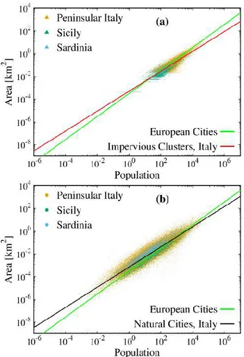
Figure 3 shows A-P relations calculated from the two methods, in a log-log scale as in Fig. 1. In both Fig. 3 (a), corresponding to the imperviousness method, and Fig. 3 (b), for natural cities, we show separately the (P, A) data points for peninsular Italy, Sicily and Sardinia. The straight lines, instead, are linear fit of the merged data sets. Both boxes also contain the linear fit for European cities (green curve), also shown in Fig. 1.

One can immediately appreciate that the two methods provide substantially different results, as far as the distribution of data points is concerned. In the case of Fig. 3 (a), corresponding to cities in Fig. 2 (a), data not only have a lower limit for the area, 400 m2_{, dictated by the resolution of the imperviousness layer,} they also show peculiar patterns, which are specific of the three distinct sub sets and can hardly be explained with simple arguments. On the other hand, in the case of Fig. 3 (b), corresponding to cities in Fig. 2 (b), data nicely distribute on the (P, A) plane, hinting to a linear correlation [4]. In this case, some patterns seem to emerge as well; however, they mostly emerge as collinear structures to the overall linear fit. Moreover, they seem

(18)

Figure 3. A-P relations from the two different approximations to delineate cities considered in this work, compared to results for municipalities (black and red curves). (a): cities delineated as disjoint clusters in the imperviousness layer; (b) natural cities (after Ref. [4]). A comparison of the geographical distributions of the two results, for Sicily, is in Fig. 2. Data points consist of three subsets, but the linear fits correspond to the aggregate data set. Green curve: fit to (P, A) data of European cities, from an independent data source, as in Fig. 1.

to exist only in the Sicily and Sardinia sub sets, suggesting some bias might occur for delineation of natural cities in smaller areas. In conclusion, we gave proof that a data-driven method for delineating cities such as natural cities, adopted in this work and in Ref. [4], represents an objective method for city delineation. The method provides advantages with respect to the delineation of cities by means of imperviousness products, as far as area-population scaling relations are concerned.

REFERENCES

[1] Fang, C., D. Yu, 2017. “Urban agglomeration: An evolving

concept of an emerging phenomenon”. Landscape and Urban

Planning 162, 126–136. DOI:

10.1016/j.landurbplan.2017.02.014

[2] United Nations, 2018. “The world’s cities in 2018”.

Department of Economic and Social Affairs, Population Division. Data booklet, ST/ESA/ SER.A/417

[3] Batty, M., 2018. “Inventing future cities”. The MIT Press, Cambridge, MA, USA. 304 pp. ISBN: 9780262038959

[4] Alvioli, M., 2020. “Administrative boundaries and urban areas in Italy: a perspective from scaling laws”. Landscape and Urban Planning (in press)

[5] Bettencourt, L., 2013. “The origins of scaling in cities”.

Science 340, 1438-1441. DOI: 10.1126/science.1235823

[6] Barthelemy, M. et al., 2013. “Self-organization versus

top-down planning in the evolution of a city”. Scientific Reports 3, 2153. DOI:10.1038/srep02153

[7] Arcaute, E. et al., 2015. “Constructing cities, deconstructing

scaling laws”. Journal of the Royal Society Interface. DOI: 10.1098/rsif.2014.0745

[8] Cottineau, C. et al., 2017. “Diverse cities or the systematic paradox of urban scaling laws”. Computers, Environment

and Urban Systems 63, 80-94.

DOI:10.1016/j.compenvurbsys.2016.04.006

[9] Steidl, M. et al., 2016. “Copernicus Land Monitoring Service - High Resolution Layer Imperviousness”. Technical Report version 1 of 985 2018-12-21. European Environment Agency. https://land.copernicus.eu

[10] Lu, D. et al., 2014. “Methods to extract impervious surface areas from satellite images”. International Journal of Digital Earth 7, 93-112. DOI: 10.1080/17538947.2013.866173

[11] Ma, D.et al., 2018. “Why topology matters in predicting

human activities”. Environment and Planning B: Urban

Analytics and City Science 0, 1-17. DOI:

10.1177/2399808318792268

[12] Thomas, I. et al., 2018. City delineation in European applications of LUTI models: review and tests. Transport Reviews 38, 6-32. DOI: 10.1080/01441647.2017.1295112

[13] Bettencourt, L., G. West, 2010. “A unified theory of urban

living”. Nature 467, 897 912-913. DOI: 10.1038/467912a

[14] Rozenfeld, H.D. et al., 2009. “The Area and Population of

Cities: New Insights from a Different Perspective on Cities”. Working Paper 15409. National Bureau of Economic Research. DOI: 10.3386/w15409

[15] Jiang, B., X. Liu, 2012. “Scaling of geographic space from

the perspective of city and field blocks and using volunteered

geographic information”. International Journal of

Geographical Information Science 26, 215-229. DOI: 10.1080/13658816.2011.575074

[16] Jiang, B., Y. Miao, 2015. “The evolution of natural cities from the perspective of location-based social media”. The

Professional Geographer 67, 295-306. DOI:

10.1080/00330124.2014.968886

[17] Jiang, B., 2018. “A topological representation for taking cities as a coherent whole”. Geographical Analysis 50, 298-313. DOI: 10.1111/gean.12145

(19)

An optimization of triangular network and its use in

DEM generalization for the land surface segmentation

Richard Feciskanin

§

_{, Jozef Minár}

Faculty of Natural Sciences Comenius University in Bratislava Ilkovičova 6, 842 15 Bratislava, Slovakia

§ _{richard.feciskanin@uniba.sk}

Abstract—Appropriate ge ne ralization of digital e le vation model (DEM) is important for the land surface segmentation. We tested some me thods of ge ne ralization base d on irre gular triangular ne tworks. Base d on the the ory of an optimal triangle for (land) surface re pre sentation, suitable me thods simplifying triangle ne tworks have be e n ide ntified. The quadric error metrics

simplification algorithm was use d to ge neralize surface mode ls. It

be longs to the de cimation algorithms de ve lope d in computer graphics, howeve r the u se of it for land surface mode ling is rare. Suitability of the me thod for the land surface se gmentation was e valuated for a varie ty of mode ls cre ated at different ge neralization le ve ls. Numerical e xpression of the concentration of the third-order parame te r values (curvature changes) around z ero (K0) was used as an indicator of the suitability. The hypothesis that the affinity of higher-order variables to a constant value should be significantly higher for re al land surface s with e le mentary forms than for mathe matical surfaces was confirmed. The re sulting K0 values are significantly lowe r in the artificial surface than in the re al surface mode l, howeve r only to a threshold limit of ge neralization.

I. INTRODUCTION

The question of scale and resolution is very important in geomorphological mapping. One of the major issues of quantitative modeling and analysis of the land surface is filtering to denoise, generalize, and decompose DEMs into components of different spatial scales [1]. When a coarser analytical scale is required, the original finer-resolution DEM needs to be generalized or simplified to reduce data redundancy [2].

A resampling method is one of the most widely used methods for DEM generalization, which requires averaging the neighboring cells of a high-resolution, square-grid DEM into a series of lower-resolution data sets. This method will inevitably have a peak-clipping and valley-filling smoothing effect [3]. Other groups of grid-based DEM generalization methods include wavelet transform, morphology-based, and drainage-constrained methods, each of them with its own difficulties [4].

The polynomial least squares fitting method with a changing calculation window size was used to generalize gridded data for hierarchical land surface segmentation in [5]. In this paper, we present the use of generalized triangular irregular networks (TIN) with different level of details for the same purpose. TIN allows to simplify the detailed model so that the resulting model retains as much information about the shape of the modeled surface as possible. The spatial structure of the TIN can represents the modeled surface very efficiently and yet accurately when designed with respect to the shape of the modeled surface.

Generalization algorithms developed for land surface modeling are mostly used to create a TIN model from a regular grid. These include traditional, still popular: The Fowler and Little algorithm [6], the Very important points algorithm [7], the Drop heuristic method [8]. Similarly, other algorithms presented in [9-12, 4] use various techniques to find the most appropriate (important) points for describing the land surface.

Generalization algorithms based on TIN are more widespread outside the land surface modeling domain. They are especially widespread in the computer graphics. In contrast to the algorithms mentioned above, they primarily focus on the overall shape fidelity of the simplified model. [13] evaluated simplification methods in computer graphics as mature almost two decades ago. Unlike grid-based method, TIN-grid-based methods from computer graphics are exceptionally used in the land surface modeling.

II. METHODS A. Optimal triangle

When optimizing the triangle network, we start from the theoretical assumption of an optimal triangle. [14] defines an optimal triangle whose plane has the same normal as the land surface at its centroid. A simpler but sufficiently precise description of this relationship will allow the replacement of part of the land surface with an osculating paraboloid with a vertex on land surface at the triangle centroid: Then it follows from the

(20)

above condition that the plane of the optimal triangle is parallel to the tangent plane of the surface (osculating paraboloid) at the triangle centroid (Fig. 1). The intersection of the triangle plane and the paraboloid is the same as Dupin indicatrix [15]. Consequently, the optimal triangle is one whose centroid lies in the center of the intersection conic. This can only be achieved in the case of an ellipse. The intersection is a circumscribed ellipse of a triangle centered in its centroid, known as the circumscribed Steiner ellipse. From the all circumscribed ellipses of the triangle, Steiner ellipse has the smallest area. It confirms the desirability of the approach. In places where Dupin indicatrix is not an ellipse, the condition cannot be fulfilled without deviation.

Figure 1. Optimal triangle representing land surface. The plane of the triangle

PiPjPk is parallel to tangential plane of the land surface in the point Pts at the

triangle centroid Ts. ns, nts – triangle normal and normal to surface at Pts are

identical. Isolines of height difference between the plane of the triangle and the land surface are shown.

[16] came to the same relationship, he defined the optimum ratio of triangle (ρ) replacing the quadratic surface as:

𝜌 = √𝜆2

𝜆1 (1)

where λ1 and λ2 are eigenvalues of Hessian of elevation function z = f(x, y). [17] defines a triangle aspect ratio as the ratio of the

principal axes of the ellipse with the smallest area that passes through the triangle vertices. Although not explicitly s tated, the authors deal with the circumscribed Steiner ellipse.

B. Simplification algorithms

We have identified simplification methods whose optimization conditions are in accordance with the above characteristics. These are the quadric error metrics simplification (QEMS) method presented in [18] and the memoryless simplification (MS) method introduced in [19]. Both methods were developed primarily for computer graphics, however they are also suitable for use in terrain modeling. [4] directly mention the QEMS method as a method for terrain simplifying, although they do not use it.

Both methods belong to the category of decimation methods. They use edge contraction to simplify the model's geometry. When contracting an edge, its two end points V0 and V1 are merged into a new vertex V. Condition for placing a new vertex is crucial. The final model consists of vertices that are not in the original data set. It allows to better maintain the local shape and has the ability to minimize the impact of random errors in the input data. The order of edges in edge list for contracting is determined by weighting of edge contraction. The contraction is repeated until the target condition is reached – most often the number of elements in the model.

The QEMS algorithm determines the edge contraction weight based on the value of the sum of the quadratic distance of the new vertex V from the individual planes of the triangles with the original merged vertices V0 and V1. New vertex location is in the smallest quadratic distance from the planes of triangles with the vertices V0 and V1. An example of one contraction step is shown in Fig. 2. In the MS method, the algorithm uses the sum of tetrahedron volumes that arise from the surrounding triangles by shifting the original vertices V0 and V1 to a new vertex V and an additional condition of preserving the volume.

Figure 2. Edge contraction and new vertex localization in quadric error

metrics simplification in 2D.

[17] showed that the aspect ratio, which is based on minimizing the quadric error, corresponds to the optimum ratio (1). Eigenvalues λ1 and λ2 are the extremes of principal normal curvature κ1 and κ2 and thus λ1 = κ1, λ2 = κ2. Extremal curvatures κ1 and κ2 correspond to the principal axes of Dupin indicatrix [17]. [20] presents that objective function for a new vertex localization

(21)

in MS bears a great deal of similarity to the quadratic form in the QEMS algorithm. The difference is only the weight of the triangle, they use squared value and absolute value of triangle area, respectively. This confirms that the above approach and so these methods use the same characteristics of the optimal triangle. The QEMS method we used to generalize the surface models. C. Testing triangle networks

Third-order morphometric variables were used to describe the suitability of a triangular network for land surface segmentation. Third-order variables may be used for confirmation of land surface affinity to constant values of second-order variables, that is a precondition of existence elementary forms suitable for geomorphological mapping [21]. A quantile-based measure of kurtosis (K0) presented in [21] was used as a numerical expression

of concentration of data around zero 𝐾0=

𝑥̃95− 𝑥̃5

𝑥̃0+5− 𝑥̃0−5 (2)

where x̃95 and x̃5 are percentiles representing the spread of the set

disregarding extreme values and x̃0+5 and x̃0−5 represent the fifth

percentiles on the right and on the left from the zero value. The values of slope line (s) and contour line (c) changes of profile curvature (kn)s and tangential curvature (kn)c denoted (kn)ss, (kn)sc, (kn)cc, (kn)cs were used.

We have determined the partial derivatives up to the third order for each vertex (except borders) and triangle centroids of the optimized triangular network based on the fourth order polynomial least square fitting. The input to the least square fitting were 3-ring neighborhood vertices. We calculated the summary characteristic K0 from the determined (kn)ss, (kn)sc, (kn)cc, (kn)cs values. This calculation was performed repeatedly for generalized models at different degrees of generalization.

[21] presents the hypothesis: The affinity of higher-order variables to a constant value should be significantly higher for real land surfaces with elementary forms or other structures than for mathematical surfaces. To confirm this, the same calculation of K0

was made on generalized models of the artificial surface. III. RESULTS AND DISCUSSION

The basic DEM of the surveyed area was created from a photogrammetric mapping in the form of a grid of 166×163 (27058) cells with a resolution of 2 meters. It represents an area located on the west of Bratislava, Slovakia, around the hill of Slovinec. The artificial surface model was calculated for 241×241 (58081) points based on a mathematical formula (trigonometric polynomial) with a fictitious 5 meters resolution.

The nodes of the regular grids form the vertices of the initial triangular networks. Initial TIN was generalized to more than 100

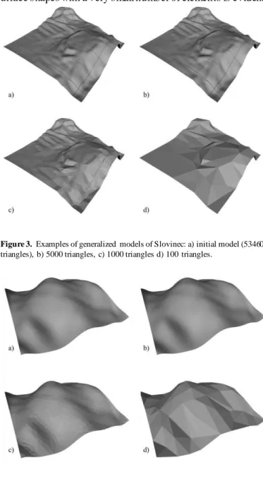
levels up to last 30 (40 in artificial surface) triangular faces. The selected generalization levels of the models are shown in fig. 3 and 4. The ability of the algorithm to capture the most important surface shapes with a very small number of elements is evident.

Figure 3. Examples of generalized models of Slovinec: a) initial model (53460 triangles), b) 5000 triangles, c) 1000 triangles d) 100 triangles.

Figure 4. Examples of generalized artificial surface models: a) initial model (115200 triangles), b) 5000 triangles, c) 1000 triangles d) 100 triangles.

The calculated values of K0 from the set of changes of curvature

(kn)ss, (kn)sc, (kn)cc, (kn)cs in each model are shown in fig. 5.

(22)

Figure 5. Values of K0 for each types of curvature changes in the whole range

of generalization.

The artificial surface has much lower values of K0 up to

generalization 100 – 200 triangles excluding (kn)cc (~700 triangles). It points to existence of elementary forms with affinity to constant value of (kn)s and (kn)c and/or their parent variables – slope, aspect and altitude. Generalizations with < 200 triangles make artificial and natural surface equal in light of K0. Instability

of moment based K0 (strong dependence on random values) for

small datasets can be one reason. An artificial facets (surface of particular big triangles) is another possible reason of convergence and extremums of both (artificial and natural) K0 curves.

IV. CONCLUSIONS

The optimization of triangular network by QEMS method (used nearly exclusively in computer graphics till now) can be effectively used for generalization of DEM. K0 index can be

suitable for determination of generalization levels optimal for land surface segmentation only to a certain level of generalization, given by approach of K0 curves of artificial and natural surface.

ACKNOWLEDGMENT

This work was supported by the Slovak Research and Development Agency under contract APVV-15-0054.

REFERENCES

[1] Florinsky, I. V. & Pankratov, A. N., 2016. “A universal spectral analytical method for digital terrain modeling”. Int. J. Geogr. Inf. Sci. 30, pp. 2506– 2528.

[2] Zhou, Q. & Chen, Y., 2011. “ Generalization of DEM for terrain analysis using a compound method”. ISPRS J. Photogramm. Remote Sens. 66, pp. 38–45.

[3] Chen, Y., Wilson, J. P., Zhu, Q. & Zhou, Q., 2012. “Comparison of drainage-constrained methods for DEM generalization”. Comput. Geosci. 48, pp. 41– 49.

[4] Wu, Q., Chen, Y., Wilson, J. P., Liu, X. & Li, H., 2019. “ An effective parallelization algorithm for DEM generalization based on CUDA”. Environ. Model. Softw. 114, 64–74.

[5] Minár, J., Minár, J. Jr. & Evans, I.S., 2015. “ Towards exactness in geomorphometry”. In Geomorphometry 2015 Conference Proceedings, Edited by: Jasiewicz, J., Zwoliński, Z., Mitasova, H. and T. Hengl, Adam Mickiewicz University in Poznań, Poland.

[6] Fowler, R. J. & Little, J. J., 1979. “ Automatic extraction of Irregular Network digital terrain models”. ACM Comput Graphics 13, pp. 199–207. [7] Chen, Z.-T. & Guevara, J. A., 1987. “ Systematic selection of very important

points (VIP) from digital terrain model for constructing triangular irregular network”. Auto Carto 8. pp. 50–56.

[8] Lee, J., 1989. “ A drop heuristic conversion method for extracting irregular networks for digital elevation models”. Proceedings of GIS & LIS’89. pp. 30–39.

[9] Fei, L. & He, J., 2009. “A three-dimensional Douglas-Peucker algorithm and its application to automated generalization of DEMs”. Int. J. Geogr. Inf. Sci. 23, pp. 703–718.

[10] Chen, Y. & Zhou, Q., 2013. “ A scale-adaptive DEM for multi-scale terrain analysis”. Int. J. Geogr. Inf. Sci. 27, pp. 1329–1348.

[11] Chen, Y. et al., 2016. “ A new DEM generalization method based on watershed and tree structure”. PLoS One 11, p. 23.

[12] Sun, W., Wang, H. & Zhao, X., 2018. “ A simplification method for grid-based DEM using topological hierarchies”. Surv. Rev. 50, pp. 454–467. [13] Luebke, D. P., 2001. “ A developer’s survey of polygonal simplification

algorithms”. IEEE Comput. Graph. Appl. 21, pp. 24–35.

[14] Krcho J., 1999. “ Modelling of georelief using DTM - the influence of point configuration of input points field on positional and numeric accuracy”. Geogr. časopis. 1999;51(3). pp. 225-260.

[15] Günther, F., Jiang, C. & Pottmann, H., 2020. “Smooth polyhedral surfaces”. Adv. Math. 363, p. 31.

[16] Nadler, E., 1986. “ Piecewise linear best l2 approximation on triangles”. In:

Chui, C.K., Schumaker, L.L. and Ward, J.D. (Eds.), Approximation Theory V, Academic Press, 499–502.

[17] Heckbert, P. S. & Garland, M., 1999. “ Optimal triangulation and quadric-based surface simplification”. Comput. Geom. Theory Appl. 14, pp. 49–65. [18] Garland, M. & Heckbert, P. S., 1997. “ Surface simplification using quadric error metrics”. Proceedings of the 24th Annual Conference on Computer Graphics and Interactive Techniques, SIGGRAPH 1997. pp. 209–216. [19] Lindstrom, P. & Turk, G., 1998. “ Fast and memory efficient polygonal

simplification”. Proceedings Visualization’98.

[20] Lindstrom, P. & Turk, G., 1999. “Evaluation of memoryless simplification”. IEEE Trans. Vis. Comput. Graph. 5 (2), pp. 98–155.

[21] Minár, J. et al. “ Third-order geomorphometric variables (derivatives): Definition, computation and utilization of changes of curvatures”. Int. J. Geogr. Inf. Sci. 27, pp. 1381–1402.

(23)

Detection of crevasses using high-resolution digital

elevation models: Comparison of geomorphometric

modeling and texture analysis

Olga T. Ishalina

a

, Dmitrii P. Bliakharskii

a

, Igor V. Florinsky

b, §

a

Department of Cartography and Geoinformatics Institute of Earth Sciences, St. Petersburg University

St. Petersburg, 199034, Russia b

Institute of Mathematical Problems of Biology

Keldysh Institute of Applied Mathematics, Russian Academy of Sciences Pushchino, Moscow Region, 142290, Russia

§

iflor@mail.ru

Abstract—The Vostok Station is the only Russian inland polar station in Antarctica. It is supplied by sledge and caterpillar-track caravans via a long sledge route. There are a lot of crevasses on the way. In this article, we compare capabilities of two techniques – geomorphometric modeling and texture analysis – to detect open and hidden crevasses using high-resolution digital elevation models (DEMs) derived from images collected by unmanned aerial survey. The first technique is based on the derivation of local morphometric variables. The second one includes estimation of Haralick texture features. The study area was the first 30 km of the sledge route between the Progress and Vostok Stations, East Antarctica. We found that, in terms of crevasse detection, the most informative morphometric variables and texture features are horizontal and minimal curvatures as well as homogeneity and contrast, correspondingly. In most cases, derivation and mapping of morphometric variables allow one to detect crevasses wider than 3 m; narrower crevasses can be detected for lengths from 500 m. Derivation and mapping of Haralick texture features allow one to detect a crevasse regardless of its length if its width is 2-3 pixels. Geomorphometric modeling and Haralick texture analysis can complement each other.

I. INTRODUCTION

There are five year-round operating Russian polar stations in Antarctica. Four of them – Bellingshausen, Novolazerevskaya, Progress, and Mirny Stations – are located on the coast of the Southern Ocean. The inland Vostok Station is situated at 3,488 m above sea level, at the southern Pole of Cold, near the Southern Pole of Inaccessibility and the South Geomagnetic Pole. Since 2007, the Vostok Station is supplied by sledge and caterpillar-track caravans via a 1430-km sledge route from the Progress Station.

The sledge route is intersected by a large number of crevasses formed due to glacier movements. The width of crevasses can vary from a few millimeters to tens of meters [1]. Crevasses hidden by snow bridges are extremely dangerous for researchers. Monitoring and timely detection of crevasses is important for the safety of participants of sledge and caterpillar-track caravans.

There are two main approaches for rapid detection of hidden crevasses: based and remote sensing ones. The ground-based approach involves studying a glacier with geophysical methods. Ground penetration radars are particularly applied, with antennas usually mounted in front of a vehicle. However, the safety and effectiveness of this approach is questionable [2]. The use of aerial and satellite imagery to detect open crevasses has high potential [1, 3, 4]. In this context, texture analysis of satellite data showed great efficiency. Low resolution of data is the main disadvantage of this approach [5].

In recent years, unmanned aerial systems (UASs) and UAS-derived products – orthomosaics and digital elevation models (DEMs) – have been increasingly used in glaciology [6]. In this article, we compare capabilities of two techniques – geomorphometric modeling and texture analysis – to detect open and hidden crevasses using UAS-derived high-resolution DEMs.

II. STUDY AREA

The study area is located south of the Progress Station, Princess Elizabeth Land, East Antarctica. We consider the first 30 km of the sledge route between the Progress and Vostok Stations (Fig. 1). From north to south, ice sheet elevations increase uniformly from 230 m to 850 m above sea level.

(24)

This area is characterized by a particularly large number of open and hidden crevasses, which makes the sledge route very dangerous. The width of crevasses varies from 0.5 m to 23 m. It was decided to detect crevasses in a buffer zone 1.5 km wide relative to the axis of the sledge route.

III. MATERIALS AND METHODS

An unmanned aerial survey (Fig. 1) was performed within the frameworks of the 62nd Russian Antarctic Expedition (austral summer 2016–2017); for details see [7]. For the study area, we obtained orthomosaics with a resolution of 0.08 m and DEMs with resolutions of 0.25 m, 0.5 m, and 1 m.

A hidden crevasse has a snow bridge, which makes it difficult to detect. However, a snow bridge can sink under gravity and, so, forms some sort of ditch. In fact, hidden crevasses are micro-landforms of the ice sheet topography. They should be manifested in a high-resolution DEM. Thus, to detect hidden crevasses, we previously used local and nonlocal morphometric variables derived from UAS-based DEMs [8].

On the other hand, crevasses can be reflected by changes in surface texture characteristics. Thus, to detect hidden crevasses, DEMs can also be processed by texture analysis techniques, in particular, using Haralick texture features [9]. Such approach was earlier utilized to reveal crevasses from satellite imagery [5].

To compare and validate these two approaches, we decided, first, to detect crevasses in areas where they can be visually recognized on orthomosaics or single images. For this purpose, 15 test crevasses were visually detected (Fig. 1). Length and approximate width of each crevasse were measured (Table 1).

It is not known a priori which particular morphometric variable will allow detecting crevasses. Therefore, for a site with two neighboring test crevasses (## 6 and 7), digital models for a set of fourteen local morphometric variables were derived from the DEMs, namely: slope, aspect, horizontal curvature, vertical curvature, mean curvature, Gaussian curvature, minimal curvature, maximal curvature, unsphericity curvature, difference curvature, vertical excess curvature, horizontal excess curvature, ring curvature, and accumulation curvature. For their definitions, formulas, and interpretations, see [10]. Both test crevasses were detected by only two morphometric variables, namely, horizontal and minimal curvatures. These two variables were used to reveal other crevasses at the further stages of the study.

These calculations were initially performed using the 1-m gridded DEM. Then, the DEMs with a resolution of 0.25 m and 0.5 m were tested. However, the experiment showed that these DEMs are marked by a high level of high-frequency noise resulted from photogrammetric processing of aerial images. These DEMs are not suitable for geomorphometric modeling [8].

Table 1. Characteristics of test crevasses (Fig. 1) Crevasse, # Length, m Width, m 1 123 1.5 2 77 1.5 3 883 2.0 4 191 3.0 5 170 5.0 6 913 7.0 7 476 8.0 8 117 0.5 9 99 0.6 10 644 5.0 11 247 7.0 12 501 2.0 13 300 3.0 14 155 0.6 15 139 2.0

Figure 1. Study area, zones of the UAS surveys, and location of crevasses.

(25)

Next, for the site with test crevasses ## 6 and 7, we derived a set of eleven Haralick texture features from the DEMs, namely: angular second moment (homogeneity), contrast, correlation, variance, inverse difference moment, sum average, sum variance, sum entropy, entropy, difference variance, and difference entropy. For their definitions, formulas, and interpretations, see [9]. In terms of crevasse detection, two Haralick texture features were the most informative, such as, homogeneity and contrast. These features are reciprocal, so only homogeneity was used in the next stages of the study.

To calculate the Haralick texture features, a gray level coincidence matrix (GLCM) is used [9]. GLCM is a table describing how often different combinations of brightness values or gray levels between adjacent pixels occur in an image in a certain direction.

To calculate the Haralick texture features, one should choose the following parameters:

• Size of a moving window. • Number of gray levels.

• Distance between compared pixels. • Direction.

The smaller is the size of features under study, the smaller should be a moving window. Elevation is a continuous variable, so elevation values should be re-coded into integer ‘gray levels’ before calculating the Haralick texture features from DEMs. If the number of gray levels is too small, the elevation range for each level will be too large. As a result, some topographic features will not be described because the corresponding pixels will have the same gray value. So, the number of gray levels should be as large as possible. A DEM has to be splitted into blocks, within which an elevation range does not exceed a certain value. In the calculation, each direction emphasizes topographic features of a certain orientation.

In this study, the size of a moving window was 3 × 3 pixels because crevasses are described by a small number of pixels. The distance between compared pixels was 1 pixel, that is, the values of neighboring pixels were compared. The number of gray levels was 256. We assumed that there could be different crevasse orientations, so all possible directions were considered. The 1-m gridded DEM was split into blocks so that an elevation range did not exceed 30 m.

Calculation and visualization of both local morphometric variables and Haralick texture features was carried out using QGIS software.

Table 2. Test crevasses detected (+) by different techniques Crevasse, # Horizontal curvature Minimal curvature Homogeneity 1 + 2 + + + 3 + + + 4 + + + 5 + + + 6 + 7 + + + 8 9 10 + + + 11 + + + 12 + + 13 14 15 +

IV. RESULTS AND DISCUSSION

In contrast to local morphometric variables, Haralick texture features are not so sensitive to the high-frequency noise and can be applied to DEMs with resolutions of 0.5 m and 0.25 m. As a result, the homogeneity map derived from the 0.25-m gridded DEM allowed us to reveal crevasses less than 1 m wide.

Figure 2 shows examples of crevasse manifestation on the orthomosaic and maps of elevation, horizontal curvature, and homogeneity. One can see no sign of two crevasses on the orthomosaic and elevation map, some traces of two crevasses on the horizontal curvature map, as well as clear image of two crevasses on the homogeneity map.

To compare capabilities of two techniques, we used the 1-m gridded DEM only. As a measure of technique effectiveness, we estimated the probability of test crevasse detection, that is, the probability is 1 if all 15 test crevasses are recognized by a technique.

Using the geomorphometric modeling, 9 of 15 crevasses were detected. The Haralick texture analysis allowed us to find 10 of 15 crevasses. As expected, all crevasses cannot be revealed by either technique (Table 2).

The probability of crevasse detection by the

geomorphometric modeling and the Haralick texture analysis is 0.60 and 0.66, correspondingly. Combination of two techniques leads to the probability of 0.73. Notice that among 15 test crevasses, 3 ones were less than 1 m wide (c.f. Tables 2 and 1). According to the first consequence of the sampling theorem [10], these crevasses cannot be detected using the 1-m gridded DEM: to keep the information on topographic features with typical planar sizes λ in a DEM, one should use the DEM grid size w ≤ λ/(2n), where n ≥ 2. Excluding these 3 test crevasses, the probability of the geomorphometric and Haralick detection