2016 Faculty Course Development Award
Measurement architectures for electric
systems
This work is an overview of what has been realized thanks to the grant received by the IEEE
Instrumentation and Measurement Society: the 2016 Faculty Course Development award.
As one of the winner of this award, I could deeply revise the content of the course I taught, buy new instruments for the didactic laboratory and show the students some new experiments.
The course program
The first operation I did, thanks to the award, is related to a deep modification of the program of the course I was teaching.
The old course was named “Digital processing of the measurement signals” and was divided into two main topics: the sampling techniques and the digital filters.
In particular, as far as the first main topic was concerned, the following topics were considered: the sampling theorem and, in particular, the sampling of periodic signals; the errors introduced by a non-coherent sampling (the leakage errors); the smoothing windows; the analog-to-digital conversion architectures (ADC), not only from the hardware point of view, but also considering the different contributions to uncertainty due to the possible non-idealities; the DSP architectures, analyzing their bandwidth and their possible different structures. On the other hand, as far as the second main topic was concerned, digital filters were considered as a specific example of DSP algorithms. In particular, digital filters were derived directly from the study of the dynamical systems. Then, FIR (finite impulse response) and IIR (infinite impulse response) filters were studied in details both from the theoretical point of view (stability/instability, causality, linear/non-linear phase, design…) and from the practical point of view (quantization of the parameters and architectures). According to the theoretical part, the practical laboratories of the old course were aimed at: acquiring a voltage signal; make experience with aliasing errors; implement the Fast Fourier transform of the acquired signal and make experience with the leakage errors; implementing FIR and IIR filters.
The new course, that I have taught since the 2016/2017 academic year, is named “MEASUREMENT ARCHITECTURES FOR ELECTRIC SYSTEMS”. The aim of is new course is to provide the students a deep understanding of how to develop measurement methods and techniques, based on intelligent instruments, to monitor and control the modern electric power systems, in a smart-grid scenario. In fact, even if based on well-assessed theoretical foundations, their knowledge is not always part of the background of the electrical engineer, although they have become more and more necessary nowadays, in the new smart-grid scenario. It is therefore important that the students have a deep knowledge of both the measurements theoretical basis and the modern measurement equipment.
According to this aim, some of the topics of the old course have been withdrawn and new topics have been added. In particular, the part related to the digital filters was not considered any longer, while the modern measurement structures and the modern measuring systems were added.
According to this, the program of the new course has become:
• the measurement systems based on the digital signal processing (DSP) techniques; • the sampling theorem and the aliasing error;
• the sampling of periodic signals;
• the errors introduced by a non-coherent sampling (the leakage errors); • the smoothing windows for mitigating the leakage errors;
• the analog-to-digital conversion architectures (ADC); • the errors introduced by the ADC;
• the effect of noise on the ADC behavior;
• the different structures for DSP architectures and their bandwidth; • the virtual instruments;
• the distributed measurement systems;
• the communication protocol of the distributed measurement systems, both on a local (LAN) and geographical (WAN) scale;
• the computer networks;
• the techniques for time synchronization of the different units of the distributed system; • the network time protocol and precise time protocol (based on IEEE Std. 1588v2: 2008) ; • the modern measuring systems for the most important electric system parameters:
spectral analyzers; power analyzers; PMU.
According to the new theoretical parts (with respect to the old course), further lab classes have been introduced.
First of all, a single voltage signal has been acquired and a virtual spectral analyzer developed. This first series of lab classes has allowed the students to deeply understand the implication of the sampling theorem and the analysis techniques in both domains (time and frequency).
Then, a voltage and a current signals have been acquired and a virtual power analyzer developed. This second series of lab classes has allowed the students to deeply understand how the sampling theorem influences the sampling conditions, according to the specific measurement algorithm.
Finally, a third series of lab classes has been dedicated to synchronization and synchronized measurements at different synchronization accuracies.
The course here described has been taught to the Italian students for two academic years. Conversely, from the next academic year, it will be taught in English, in the English track of the M. Sc. Level in Electrical Engineering at Politecnico di Milano (Italy). The name of the course will be “SMART MEASUREMENT ARCHITECTURES FOR ELECTRIC SYSTEMS”.
The didactic lab
The second operation I did, thanks to the received award, is to give birth to a new laboratory at the Dipartimento di Elettronica, Informazione e Bioingegneria (DEIB), at Politecnico di Milano: the laboratory for time synchronization and synchronized measurements.
In particular, the following material has been purchased: • 1 time server “MEINBERG LANTIME M1000S-IMS”; • 1 GPS antenna “MEINBERG”;
• 2 PTP slaves “MEINBERG PTP270PEX”;
• 1 switches “HIRSCHMANN RS20-0800T1T1SDAPHH08.0.”, compatible with the IEEE1588v2 Standard;
which allow to show the students some experiments related to the importance of synchronization.
Some demonstrations are also shown during a seminar about the time synchronization, hold by people from one of the most important Italian society devoted to time synchronization. During this seminar, it has been illustrated to the students the evolution of synchronization in the last 60-70 years, the operating principle of GPS antenna, the transmission of the timestamps and the PPS.
In the lab, the MEINBERG time server and the HIRSCHMANN switch have been installed, as shown in Fig. 1. The time server receives the GPS signal from the GPS antenna (Fig. 2). The time server provides a PTP signal [1], which is switched to six tables, thanks to the HIRSCHMANN switch (Fig. 1).
Fig. 2. GPS antenna, installed outside the building.
Actually, having purchased only two 2 MEINBERG PTP slaves, only two stations can receive the PTP synchronization signal out of the six available stations, since the received grant allowed to equip only these two stations.
Since all six tables have been wired to the switch, we plan to buy new MEINBERG PTP270PEX PTP slaves, as soon as new dedicated funds will be available.
All stations are also equipped with a signal generator, an ADC board (NI 9215) and, of course, a PC. Students have to learn how to program with National Instruments LabView. According to the available instrumentation, different levels of synchronization accuracy can be achieved in the lab:
• The two PCs with the PTP slave are able to read the time stamp sent by the time server directly by the PTP slaves. This means that the synchronization can be obtained with the PTP accuracy.
• The PCs which do not have a PTP slave are able to receive a time stamp through the net, according to the NTP protocol. Two different levels of accuracy can be achieved in this case.
o USE THE LOCAL REFERENCE. In this case, the time stamp sent by the time server is
read, through the net, by setting the IP address of the time server PTP signal. o USE AN EXTERNAL REFERENCE. In this case, an external time stamp is read,
considering an external server, such as, the one made available from INRIM, that is, the Italian National Metrology Institute.
• Finally, it is also possible not to synchronize our PCs.
In the following, one of the experimental classes dedicated to time synchronization is described.
A lab experience
Many different lab classes are experienced by the students of my course. However, since, as stated above, the IEEE grant has allowed to buy the necessary instrumentation for time synchronization, an experience related to this topic is here briefly reported. This experience has been called “Synchronization of a phasor” and the students are shown the impact of synchronization in the uncertainty affecting the measurement results.
A sinusoidal voltage signal is generated by a signal generator and acquired by two NI 9215 ADC boards in two different stations. The two boards are controlled through a dedicated Labview program, running on the PCs.
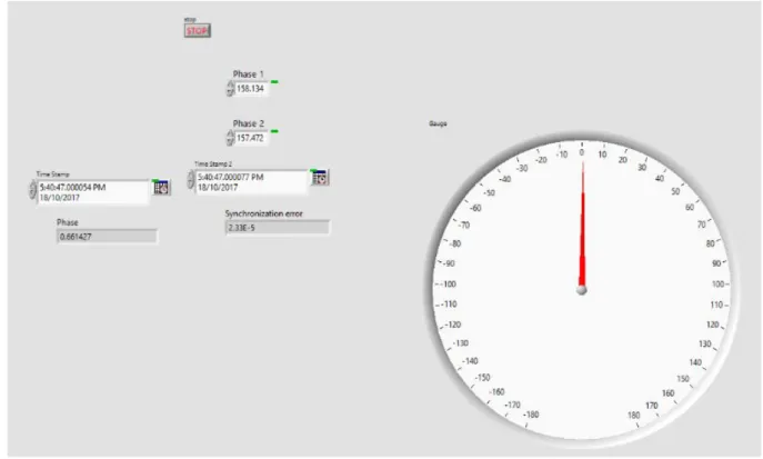
After acquisition, on both PCs, the acquired signal is elaborated, in order to obtain the voltage phasor. Fig. 3 shows one of the front panel of the dedicated VI, running on the two PCs. The figure shows: the sampling parameters, used for the sampling of the voltage signal; the graph of the acquired signal; the graph of the evaluated phasor, as well as the measured values of its module and phase angle.
Fig. 3. Front panel of the dedicated VI, for signal acquisition and evaluation of the signal phasor.
The measured values of the phase angle obtained in each measurement station are then sent to a master unit, through the National Instrument Data Socket communication protocol. The master unit receives the measured values of the phasors’ phase angles from the two measurement units and, for each couple of measured values, evaluates the difference, which should represent the phase difference between the two phasors. Fig. 4 shows the front panel of the dedicated VI at the master unit: the phase angles received, through the Data Socket communication protocol, from the two measurement stations are reported, as well as the evaluated phase difference.
Fig. 4. Front panel of the dedicated VI at the master unit.
In Fig. 4, a phase difference very close to zero is shown and this result is the one generally expected by all students. In fact, as far as they know, the two measurement stations are acquiring the same voltage signal and, therefore, they expect the same voltage phasor in the two stations and, consequently, a null phase difference between them.
On the other hand, this experience shows them clearly that this result is neither obvious nor immediate to be achieved.
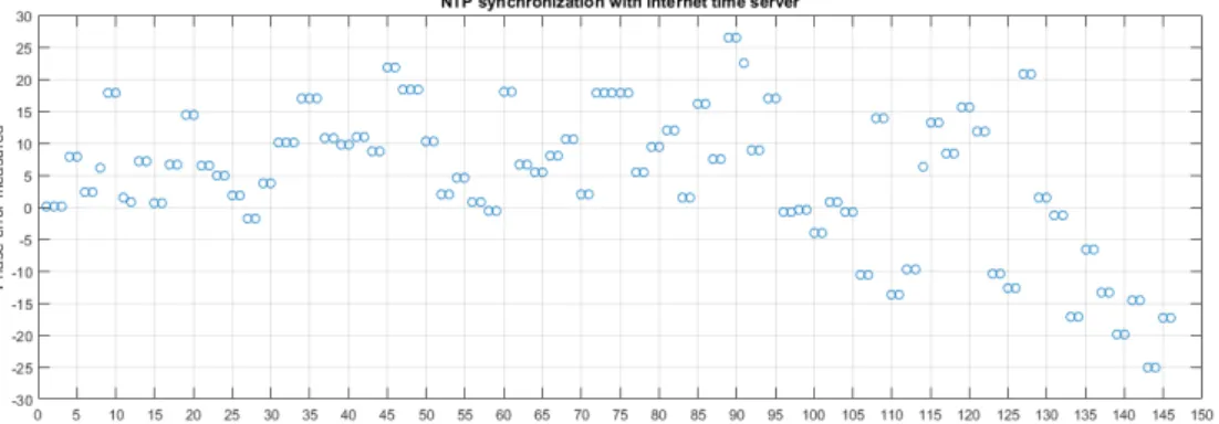
In fact, when a few hundreds of measured values of the phase differences are plotted, the results shown in Fig. 5 are obtained, which show a measured phase difference between -7 and -35 degrees. Therefore, some uncertainty contributions affect the measurement results. Of course, some contributions are due to the ADC board which introduce quantization errors and could also introduce gain errors or non-linearity errors. However, the dispersion of the plotted values clearly shows that some more important contributions are present. In particular, the figure shows that the uncertainty contributions affecting the measured values are of both random and systematic nature, since they distributes randomly around a mean value of about -23 degrees. These contributions are due to the lack of synchronization.
Fig. 5. Measurement of the phase difference between the two phasors evaluated at the measurement stations, when no synchronization is considered.
These first results are hence very useful to explain the students the importance of time synchronization. In fact, even if the two boards are acquiring the same sinusoidal signal, if, in each PC, the sampling conditions are simply set, without taking into account the exact time in which the acquisitions start, the acquisitions in the two boards are completely uncorrelated with each other. It follows that, when no synchronization is considered, it is quite uncommon to evaluate the same voltage phasor in the two different measurement stations, and a zero phase difference at the master unit. This is the reason of the obtained results, shown in Fig. 5.
On the other hand, if we want to draw the same phasor, in the two front panels of the VI running on the two measurement stations, we have to synchronize the two measurement stations, that is, to synchronize the signal acquisition in the two boards. This means that the two acquisition boards have to start the acquisition at exactly the same moment. Of course, this could be done very easily whether the acquisition boards on our tables had an external clock. Since our acquisition boards do not accept an external clock, a software synchronization is needed.
This can be achieved by setting exactly the time instant in which the acquisition (in the two measurement stations) must start. For instance, it is possible to read the PC clock and start the acquisition any time the read time stamp is “XX:XX:00” (hour:minutes:seconds). In this way, we start a new acquisition every one second.
This solution however can introduce a a systematic error in the measurement of the phase difference, if the clocks in the two PCs show a time delay. In order to avoid this, it is necessary to synchronize the two clocks between each other.
The more immediate one is to use the NTP protocol and refer to an external time server (for instance, INRIM, the Italian National Metrology Institute).
Under this assumption, the clocks of the two PCs are synchronized to the same reference and, therefore, they should show the same time stamps, at any instant. Therefore, both PCs should read time “XX:XX:00” (hour:minutes:seconds) at the same moment, so that the acquisitions start simultaneously.
This solution represents the cheapest possible one, since it only uses the net and no specific instrument is required. The obtained results are shown in Fig. 6.
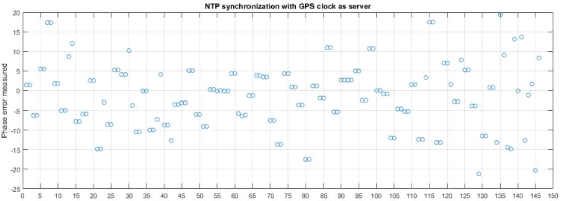
Fig. 6. Measurement of the phase difference between the two phasors evaluated at the measurement stations, when an NTP synchronization to an external clock is considered. Fig. 6 shows that, when the NTP protocol and an external reference is considered, the measured phase difference is evaluated in between -25 degrees and +30 degrees, with a mean value of about 5 degrees. With respect to the previous measured values (Fig. 5), we have obtained a greater variability, probably due to the net latency. Therefore, we have not improved too much our measurements and the measurement uncertainty is still quite high. A better accuracy can be obtained only by using dedicated instrumentation.
A solution to achieve a better accuracy is to use a local reference for time. Therefore, the NTP protocol is used, to synchronize the PC clocks to the Meinberg time server installed inside the laboratory.
Under this new assumption, the measurement results shown in Fig. 7 are obtained. The measured phase difference, in this case, is evaluated in between -21 degrees and +20 degrees, with a mean value of -1.5 degrees.
Fig. 7. Measurement of the phase difference between the two phasors evaluated at the measurement stations, when an NTP synchronization to the local clock (Meinberg time server) is considered.
With respect to the measured values in Fig. 5, it can be stated that NTP synchronization (in both cases of internal and external time reference) has allowed to drastically reduce the systematic contributions to uncertainty, but not to reduce the random ones. In fact, the dispersion of the measured values around the zero value (which is the ideal result) is still quite high. Therefore, better solutions must be exploited.
A better solution can be obtained when a synchronization with the PTP protocol is applied [1]. In this respect, the time stamp is not read from the internal PC clocks, but directly from the time server, through the PTP slave installed inside the PC's towers.
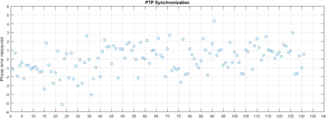
Under this assumption, the measurements shown in Fig. 8 are obtained. The measured phase difference, in this case, is evaluated in between -5 degrees and +5 degrees, with a mean value of -0.039 degrees.
Hence, with respect to the measured values in Fig. 5, it can be stated that PTP synchronization has allowed to drastically reduce both the systematic contributions to uncertainty and the random ones.
Fig. 8. Measurement of the phase difference between the two phasors evaluated at the measurement stations, when the PTP synchronization (Meinberg time server) is considered.
Conclusions
The students have shown to me a great interest in the new topics inserted in the course “MEASUREMENT ARCHITECTURES FOR ELECTRIC SYSTEMS", which they found to be modern and near to their everyday life.
They have also appreciated very much the laboratory experiences about synchronization and the seminar about the evolution of synchronization in the last decades.
This satisfaction has been possible also thanks to the grant received as a winner of the 2016 IEEE Faculty Course Development Award. Therefore, I would like to thank once again the IEEE Instrumentation & Measurement Society.
References
[1] IEEE Std. 1588-2008. IEEE Standard for a Precision Clock Synchronization Protocol for Networked Measurement and Control Systems.