UNIVERSITÀ DI PISA
Facoltà di Scienze Matematiche, Fisiche e Naturali
Corso di Laurea Magistrale in
Biologia Applicata alla Biomedicina
Curriculum Neurobiologico
Asymmetry of the Sylvian Fissure in Adolescent Onset Psychosis
Candidato: Sara Conti Relatori: Dott. Timothy Crow Prof. Mario Pellegrino
2
Contents
1. Abstract ...3
2. Introduction ...5
2.1 The phenomena of adolescent onset psychosis ... 5
A brief introduction on adolescent psychosis ... 5
Epidemiology ... 8
Classification of childhood psychoses and symptoms of adolescent psychoses ... 9
Risk Factors ... 12
2.3 Sylvian Fissure ... 18
2.4. MRI ... 23
2.5. BrainVisa ... 29
2.6. Aim ... 32
3. Materials and methods ... 33
3.1 Subjects ... 33 3.2 Image acquisition ... 35 3.3. Image Analysis ... 36 3.4. Statistical Analysis ... 41 4. Results ... 44 4.1. Gross Measures ... 44
4.2. Length of the Sylvian Fissure ... 47
4.3. Depth of the Sylvian Fissure ... 50
4.4. Correlations ... 53 5. Discussion ... 56 7. Appendix A ... 59 8. List of figures ... 67 9. List of tables ... 68 10. References ... 69
3
1. Abstract
The normal human brain is characterized by a pattern of gross anatomical asymmetry known as “torque” (a bias in width or volume from right frontal to left occipital). Contributing to the torque the Sylvian (lateral) fissure separates the frontal and parietal from the occipital and temporal lobes, and is reported to have a length bias to the left. The psychoses (schizophrenia and bipolar disorder) are a group of mental disorders characterized by a generally detrimental change in personality and a distorted or diminished sense of objective reality (i.g. they experience delusions and hallucinations). The psychoses occur in all populations with approximately uniform incidence and sex-dependent age of onset. This study aimed to test the hypothesis that individuals who develop psychosis in adolescence have atypical structural asymmetries of the Sylvian fissure.
We examined MRI scans from 32 adolescents (between 13 and 18 years old), divided as 17 controls and 15 patients. Baseline and follow-up magnetic resonance scans were collected through an imaging protocol with diffusion-weighted scanning on a 1.5-T Sonata MR scanner. All the brain scans were analysed through BrainVisa software. That allowed us to measure white matter, grey matter and CSF volumes. We found that grey matter was reduced in both the left (92,9%) and right (92,7%) hemispheres in patients compared to controls. Moreover in white matter (fibre tracts) we observed changes in laterality: controls were symmetrical whereas patients were more lateralised to the left (p = 0,020).
Then focusing on the SF and measuring total lengths, initially we observed no differences between patients and controls. To examine the SF in more detail, we adopted the Witelson and Kigar (1992) classification system that divides the Sylvian fissure into 3 segments: anterior, horizontal and vertical. The data were analysed with respect to a potential diagnosis x side x sex x length x depth interaction. In no analysis was sex found to be a significant variable. With respect to length, the vertical segment was found to be lateralized to the right (p < 0,001) and the posterior (anterior and horizontal together) to the left (p < 0,001). In both segments patients were found to have asymmetries that were reduced relative to controls. Depth asymmetries have so far been relatively neglected in schizophrenia. With BrainVisa we established that there are depth asymmetries of the SF and that these are reduced in individuals with schizophrenia. The core conclusion is that there is a reduction of the anatomical left and right asymmetry in SF in adolescents with schizophrenia (attested by changes in white matter, SF lengths and depths) consistent with the hypothesis that schizophrenia is a disorder of early neurodevelopment associated with anomalous cerebral
4
lateralization. The depth measures will facilitate discovery of the precise anatomical nature of the normal and deviant asymmetries.5
2. Introduction
2.1 The phenomena of adolescent onset psychosis
A brief introduction on adolescent psychosis
Psychosis is a group of severe mental disorders manifested in abnormal thinking and perceptions; people afflicted lose contact with reality.
It affects approximately 1% of the general population in the course of a lifetime, with onset typically in adolescence or early adulthood (Thornton and Seeman, 1988). The modern history of psychotic illness began with Morel in 1860, who coined the term démence précoce to refer to states of cognitive deficit that begin in adolescence. From the 1860s onwards, childhood insanity comparable to psychosis featured regularly in psychiatric publications and it was accepted that all forms of mental disease that occurred in adults could be present in children (Crichton-Browne, 1860). Then other psychotic syndromes were delineated in the late 19th century: Hecker (1871) distinguished hebephrenia (characterized by inappropriateness of emotional responses) and Kahlbaum described catatonia (with abnormal and stereotyped movements) in adolescents. At the end of the century (1887), Kraepelin proposed that both disorders of démence précoce and catatonia group together and he called these disease dementia praecox. It was a discrete mental illness, primarily a disease of the brain and particularly a form of dementia. The subtypes were catatonic, hebephrenic, paranoid and simple. Kraepelin chose the term dementia praecox, which means precocious deterioration of the intellect to distinguish this disorder from other forms of dementia (such as Alzheimer) which typically occur later in life. He thought that dementia praecox is a central nervous system disease involving very serious lesions of the cerebral cortex, the lesions are rather permanent or can only be regenerated in part, if at all. He believed that many other biologic abnormalities, including endocrinologic and genes cause schizophrenia.
The term “schizophrenia”, which comes from the Greek words “schizo” (split) and “phrene” (mind), was later introduced by Eugene Bleuler, a Swiss psychiatrist with the aim of referring to the lack of interaction between thought processes and perception.
6
Bleuler’s schizophrenia included a weakness of the association that brings about a loosening of mental links between mental contents. And he asserted that schizophrenia was a disorder of association between perceptions and thoughts. Bleuler estimated that 0.5 to 1% of schizophrenia cases had onset before the age of 10 and 4% before 15 years. He stated that “schizophrenia is not a puberty psychosis in the strict sense of the word, although in the majority of patients the sickness becomes manifest soon after puberty”. Moreover, unlike Kraepelin, Bleuler didn’t believe that schizophrenia led inevitably to deterioration and emphasized intrapsychic and psychosocial aspects.As far as concerns the history of psychosis, there has been a controversy whether it has been always existing or if it has recent origin (Hare, 1988). Finding evidence of psychosis in the past is quite difficult, because it wasn’t treated as a discrete entity but as a form of delirium, mania, melancholia, dementia, imbecility or idiocy. From the first half of the 20th century this view has changed, but the common view was that “madness” rarely occurred before puberty, although a small number of cases of insane children were described. From the 1860s it was accepted that all forms of mental disease that occurred in adults could present also in children (Crichton-Browne, 1860).
The first textbook on adolescent psychiatry was written by Hermann Emminghaus (Psychic Disturbances of Childhood, 1887); he described adolescent psychosis as “cerebral neurasthenia” and defined this disorder as “neurosis of the brain characterized by a reduction of cognitive (intellectual) abilities, mood changes, sleep disturbance and manifold anomalies of innervation with a subacute or chronic course and different states of outcome”.
Emminghaus was also the first to consider the psychosis as a disorder with a developmental perspective; indeed, epidemiological studies showed that the psychoses in children and adolescents rises across the age range.
In 1986 a study conducted in Sweden by Gillberg showed that 0,54% of all teenagers had been treated for a psychotic disorder but that the variation in prevalence was from 0.9/10,000 in 13-year-olds, rising to 17.6/10,000 in 18-year-olds. At a later stage, at age of 30 years old of the same sample, 35% of those with a diagnosis of schizophrenia in teenage had received the same diagnosis on repeated inpatient treatment in the 20-30 years’ age period.
7
An additional 13% were diagnosed as having chronic alcoholism and 13% were given diagnosis of paranoid reaction with Asperger syndrome, borderline personality disorder and atypical psychosis. Thus, 60% of the original group were still considered to have the schizophrenia more than 10 years after onset of psychotic symptoms in teenage. Moreover, all the adolescents with psychosis were still alive at the age of 30 and this result is in contrast with the risk of 5-15% suicide or accidental death directly due to psychosis reported in clinical studies (Werry et al., 1991). Only 20% of the group were relatively well recovered at the age of 30 years and were not undergoing psychiatric treatment. In a Canadian study (Maziade et al., 1996), which included 36 cases with adolescent onset schizophrenia, the outcome was even worse than in the study of Gillberg: about the 90% of the individuals received the same diagnosis at the age of 28. Other studies were conducted to predict the outcome of adolescent psychosis: Eggers and Bunk (1997) found a higher rate (25%) of complete remission; but 50% of their sample was judged to be in poor remission, to be chronically psychotic or to have developed a severe residual syndrome. In 1986, Zeitlin’s studies indicated a considerable continuity between psychosis in adolescence and adulthood: 90% of adolescents who had psychosis, still have it in their adult life.In conclusion, it has been demonstrated that only a small fraction (maybe less than 10%) of psychotic adolescent experience a “good” outcome.
8
Epidemiology
The study of the epidemiology of the psychotic disorders is not definitive yet, because the diagnostic criteria and the evaluation methods used in this kind of investigations are not always the same. Despite that, some epidemiologic information are proved (table 1). Schizophrenia has a ubiquitous epidemiologic distribution in the different geographic areas and in the different social status. Even the distribution between the sexes doesn’t reveal statistical differences.
The lifetime prevalence of this disorder is estimated around 0,5 – 1,5 % with an annual incidence of about 0,009 – 0,09 %.
Disorder Prevalence (%) Sex distribution
Schizophrenia 0,5 – 1,5 M > F*
Schizophreniform disorder 0,2 still to define
Schizoaffective disorder still to define M < F
Delusional disorder 0,05 – 0,1 M = F
Brief psychotic disorder still to define still to define
Table 1: Epidemiology of some psychotic disorders: lifetime prevalence in the general population and distribution among sex. * = slightly high incidence in male population.
9
Classification of childhood psychoses and symptoms of adolescent psychoses
Age and developmental stage are important criteria for the classification of childhood psychoses:
Early-onset psychoses: from birth to 3rd year;
Psychoses in early childhood: from 3rd to 5th year;
Late-onset psychoses: from 5th to 15th year;
Prepubertal psychoses: from 10th to 13th year;
Adolescent psychoses: from 14th to 20th year.
In this study we will focus on the last group of childhood psychoses, i.e. the adolescent psychoses. Psychoses manifested during adolescence may or may not have precursor symptoms in childhood (Rutter, 1967).
The symptoms of psychosis are usually divided into 2 classes: negative and positive symptoms. Negative symptoms are those that reflect the absence or diminution of behaviours, like: social withdrawal, poverty of speech, apathy, loss of interest. Positive symptoms, instead, are the psychotic symptoms “in excess” such as hallucinations, delusions and formal thought disorders. Actually, this distinction between positive and negative symptoms has been mostly used on psychosis in adulthood and rarely in adolescence. In fact, it has been shown that the symptoms vary according to age (Bettes and Walker, 1987): positive symptoms increase linearly with age, while negative symptoms occur most frequently in early childhood and late adolescence. The authors also found a few differences based on gender as well as a few correlations between symptoms and intellectual quotient (IQ): boys showed greater positive and negative symptoms than girls and children with high IQs showed more positive and fewer negative symptoms than low-IQ children.
Betters and Walker proposed 3 interpretations of their results.
1. Both symptoms may represent different psychiatric conditions with different underlying causes. (Crow T.J., 1980)
2. Both symptoms may be associated with different stages of the course of schizophrenia: for example, negative symptoms could be associated with advanced stages of the disorders. This interpretation, however, doesn’t explain the simultaneous increase of both the symptoms during adolescence.
3. It may be that the clinical manifestation of psychosis in the vulnerable children varies as a function of environmental demands and of characteristics of the individuals. Positive symptoms, in particular those that are based on ideational excess (paranoia, delusions, grandiosity) may increase as cognitive capacity increases. This would explain the linear increase in positive symptoms with age and the lower rate of positive symptomatology in low-IQ children.
10
In 1991 Remschmidt investigated the course of positive and negative symptoms during inpatient treatment. A comparison of positive and negative symptoms revealed a reduction of the number of symptoms with time but also a symptom shift in the direction of negativity. An interpretation is that at the beginning the negative symptoms could be hidden by positive symptoms and probably become evident after the disappearance of positive symptoms due to neuroleptic therapy (Angst et al, 1989). Another interpretation is that a high proportion of the patients become chronic. This study, in conclusion, demonstrates that the concept of positive and negative symptoms can also be used in adolescent psychosis and that they are dynamic symptoms that change during treatment and the course of the disorder. About 50% of adolescents with psychosis show an uncharacteristic symptomatology in their premorbid personality (Stutte, 1969). They are shy, introverted, sensitive, anxious and withdrawn. It is still unclear whether these personality characteristics directly predispose the adolescents to psychosis or whether they enhance their vulnerability. Psychosis begins with the first sign, no matter what type (positive, negative or non-specific), indicative of the disorder and is followed by the first negative and first positive symptom, the latter marking the end of the prodromal phase (early symptoms and signs of an illness that precede the characteristic manifestations of the acute, fully developed illness). According to a study of Heiden and Häfner (2000), in 77% of all cases the first sign of the disorder appeared before the age of 30, in 41% before the age of 20 and in 4% as early as before the age of 10. The main period of risk for the onset of psychosis went from ages 15 to 30 years, thus coinciding with the main period of social achievement in life. At 68% the insidious type of onset (earliest continuous sign of the illness more than one year before maximum of psychotic symptoms) was most frequent. The acute type (maximum of psychotic symptoms within one month after earliest sign of the disorder) was observed in 18% and the subacute type (earliest sign more than one month but less than one year before the maximum of psychotic symptoms) in about 15%. In 73% of all cases, psychosis began with a negative or a non-specific symptom and only in 7% with a positive symptom. In 20% symptoms of both categories appeared more or less simultaneously, that is, within the same month. From the 232 patients of the first episode sample, only 27% showed no prodromal phase. When asked for the first ever symptom, 19% of the patients reported restlessness and depression. Anxiety and troubles with thinking and concentration were rated next with some 18% and 16%, respectively, followed by worrying, lack of self-confidence and energy. In total, this finding indicates that psychotics tend to develop symptoms associated with a risk of social impairment as soon as onset has occurred and, thus, well before the first psychotic episode and first admission take place.11
Also between ages 13 and 18 years there is a decline in cognitive performance, especially in the verbal ability. This decline (except for the bipolar disorders) is a significant predictor of later psychoses and is a stronger predictor of later psychosis than poor verbal ability at age 18 years alone (Dalman, 2013).In the long run the clinical picture of psychosis changes: while during the first years positive symptoms, like delusions and hallucinations, will dominate, later in the course the symptomatology becomes more inconspicuous with negative and unspecific symptoms taking centre. Moreover, in contrast to the adult manifestation, the early manifestation of schizophrenia in adolescence still carries a particularly poor prognosis.
Onset of psychosis may be associated with abnormal adolescent neurodevelopment: epidemiological investigation has estimated that approximately 18% of adult schizophrenia patients experience initial onset of psychosis before being 18 years old (Hafner et al., 1993). These early-onset psychosis patients have increased neuroanatomical abnormalities (Rajji et al., 2009), greater cognitive impairment (Rajji et al., 2009), poorer medication response (Meltzer et al., 1997) and poor long-term outcome (Ballageer et al., 2005). Despite all the studies on this phenomena, why earlier onset predicts greater impairment is still unknown. According to Bramon et al., (2001) “Psychosis has a multifactorial etiology in which genes and early environmental brain insults interact to cause neurodevelopmental impairment and set pre-psychotic children on a trajectory of increasing deviance”.
However, the neurodevelopmental hypothesis has struggled to explain the timing of the onset of psychosis. The initial view was that an early brain abnormality interacts with normal events during adolescence. The latter potentially include hormonal changes, axonal myelination, and as well as environmental risk factors such as drug misuse and social stress (Broome M.R., 2005). In 1988 Watkins analyzed the precursors of psychotic symptoms in a group of 18 adolescents. He found out that the majority of the psychotic (schizophrenic) adolescents had significant developmental delays beginning during their infancy. 72% of the adolescents had deficits in language development or no language before 30 months year range. However, the frequency of language deficits decreased gradually across the 4 age ranges. These adolescents also showed problems in motor development, such as delays in reaching milestones and poor coordination (72%) and hypotonia (28%). The children with the most severe language problems had also acoustic-like symptoms (peculiar speech, lack of social responsiveness, self-mutilation) and they usually manifested schizophrenic psychotic symptoms during the 6 to 8 year range (one year early compared to the children with less language problem and no acoustic-like symptoms). During this age range, schizophrenic symptoms in 71% of these children were incoherence, loosening of associations and flat or inappropriate affect.
12
Rarely they showed delusions or hallucinations at that age; they started to appear at about 10 years old. These data indicate that there was a gradual, developmental increase of symptoms affecting social, cognitive, sensory and motor functioning in schizophrenic children.Risk Factors
For years lots of scientists have tried to understand which are the causes of psychosis; it has been attributed to many causes, styles of parenting, society, diet, unknown viruses and genes (Crow T.J. 2008), but since no theory is universally accepted it is better to talk about risk factors. Around 1980 some authors started thinking that psychosis was caused by a viral infection or by the exposure to influenza in the second trimester of pregnancy (Crow T.J. and Done D.J., 1992; Done D.J. et al. 1991), or another hypothesis was related to obstetric complications (Sacker A., et al. 1995). Moreover, for many years, researchers have suspected that schizophrenia is caused by a genetic abnormality. One of the earliest evidence that genes are important for schizophrenia was provided by Franz Kallmann (1946). He observed that the incidence of schizophrenia among parents, children, brothers and sisters with the disease was higher than that seen in the general population (1%). And the risk of developing schizophrenia in family members increases with the degree of biological relatedness to the patient: greater risks are associated with higher levels of shared genes (Gottesman, 1991). Kallmann started doing studies with twins and he found that monozygotic twins have a tendency for schizophrenia of about 50%, while dizygotic twins of 10%. But if schizophrenia was caused by genetic abnormalities than the tendency for twins to have the same illness would be nearly 100%. So, the 50% rate indicated that genetic factors are not the only cause, but because schizophrenia is five time more likely in identical than in fraternal twins, genetic factors must be important. Some scientists argue that the increased rate in identical twins might be explained in part by the psychological trauma of having a schizophrenic identical twin. To solve this problem, Leonard Heston and his colleagues studied adopted children whose biological parents suffered from schizophrenia and compared the rates of schizophrenia in these children to those of adopted children with normal parents. These studies found an increased rate of schizophrenia in the adopted children with schizophrenic parents compared to the ones with non-schizophrenic parents.
13
As mentioned before, another risk factor is age since in the majority of the cases schizophrenia starts between 15 and 30 with 2 incidence peaks correlated to gender: the first one regards males (14 – 24 years old) and the second one regards females (25 – 35 years old). Thus, earlier onsets with negative symptoms are commoner in males, later onset delusional illnesses are commoner in females, but diversity of form of illness increases with age to include bipolar and unipolar affective as well as paraphrenic illnesses (DeLisi, 1992). Moreover, the more persistent syndromes are commoner in males and acute transient illnesses in females (Marneros and Pillman, 2004). Season of birth is a risk factor as well: the incidence of schizophrenia is higher in people born in the last period of winter. The interpretation of this is still not clear since it could be the conceiving rather than the birth to determine the increased risk. Also neurodevelopmental factors are important in schizophrenia and this is demonstrated by the presence of neuropsychological abnormalities in children of patients with schizophrenia and by direct observations of the brain. In the 1970s groups of schizophrenics were found to have very slight differences in cerebral anatomy. The ventricles (which are large open structures lied deep in the brain and filled with cerebrospinal fluid) tend to be larger and this means that neurons and other brain tissue have smaller volumes (Johnstone et al., 1976). These kind of changes are most frequent in the left temporal lobe, in particular in an area important for language functions. These physical changes imply that schizophrenia is not a purely functional disorder. The changes were associated with reduction or loss of typical brain asymmetries, especially in temporal regions and also in frontal regions where the right side normally tends to be larger than the left (Luchins, 1979). Loss of asymmetry in schizophrenics was confirmed by post mortem studies (Brown et al., 1986).To sum up, table 2 (see next page) describes the main factors that need to be accounted for in any explanation of the phenomena of schizophrenia.
All these factors support the idea that psychosis is a disorder of humanity and may develop from a combination of brain chemistry, and genetic and environmental factors.
14
Kraepelin Bleuler Jablensky Wyatt et al. Crow MacDonald and Schulz KeshavanChapter 9 Chapters 8 and 9 First rank Features "Just the facts" Constraints "22 facts"
Incidence
Universal yes yes yes yes yes
Uniform Yes Yes yes yes yes
Onset
Age-restricted Yes Yes yes yes yes Yes yes
Sex-dependent Yes Yes yes yes yes Yes yes
Age of onset and sex > form of phychosis Yes Yes yes yes Yes
Symptoms
Childhood antecedents Yes Yes yes yes
Continua of variation Yes Yes yes yes yes Yes yes
Biological correlates
Ventricula enlargement yes yes Yes yes
Neuroleptics ameliorate symptoms yes yes yes Yes yes
Aetiology
Heritability Yes yes yes yes yes Yes yes
Absence of environmental factors Yes yes yes
Fecundity disadvantage yes
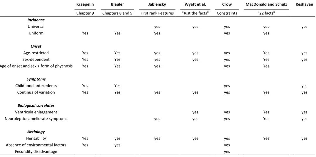
Table 2: Core features of schizophrenia commented on in Kraepelin (1919); Bleuler (1950); described as “first rank” by Jablensky (1988); specified as ++ or +++ by Wyatt et al. (1988) for reproducibility and primacy; designated by Crow (1995b) as constraints on theories of pathogenesis; included as 22 facts by MacDonald and Schulz (2009); listed by Keshavan et al. as “Just the facts” of schizophrenia.
15
2.2. Asymmetry of the brain
One of the early structural observations made about psychosis was the tendency for schizophrenic patients to deviate from the typical global frontal right and occipital left “twist” (Yakovlevian Torque) of the brain (Pearlson, 1997; Mackay, 1998; Cachia et al., 2008) (fig. 1). Local asymmetry changes were also found, primarily focused in the Perisylvian region of the brain: compared to the typical leftward bias of the Heschl’s Gyrus (HG) (Shergill et al., 2000; Dorsaint-Pierre, 2006) and the Planum Temporale (PT) (Shapleske et al., 1999; Horn et al., 2009), patients have demonstrated reduced asymmetry in both (Kwon et al., 1999; Oertel et al., 2010), although this has not been consistent (Barta et al., 1997). Different definitions of the structures and population age may account for this: some groups have suggested that asymmetry perturbations may be progressive rather than static (Toga and Thompson, 2003) and so cohort age and duration of disorder may be critical.
As perysilvian regions are associated with both language and auditory processing, these structural asymmetries have been argued to underline the functional lateralization, i.e. different hemispheric specialization, of these faculties. In fact, anatomically, the cerebral cortex is divided into frontal, temporal, parietal and occipital lobes, and these regions control thinking, language, movement, sensation, vision and other functions. The cerebral cortex is also divided in left and right hemispheres; the left hemisphere is normally dominant for language and logical processing, whereas the right hemisphere is specialized for processing spatial relations and for emotional control. This segregation of functions in the human brain, i.e. functional asymmetries in the human brain were initially thought to be uniquely human, reflecting unique processing demands required to produce and comprehend language. However, functional and structural asymmetries have been identified also in non-human primates and in many other species: for instance Japanese Macaques have a right-area advantage for processing auditory system or passerine birds produce song primarily under left-hemisphere control. Despite that, man, among all the animals, has considered to have the most asymmetric brain: asymmetry is the defining characteristic of the human brain (Broca, 1864). This concept was particularly underlined thanks to the anatomical discovery of asymmetry by Geschwind and Lewitsky in 1968: they did a study on post-mortem human brains and they found out an asymmetry in favor of the left hemisphere.
16
The first detailed description of functional asymmetry in the human brain was made in 1864 by a French neurologist Paul Broca. He found that there was a lesion in the left hemisphere in the post-mortem brain of a patient who couldn’t produce speech. This area of the brain, called Broca’s area, lies close to part of the so-called motor cortex of the brain associated with movements of the mouth. Broca claimed that language ability in the human brain is lateralized and suggested that the left-cerebral dominance for language might be attributable to earlier growth of the left hemisphere relative to the right.In 1874, there was another discover by a German neurologist Carl Wernicke, he found out that damage to a region of the left hemisphere could cause a type of aphasia that makes the individual unable to understand speech. This area is called Wernicke’s area and is located in the upper posterior part of the temporal lobe, around the junction of the temporal, parietal and occipital lobes.
Functional asymmetries in language processing zones correlate strongly with handedness, implicating the planum temporale and other areas surrounding the Sylvian Fissure: in language, articulate and formal aspects such as grammar are represented in 90 – 96 % right-handed population on the left (Pujol et al., 2002), whilst global aspects of language such as prosody and humor are represented on the right (Mitchell and Crow, 2005). This varies within the population, and handedness may be an indicator that is associated with language lateralization (Hatta, 2007) though this is relative and not absolute: in handed people, articulate language is left-lateralized only 70 % of the time (Josse and Tzourio-Mazoyer, 2004).
Thus, brain functional asymmetry is not limited to language ability; for instance, the right cerebral cortex regulates movement of the left side of the body and the left cerebral cortex regulates movement of the right side: more than 90% of the human population is naturally more skilled with the right hand which is controlled by the left hemisphere. So, many cognitive and motor functions, such as handedness, language, linear reasoning, numeric and arithmetic skills are often lateralized to one hemisphere. (The term “lateralization” is used to denote a function that is preferentially subserved by the right or the left side of the brain; for instance, language is commonly lateralized to the left hemisphere).
These structural asymmetry differences in the schizophrenic population have been argued to represent atypically lateralized function: a “nuclear” language deficit (Crow, 2000) which is in turn associated with other symptom in psychosis such as impaired speech processing (Stephane et al., 2001; Frith, 2005), disorganized speech (DeLisi, 2001) and even auditory hallucinations (Shergill et al., 2000; Catani el al., 2011).
17
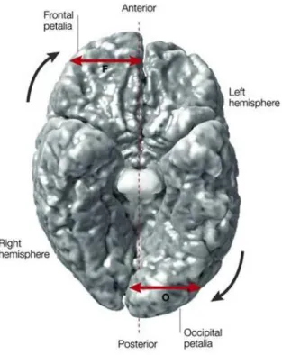
These observations do not themselves imply a causative role necessarily. However, correlations with severity of symptoms with extent of structural reduction (Oertel et al., 2010) and functional interactions in the Superior Temporal Gyrus (STG) (Horn et al., 2009) are suggestive. Furthermore, the discovery that non-affected, unimpaired high-risk family members have an intermediately lateralized HG phenotype (Oertel et al., 2010) suggests this may be a genetic endophenotype and specific-factor for psychosis (Oertel-Knöchel and Linden, 2011) rather than representing cognitive impairment in general as some groups (Leonard et al., 2008) have argued.Fig. 1: Schematic showing prominent asymmetries found in the gross anatomy of the two brain hemispheres.
Diagram adapted from Toga et al. (2003), derived from an in vivo magnetic resonance imaging scan in radiological view.
As showed in figure 1, there are noticeable protrusions of the hemispheres, anteriorly and posteriorly, as well as differences in the widths of the frontal (F) and occipital (O) lobes. These protrusions are known as petalias, which are a type of cerebral asymmetry, with greater protrusion of the surface of one hemisphere beyond that of the opposite hemisphere. The Yakovlevian torque is also observed, where the left occipital and frontal right is “twisted” in space and reported to be larger in size. This is not as prominent in the schizophrenic sample brain, which is matched to age and sex.
18
2.3 Sylvian Fissure
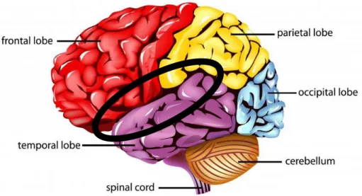
Subject of this work is the Sylvian fissure (SF or lateral fissure), which is the core of the Perisylvian Region. It is one of the primary fissures of the primate brain and separates (fig. 2) the frontal and parietal lobes (which lie above the fissure) and the temporal lobe (which lies below the fissure). Usually the primary fissures are formed by an infolding of the cortex, instead the SF results from uneven growth of the outer cortex relative to inner structures (Cunningham, 1892).
Fig. 2: The Sylvian Fissure. Figure adapted from www.wisegeek.com.
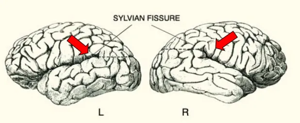
The SF reflects the local anatomical variation in the gyri and share an asymmetric trajectory and leftward bias (Rubens et al., 1976; Ono et al., 1990), suggesting SF morphology is also associated with lateralized function. For over a century, in fact, it has been known that the left and the right Sylvian fissures are typically asymmetric at the posterior end; in particular the right-hemisphere fissure curls upward more than the left one (Cunningham, 1982) (fig. 3).
19
Fig. 3: Asymmetries of the SF. The SF is typically longer and straighter in the left hemisphere than in the right hemisphere. Figure adapted from Geschwind N., Specializations of the human brain, Scientific American, June 1992, p.185.Moreover, the SF is typically longer in the left hemisphere than in the right hemisphere, leading to the suggestion that the temporal and parietal opercula are larger in the left hemisphere (Geschwind and Galaburda, 1987). Additional evidence for this theory comes from the finding that the height of the end-point of the SF is negatively correlated with the volume of the planum temporale: it shows a marked leftward volume asymmetry (Geschwind and Lewitsky, 1968) that is related to the degree of right-handedness.
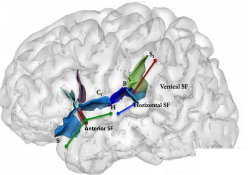
Asymmetries in the length of the SF have also been reported in the brains of infants, children and adolescent and they are similar to the asymmetries in the brains of the adults. This asymmetry has also been explored in schizophrenic patients, where they were atypically lateralized (Falkai et al., 1995; DeLisi et al., 1997; Sommer, 2001). This concept however has not always been demonstrated (Bartley et al., 1993), probably because it’s quite difficult to delimit the SF. Witelson and Kigar (1992) recognized this problem and devised a classification system that demarcated 3 segments to the SF based on well-defined landmarks: anterior (ASF), horizontal (HSF) and vertical (VSF) (fig. 4). When they analyzed length values in their cohort according to these definitions, they found 3 different relationships. The anterior-SF was symmetrical between hemispheres, whereas the horizontal-SF had a leftward bias and this was likely responsible for the majority of papers which reported a leftward bias. The vertical-SF however, had a rightward bias, and if these were not considered separately, these bias could cancel out (Table 3).
20
Figure 4. Schematic showing the right SF with the landmarks and three segmentations. Figure adapted from Witelson and Kigar, 1992.S: anterior edge; A: where the anterior ascending and horizontal ramus meets the main sulcus; H: where the transverse section of the Heschl’s Gyrus meets, or can be extended to the SF; B: the bifurcation point between S1 Posterior Ascending Ramus, and Posterior Descending Ramus; C1: point to which the central sulcus (CS) can be extended to the SF (more historic).
21
Witelson & DeLisi et Ono et Ide et al., Vannier et al., Falkai et al., Bartley et al., Rubens et al.,Kigar, 1992 al., 1997 al., 1990 1996 1991 1992 1993 1997
Method MRI MRI Post-Mortem Post- Mortem MRI, Polaroid
overlay MRI MRI Polaroid tracings
Anterior SH L = R L = R
Horizontal HB L > R L > R L > R* L > R
Vertical HS R > L R > L L = R R > L
Total S-S1 L = R L = R L = R*
A-B: L = R,
Other B-S2: L > R S-A: L > R, A-B: L > R A-C: L > R, A-B: L > R,
A-S1: R > L C1-B: R>L* PC-B: L > R Notes Sex intercations, large bias in female MRI slice thickness large: error margin Sulcus atlas Used straight, versus curved, lenghts MR and in vivo results werw comparable Coronal slices, did not control for bandedness Looked at control twins, versus patients Small sample size, no LH
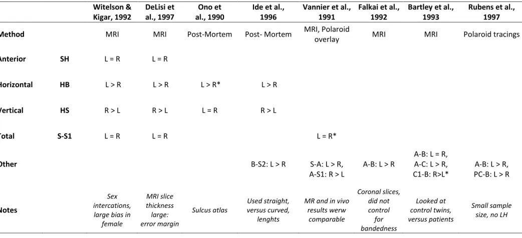
Table 3: Review of asymmetry results of different SF segments from both Witelson and Kigar (1992) and other studies. There are summarized the asymmetry results of Witelson and Kigar’s original cohort according to their landmark and classification system. Other studies which listed their measurements definitions with the raw data were also mapped onto the same classification to determine whether they were consistent across studies.
All samples are mixed (in gender, handedness) but healthy (all controls). Refer to Figure 4 for acronyms and landmark locations. Sometimes measurements were not given directly, but could be calculated by other given measures. These are denoted with an *.
22
These observations have the potential to explain discrepancies in SF reported lengths if they are robust, and so a wide range of studies were re-examined in Table 3 according to the classification and landmarks of Witelson and Kigar (1992) to see whether they were consistent across studies. Studies that were included had healthy control populations, clear anatomy boundary definition and enough raw measurement information to allow comparisons. From this, it would appear that most of the segment asymmetry relationships do seem replicated. It also demonstrates the large heterogeneity of measurement landmarks and measurement techniques.Whether this standardization can be applied for the work done in schizophrenic cohorts would be interesting to consider as previous work has used many different measurements so synthesis is difficult: Falkai et al (1995) found atypical lateralization in schizophrenic patients post-mortem according to A-B, whereas a discordant twin study failed to replicate this (Bartley et al. 1993), though they used the post-central sulcus aspect (A-PC1).
23
2.4. MRI
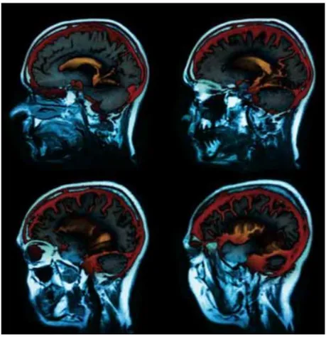
Magnetic Resonance Imaging (MRI) is a technique commonly applied in medical clinical and research practice to provide visualization of internal biological tissue structures (fig. 5).
Figure 5: Example of MRI images. Figure adapted from Stoddart A., Nature Milestones, 2008.
The main advantages of MRI are that it is not invasive, it does not use harmful radiations (non-ionizing radiations), it produces truly 3D images of high resolution with a high signal-to-noise ratio (SNR), and it’s versatile (which means that by changing the scanning parameters, can be generated images based on a variety of different contrast mechanisms).
24
As its name implies, MRI uses strong magnetic fields to create images of biological tissue; in particular to create images the MRI scanners use a series of changing magnetic gradients and oscillating electromagnetic fields, called a pulse sequence (Magnetic Resonance Imaging, TBI TECHNOLOGY News). Depending on their frequency, energy from the electromagnetic fields may be absorbed by atomic nuclei. MRI scanners are tuned to the frequency of hydrogen nuclei (that is the proton), which are the most common in the human body due to their prevalence in water molecules. After it is absorbed, the electromagnetic energy is later emitted by the nuclei and the amount of emitted energy depends on the number and type of nuclei present. In particular, the proton responds to applied magnetic fields by emitting characteristic radio waves. Each proton rotates around its axis, acting as a magnet with its own dipole. The protons in a magnetic field become aligned, while usually they are directed at random so the tissue has no net dipole. A second magnetic field formed by a radio frequency pulse is applied to the tissue and causes protons to start wobbling around their axes (this process is called precession). Precession creates a rotating magnetic field that changes in time and in the MRI it is this electric current that is measured. When the radio frequency pulse is turned off, protons in the tissue relax: the proton that were rotating together begin to fall out of synchrony with one another and their axes become aligned with the original magnetic field. MRI measures the rate of 2 relaxation processes characterized by time constants T1 and T2,where the relaxation is the mechanism that generates the contrast between different tissue in MRI (in fact, the difference in the physical properties of different tissue types is reflected in the relaxation time) (Fig. 6). These changes in the tissue takes place as the excited protons relax back to their lower energy state after the radio frequency pulse is turned off.
25
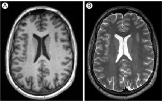
Figure 6: Images with different contrast: the same slice has been acquired both with T1 weighted (A) and T2weighted (B) contrast. Figure taken from Daducci A., 2009.
The relaxation component emphasized in the T1 weighted image represents the moment
when the protons realign with the original magnetic field; thus T1 records the time from the
cessation of the pulsed radio beam to the signal being emitted
.
The rate of this relaxation is influenced by non-excited molecules in the surrounding tissue. In a T2 weighted image isemphasized the falling out of synchrony of rotating protons; thus T2 measures the length of
the signal once the proton has un-flipped and released the signal. This phase occurs quite quickly and results from the loss of energy to spinning nuclei nearby. The relaxation time and the corresponding T1 and T2 time constants of the protons depends on whether they are
embedded in fat, white matter, cerebrospinal fluid, etc.
The ability to localize the signal in the 3-dimensional volume of the brain is accomplished by using magnetic field in which the strength of the field changes gradually along an axis. Applying gradients along 3 axes subdivides the tissue: one magnetic gradient is used to excite a single slice of the subject’s brain, 2 more gradients subdivide that slice into rows and columns.
26
MRI scanners have 3 main components: static magnetic field, radiofrequency coils and gradient coils which together allow collection of images:1. Static magnetic field: MRI uses strong static magnetic fields to align certain nuclei within the human body (usually hydrogen within water molecules) to allow mapping of tissue properties. This magnetic field is created through electromagnets, which generate their fields by passing current through tight coils of wire. The static magnetic field created by an MRI scanner is expressed in units of Tesla (one Tesla is equal to 10,000 Gauss). There are 2 criteria for a suitable magnetic field in MRI: homogeneity (or uniformity) and strength. The first is necessary in order to obtain images of the body that do not depend on which MRI scanner is used or how the body is positioned in the field. So, a homogeneous magnetic field is one that has the same strength throughout a wide region near the center of the scanner bore. A typical design for generating a homogenous magnetic field is a solenoid in which a coil of wire is wrapped tightly around a cylindrical frame. In order to fulfil the second criteria, it’s necessary generating an extremely large magnetic field injecting a huge electric current into the loops of wire. To generate this kind of field it’s requested an enormous electrical power and thus enormous expense: modern MRI scanners use superconducting electromagnets whose wires are cooled by cryogens (such as liquid helium) to reduce their temperature to near absolute zero. Coil windings are typically made of metal alloys such as niobium-titanium, which when immersed in liquid helium reach temperatures of less than 12 K (-261°C). At this extremely low temperature, the resistance in the wire disappears, thereby enabling a strong and lasting electric current to be generated with no power requirements and minimal cost. Combining the precision derived from numerical optimization of the magnetic coil design and the strength afforded by superconductivity, MRI scanners can have homogenous and stable field strengths in the range of 1 to 9 T for human use. Since maintaining a field using superconductive wiring requires little electricity, the static fields used in MRI are always active.
27
2. Radiofrequency coils (to collect MR signal): MR signal (the current measured in a detector coil) is produced by 2 types of magnetic coils, known as transmitter and receiver coils. These 2 coils generate and receive electromagnetic fields in at the resonant frequency of the atomic nuclei within the static magnetic field. An equilibrium state exists when a human body is placed in a magnetic field, because the net magnetization of atomic nuclei (hydrogen) within the body becomes aligned with the magnetic field. The radiofrequency coils send electromagnetic waves that resonate at a particular frequency, as determined by the strength of the magnetic field, into the body, perturbing the equilibrium state. This process is the excitation. When atomic nuclei are excited, they absorb the energy of the radiofrequency pulse; but when the radiofrequency pulse ends, the hydrogen nuclei return to the equilibrium state and release the energy that was absorbed during the excitation. The resulting release of energy can be detected by the radiofrequency coils, in a process called reception. This detected electromagnetic pulse defines the raw MR signal.3. Gradient coils (to provide spatial information in the MR signal): the ultimate goal of MRI is to generate an image and gradient coils provide the component necessary for imaging. The purpose of a gradient coil is to cause the MR signal to become spatially dependent in a controlled fashion, so that different locations in space contribute differently to the measured signal over time. Gradient coils are used to generate a magnetic field that increases in strength along one spatial direction. The spatial directions used are relative to the magnetic fields, with z going parallel to the main field and x and y going perpendicularly to the main field.
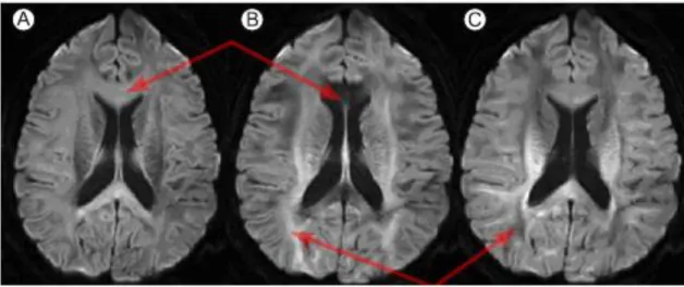
This study has been conducted using diffusion weighted imaging (DWI) (fig. 7) which is a form of MRI based upon the random Brownian motion of water molecules within a voxel (Le Bihan D., 1991). The movement of water molecules in biologic tissues is restricted because their motion is modified and limited by interactions with cell membranes and macromolecules. The DWI signal is derived from the motion of water molecules in the extracellular, intracellular and intravascular space (given a unit time, water molecules in the intravascular space will have a greater diffusion distance because of blood flow than those in the extracellular and intracellular spaces).
28
Diffusion-weighted sequences are made sensitive to diffusion by the insertion of two additional magnetic field gradient pulses (or diffusion gradients). The first of the two gradient pulses introduces a phase-shift that is dependent on the strength of the gradient at the position of the spin at t = 0. Before the application of the second gradient pulse, which introduces another phase-shift dependent on the spin position at t = ∆, a 180° radio-frequency pulse is applied to reverse the phase-shift induced by the first gradient pulse. As long as spins remain at the same location along the gradient axis between the 2 pulses, the net phase accumulation will be constant irrespective of their position and therefore they will return to their initial state. However, spins that have moved will be subjected to a different field strength during the second pulse and therefore will not return to their initial state but will experience a nonzero phase-shift. If all spins underwent the same net displacement, they would all undergo the same phase change, such that, although the phase had changed, the signal would remain coherent and there would be no concomitant drop in signal amplitude. Under the diffusion process, however, there is a distribution of displacements and thus a distribution of phases. This phase dispersion leads to a loss of coherence and therefore a reduction in signal amplitude. The wider the spread of displacements, the greater the loss of signal.Figure 7: Diffusion-weighted images obtained, for the same slice, with diffusion gradients oriented in the Inferior-Superior (A), i.e. through the plane, Left-Right (B) and Anterior-Posterior (C) direction, respectively. Figure taken from http://www.med.lu.se
29
2.5. BrainVisa
Brain morphometry has proven to be a powerful tool in identifying key points of many neurological and psychiatric disorders. Several studies have investigated the link between the changes in the brain morphology and certain diseases or disorders such as schizophrenia. One of the popular software packages for brain morphometry is BrainVisa.
BrainVisa 4.3.0 is a freely distributed software, written in Python language and can be downloaded from: http://brainvisa.info. It examines the cortical folding of the brain (Mangin et al., 2004.). In addition to the most common morphometry metrics, this program allows a sulcus-based morphometry (Condon et al., 2011). This is possible thanks to the automatic sulci recognition feature of the program which automatically identifies the sulci of each individual brain. Sulcus parameters (volume, depth, location and pattern) can then be computed for each sulcus.
This method differs from the other morphometrical analyses, because it quantifies both the surface area and mean depth of the sulci rather than relying only on the linear length of the outer contour of the sulcus. This is important because measures of the length, by themselves, may not capture all size dimensions of the sulci while with BrainVisa all dimensions of variability in organization (length, depth and surface area) are captured.
30
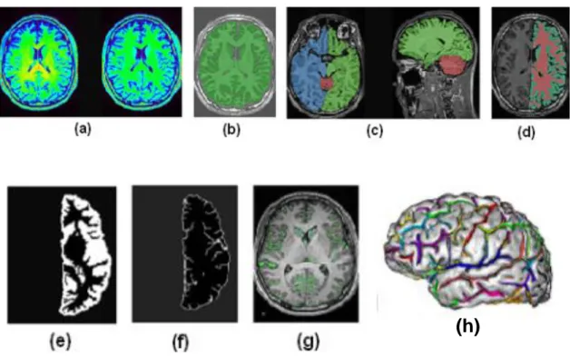
MR data has to be imported into BrainVisa (version 4.1) and the pipeline process of extracting the sulci from the cortex involves several steps (fig. 8), which can also be checked manually.Figure 8: Different steps of data pre-processing in BrainVisa.
To align the template brain according to the Talairach and Tournoux atlas, the anterior and posterior commissures are manually specified on the MRI at the intrahemispheric point. The first step is to correct the spatial inhomogeneities in the signal intensity in order to obtain a stable distribution of tissue intensities (a). Then, there is the histogram analysis which finds the peaks corresponding to grey matter, white matter and cerebrospinal fluid. At this point, using the information from this histogram analysis and removing skull and non-brain tissue, a mask of the brain is created (b). Cerebellum, left and right hemispheres are split (c) and segmented into grey matter, white matter and cerebrospinal fluid (d). This means that morphometric measures are calculated for every scan of each subject and the measurements are performed for each cerebral hemisphere independently. The morphometric measures are either global (brain tissue volume and global sulcal index) or sulcal (parameters that are calculated for each sulcus independently; i.e. sulcus surface and sulcus mean geodesic depth). The next step is the union (e) and the following skeletonisation (f) of the grey matter and the cerebrospinal fluid. The skeleton points connected to the outside, which represent the brain hull, are then removed (g).
31
The skeleton is then divided into different surfaces, which represent a cortical fold and each of them is further split to represent the situation where a gyrus has been buried into the bottom of the fold. At the end all the sulci are recognised thanks to an algorithm (h) and there is a brain where each colour label corresponds to a sulcus. Sulci labelling with BrainVisa is based on the sulcal root theory and identifies 59 sulcal labels for each hemispheres. Perrot et al. (2011) used the probabilistic Statistical Parametric Anatomy Map (SPAM) model (Le Goualher et al., 1999) as the base information about sulci locations. This model investigates the probability of the presence of each sulcus at a given 3D location (in particular, in the Talairach space). After that, sulci are extracted and put in the morphometry pipeline that produces statistics on length, depth and surface area. This step is done in a native raw space rather than the Talairach one obviating the need for normalization.32
2.6. Aim
The aim of this project is to analyse the asymmetry of the brain in adolescents with psychosis, focusing our attention on the 3 segments of the Sylvan fissure (anterior, horizontal and vertical). Moreover, we are interested in how the 3 segments interact with side, diagnosis and sex. To do that we made MRI experiments on controls and schizophrenic patients and then analysed the brain scans through Brain Visa, so that we could measure length in a semi-automated method.
33
3.
Materials and methods
3.1 Subjects
The study was undertaken in accordance with the approval of the Oxford Psychiatric Research Ethics Committee and written consent was obtained from all participants (and their parents if under the age of 16).
For this study, 15 adolescent-onset schizophrenic participants (aged 13 to 18 years) and 17 healthy controls were recruited from the Oxford regional adolescent unit and surrounding units (table 4).
The psychotic patients were diagnosed as having DSM IV (APA, 1994) schizophrenia, using the Kiddle Schedule for Affective Disorders and Schizophrenia (Kaufman et al., 1997). In addition, the participants were administered the Positive and Negative Syndrome Scale (PANSS) (Kay et al., 1989). Family histories were ascertained using the Family History Research Diagnostic Criteria (FH-RDC) (Andreasen et al., 1977). IQs were measured by a trained psychology assistant using the Wechsler Abbreviated Scale of Intelligence (WASI) (Wechsler, 1999). The age at onset of symptoms was ranged from 11 to 17 years. All schizophrenic patient were receiving atypical neuroleptics (5/32 on clozapine, 5/32 on quetiapine, 6/32 on risperidone, 16/32 on olanzapine and 2/32 on aripiprazole).
The adolescent control participants, matched for age and sex to the patient group, were recruited from the community through their general practitioners and were screened for any history of emotional, behavioural or medical problems. Handedness was assessed with the Edinburgh Handedness Questionnaire (Oldfield , 1971). All participants attended normal schools. Exclusion criteria included moderate mental impairment (IQ < 60), a history of substance abuse or pervasive developmental disorder, significant head injury, neurological disorder or major medical disorder. All the subjects came back 2 years later for a follow-up scan.
34
AOS patients Controls
Gender M/F 7/8 7/10
Age M (mean ± SD) 16.5 ± 1.3 16.2 ± 1.7
Age F (mean ± SD) 15.9 ± 1.5 15.6 ± 1.3
Handedness R/L 20/5 21/4
Full scale intelligence quotient (range, mean ± SD) 66 - 123, 87 ± 14 64 - 127, 108 ± 15 Socio.econimic status (The national statistics socio-economic
classifications. 4 ± 1.5 3.5 ± 1.5
http://www.statistics.gov.uk/methods_quality/ns_sec/)
Age at onset of symptoms (range, mean ± SD) 11 - 16.8. 14.9 ± 1.6 -
Disease duration (mean ± SD) 1.4 ± 0.7 -
PANSS: positive scores (mean ± SD) 22 ± 5 -
PANSS: negative scores (mean ± SD) 16 ± 5 -
Chlorpromazine equivalents (mean ± SD) 340 ± 180 -
Details of the treatment in mg. O5; 4 x O10; O12.5; -
O = olanzapine 3 x O15;
Q = quetiapine 5 x O20; Q250
C = clozapine C175;
R = risperidone 2 x C250; 2 x C300;
Rd = risperidone depot (injectable) RI; R3; R4 + Rd37.5;
O10 + Q375 + C25; Q350 + O15
35
3.2 Image acquisition
All participant underwent the same imaging protocol with a whole-brain T1-weighted and diffusion-weighted scanning using a 1.5 Tesla Sonata MR imager (Siemens, Erlangen, Germany). With a standard quadrature head coil and maximum 40 mT m-1 gradient capability. All subjects were scanned with a 3D T1-weighted FLASH (Fast Low Angle-Shot) sequence using the following parameters: coronal orientation, matrix 256x256, 208 slices, 1x1 mm2 in-plane resolution, slice thickness 1mm, TE/TR=5.6/12 ms, flip angle α=19°.
Diffusion-weighted images were obtained using echo-planar imaging (SE-EPI, TE/TR=89/8500 ms, 60 axial slices, bandwidth=1860 Hz/vx, voxel size 2.5x2.5.2.5 mm3) with 60 isotropically distributed orientations for the diffusion-sensitising gradients at b-value of 1000 s mm-2 and 5 b=0 images. To increase signal-to-noise ratio, scanning was repeated three times and all scans were corrected for head motion and eddy currents using successive affine registrations before being averaged.
36
3.3. Image Analysis
All the brain scans were firstly randomised and blinded and then imported into Brain Visa. Out of an original 64 scans, 12 of these had oil capsules that were used to determine left and right. These 12 scans had the same orientation and so we assumed that this was valid for all the other scans (this assumption was later checked with the DICOMs).
Every scans was processed through the BrainVisa pipeline to obtain the sulcal data and after this the raw output results were manually checked (Fig. 9), especially the SF.
Figure 9.
1. Representation of the raw outputs from BrainVisa.
2. SF (in blue) manually corrected. The segment from 2A to 2B has been made part of the SF, compared to figure 1, where the equivalent segment (from 1A to 1B) was not part of it.
37
This correction doesn’t alter the meshes, but it’s necessary where there are some minor labelling errors. For the correction, raw results were compared to the BrainVisa maps (fig. 10, table 5):Figure 10: Medial and lateral view with standard location of the sulcal labels.
Table 5: List of sulcal labels.
Left column: acronyms used by BrainVisa software and report in Figure 10.
Right column: anatomical names. All labels are defined on both hemispheres except S.GSM. defined on the left hemisphere only. The unknown label is a null label used for unknown anatomical folds. (Mangin et al., 2011)
38
In 64 scans of each hemisphere, all the scans required correction. On the left side, there was an average of 1.83 meshes manually corrected, to a total of 205 edits. 119 of these (58%) were small edits of minor tertiary sulci (e.g. 1A to 2A). On the right side, there was an average of 2.26 meshes manually corrected with only 1 scan requiring no editing, to a total of 253 edits. 50.1% (127) of these were small minor tertiary sulci edits, compared to 49.9% which were larger (e.g. 1B to 2B). After the correction, the Sylvian Fissure was extracted and segmented into the 3 segments (anterior, horizontal and vertical), according to the Witelson and Kigar (1992) classification system (Fig. 11).Figura 11: Witelson and Kigar 1992.
S: anterior edge; A: where the anterior ascending and horizontal ramus meets the main sulcus; H: where the transverse section of the Heschl’s Gyrus meets, or can be extended to the SF; B: the bifurcation point between S1 Posterior Ascending Ramus, and S2 Posterior Descending Ramus; C1: point to which the central sulcus (CS) can be extended to the SF, more historic; PC: point where the Precentral Sulcus can be extended to SF.
39
To identify the correct points for the segmentation was used the bifurcation point and the most lateral point of the Helschl’s sulcus (Fig. 12).Figure 12: Representation of the SF after manual refinement.
The segmentation was done manually with the SplitControl Anatomist tool and it causes the change from a smooth surface mesh to a voxel-based representation, called buckets.
The last step was to put the scans through Brain Visa’s morphometric statistics pipeline in order to measure the length and the depth of the 3 segments.
To estimate the internal reliability of this method, Cronbach’s alpha was measured. As far as concern the interobserver reliability, which means how consistent is a researcher compared to an independent one, the same scan was done independently by 2 researchers and then the results were compared (table 6).
Measure Cronbach’s Alpha N° of items
Length .806 2
Depth .714 2
40
Regarding the intraobserver reliability, which means how consistent is the researcher at the correction stage, the same scan was done independently (blind) from the first time for 3 times (table 7).Measure Cronbach’s Alpha N° of items
Length .998 3
Depth .917 3
Table 7: Intrabserver reliability for the length and depth measures.
In both cases, the alpha coefficient was high suggesting that the items have relatively high internal consistency.
41
3.4. Statistical Analysis
The statistical analysis were performed using SPSS (Statistical Package for Social Science, version 20.0.0, IBM Corporation).
The cohort’s data (n = 32 participants or 64 hemispheres, each for baseline and follow-up) was first visualised to identify missing data points and outliers (Table 8).
Male female total
Patients 7 8 15
Controls 7 10 17
Table 8: Cohort’s data.
For baseline, 3 hemispheres were removed as outliers (more than 3 S.D.) and all of them were from controls left hemispheres, leaving n = 14 controls (5 male and 9 females).
A few other hemisphere couldn’t be used since they were corrupted for the 2 dependent variables (vertical and posterior-SF). We have therefore analysed the following (Table 9) cohort group:
LEFT Baseline Follow-up Tot.
Male Female Male Female
Controls 5 9 6 8 28
Patients 7 8 5 5 25
RIGHT Baseline Follow-up Tot.
Male Female Male Female
Controls 7 10 6 8 31
Patients 7 8 4 5 24
42
The raw measurements were analysed using a paired t-test based on a significance level of p < 0,05. Labels used were as follows: Hemisphere (Left, Right); Diagnosis (Control, Schizophrenia); Sex (Male, Female). This test was done to determine laterality, which means whether left deviated significantly from right. Means and standard deviations for the vertical and the posterior (anterior and horizontal) segment were calculated for the right and the left hemispheres, patients and controls, baseline and follow-up, male and female, concerning the length and the depth in each subject (Appendix A).Then, a four DV (posterior SF and vertical SF length and depth) multivariate analysis of variance (MANOVA) was run with side x sex x diagnosis x acquisition and to test whether any interactions were mediated by age or handedness, they were used as covariates. This test was judged an appropriate method for looking at the different variables and the interactions between them in terms of hemisphere, sex, diagnosis and acquisition as there is previous evidence to suggest these may interact between each other, whilst correcting for multiple comparisons. The data met the assumptions in that dependent variables were deemed independent among observations and were distributed normally. The assumptions for a MANOVA, in fact, are: normal distribution (the dependent variable should be normally distributed within groups), linearity (MANOVA assumes that there are linear relationships among all pairs of dependent variables, all pairs of covariates and all dependent variable-covariate pairs in each cell), homogeneity of variances (homogeneity of variance assumes that the dependent variables exhibit equal levels of variance across the range of predictor variables) and homogeneity of variance and covariance.
MANOVA are extremely sensitive to outliers (Hair et al., 2010), that is why the 3 hemispheres that were identified as outliers had to be removed from analysis.
43
For every variables, an asymmetry index (AI or asymmetry quotient) was calculated by subtracting the value of the variable (for instance, the length) of the left side from the value of the right side and dividing the result by the average value of the 2 hemispheres:( )
An AI near zero indicates symmetry, whereas a positive AI indicates asymmetry with a right hemispheres bias and a negative AI indicates asymmetry with a left hemispheres bias; in particular, AI’s higher than 0.025 were judged to be rightward asymmetric and those lower than -0.025 were leftward asymmetric, with those in-between being symmetric. AI was calculated to normalise the data and have an indication of population differences, so it allowed the statistical testing of between population differences between controls and patients.
To examine the association between all the variables, Pearson’s correlation coefficient (r) was used; it is a measure of the linear correlation (dependence) between 2 variables. Pearson’s r can range from -1 to +1; an r of -1 indicates a perfect negative linear relationship between variables, an r of 0 indicates no linear relationship between variables and an r of 1 indicates a perfect positive linear relationship between variables. For all correlational analysis, a significance threshold of p = 0.05 (two-tailed) was employed.