FACOLTA’ DI INGEGNERIA
CORSO DI LAUREA IN INGEGNERIA PER L’AMBIENTE E IL TERRITORIO LS
DIPARTIMENTO DICAM
TESI DI LAUREA in
Costruzioni Idrauliche e Protezione Idraulica del Territorio LS
Calibration of rainfall-runoff models
Candidato: Relatore:
CARLO RIVERSO Ing. ALBERTO MONTANARI
Correlatore:
Ing. JAN SZOLGAY
Anno Accademico 2010/2011
Summary of contents
INTRODUCTION ... 5
CHAPTER 1 ... 7
WATERSHEDS ... 7
1.1 Classification of watersheds models ... 13
1.1.1 Process based classification ... 14
1.1.2 Structure classification for black-box models ... 15
1.1.3 Space-scale based classification ... 16
1.1.4 Land-use based classification ... 16
1.1.5 Model-use based classification ... 17
CHAPTER 2 ... 18
MODEL CALIBRATION ... 18
2.1 Introduction to model calibration ... 19
2.2 Model parameters ... 20
2.3 Manual calibration ... 20
2.4 Automatic calibration ... 20
2.4.1 Objective functions ... 21
2.5 Optimization methods ... 24
2.5.1 Genetic algorithm (GA) ... 24
2.5.2 Harmony Search (HS) ... 25
2.6 Calibration strategies ... 26
2.6.1 Split sample-test ... 26
2.6.2 Proxy-basin test ... 27
2.6.3 Differential split-simple test ... 28
2.6.4 Proxy-basin differential split-sample test ... 29
CHAPTER 3 ... 30
HBV MODEL - HYDROLOGINSKA BYRANS VATTENBALANSAVDELNING ... 30
3.1 Introduction ... 30
3.2 The HBV model and its parameters ... 33
STUDY CATCHMENT: THE HRON RIVER BASIN ... 39
4.1 Description of the pilot basins ... 43
CHAPTER 5 ... 47
RESULTS ... 47
5.1 Calibration of the original data ... 48
5.2 Calibration of the generated data ... 61
5.3 Split-sample test ... 66
5.4 Additional split-sample test... 68
CONCLUSIONS ... 72
REFERENCES ... 74
INTRODUCTION
Hydrology is a science that deals with water on Earth, studying the chemical and physical characteristics, distribution in space and time, the dynamic behaviour and relationships with the environment during all phases of the complex cycle of exchanges between ocean, atmosphere and back to ocean, either directly or after surface runoff on land or water penetration and movement in the subsurface (water cycle or hydrologic cycle).
Hydrology is integrated with other disciplines working with the earth sciences as geology, meteorology, oceanography, geochemistry etc... (The Columbia Electronic Encyclopedia,2007).
Strictly speaking the field of investigation concerns the study of the hydrology of the waters in their precipitation on land and runoff into the oceans, which deals with the waters, because the study of marine waters is the responsibility of oceanography, while that of the various aspects of water in the atmosphere (rain water) falls within the field of meteorology.
Hydrology deals with surface water (hydrography) and groundwater (geohydrology). The study of surface water not only concerns the waterways, but also the lakes (limnology), glaciers (glaciology) and also the drainage and irrigation. Among the fundamental tasks of the hydrology within the study of methods for ensuring effective and practical for quantitative determination of parameters relating to the water balance, data interpretation and formulation of principles and laws relating to the dynamic and the work of active water in the hydrological cycle. Applied hydrology sets itself the task of providing the necessary data to determine the intensity and distribution of rainfall, runoff values of the waterways on the basis of systematic and continuous sections in river characteristics and consequences of their regime, the rate of evaporation on lakes and reservoirs, underground water absorption etc.
Having relevant data is possible to reconstruct, with the use of mathematical models and computers, the flow of water and then predict the consequences of any actions undertaken by man. The results thus obtained can be compared with those derived from direct experimentation on physical models
appropriately reduced, but which need to be effective, required that all measured data are available and accurate.
The above considerations highlight the fundamental role of hydrology and hydrological modelling in water resources management and engineering. However, hydrological modelling is still imprecise and affected by limitations in general. The main reason is a result of the limitations of hydrological measurement techniques, since we are not able to measure everything about hydrological systems. Increasing demands on water resources throughout the world require improved decision-making and improved models.
The present study is focusing on rainfall-runoff modelling and in particular on techniques for parameter calibration. The objectives of the study is to assess the efficiency of currently used parameter estimation methods with respect to hypothetical and real world case studies. An established models is used for which calibration techniques are tested therefore deriving indications on their efficiency and suitability.
CHAPTER 1
WATERSHEDS
The watershed (Figure 1.1) is defined as that portion of land whose water runoff surface is directed towards a fixed section of a stream that is defined in section closure of the basin.
As the process of modelling the earth's surface that are formed due mainly just the erosive action of water flowing on the surface. Referring to collection only water catchment precipitation is talking about.
Watersheds can be large or small. Every stream, tributary, or river has an associated watershed, and small watersheds join to become larger watersheds.
Watersheds can also be called basins and drainages. Here is an example of what a watershed looks like:
Figure 1.1: Example of watershed (North and south rivers watersheds association).
The catchment area is the fundamental physiographic units which refer to the study of phenomena of the river and hydro-geomorphological processes associated with them.
These dynamics are analyzed under the more general knowledge of hydrological cycle (water cycle changes on the Earth's surface and atmosphere) and the order to obtain the determination of elements essential for the proper sizing of the works hydraulic system interventions and river basins. For example, can affect estimate of the volume of water flowing through a section of a stream in a given period of time, the full extent of which can occur with a given return period, the amount of solid material eroded from the surface of the basin. The determination of these quantities is the subject of deterministic or statistical processing.
The hydrological response of a basin depends on rainfall that occur naturally on it (and thus indirectly from its position and altitude), from their interception and from the subsequent disposal (and thus the permeability determined by the texture and soil depth, the type of coverage etc.), by solar radiation and the orientation respect winds etc.
Watersheds are associated with creeks, streams, rivers, and lakes, but they are much more. A watershed is a highly evolved series of processes that convey, store, distribute, and filter water that, in turn, sustain terrestrial and aquatic life. Here we explore a cross-section of a natural, undeveloped river corridor to see how trees and wetlands, floodplains and uplands handle water as shown in Figure 1.2.
It is estimated that 80 to 90 % of streams in our watershed are headwater streams starting in forested woodlands. Moving constantly downstream, a stream widens, its shape and structure changes, and so do its aquatic habitats, temperatures and food sources. Below are four factors involved with changes in complex stream dynamics:
• Water temperatures vary: Tree-covered headwaters are considered
cold water streams because they are fed by cold groundwater and shaded overhead from the heat of the sun. Cold water streams enter larger rivers that have warmer temperatures because they have less shade and more sunlight hitting their mid-channels and sides.
• Food sources change;
• Aquatic habitats vary within a stream reach: high energy waters scour
and erode stream channels. Deposition of soil sediments, silts, and sands happens in slower, low-energy river stretches, where benthic habitats tend to have more silts and sands and less grave
• Water quality changes: Streams tend to start out uncontaminated in
headwaters and experience sediment and chemical loading as they traverse tilled, residential and industrialized landscapes. Headwaters are almost always cleaner than big river waters.
Riparian forests refer to forest vegetation occurring alongside streams and rivers and offer the last opportunity for runoff waters to have a lively exchange with vegetation and soils before entering streams and rivers.
Riparian forests have two main functions:
o Filtering: Runoff from rain or snow is intercepted by riparian
vegetation, where it slows down and drops out sediments.
o Stabilizing: Interwoven root systems of streamside vegetation
prevent erosion during high water events. Undisturbed riparian vegetation is usually made up of mature, native forest trees like red maples, sycamores, and willows, with a range of native shrubs and grasses that tolerate wetter soils.
After infiltrating natural systems, water evaporates from rivers and wetlands, soils and plants. It returns to the atmosphere to fall again as precipitation. Precipitation is water that falls from clouds in the sky as rain (liquid form of water) or as snow, sleet, or hail (solid forms of water). Runoff is water that flows
over the surface of the land. It usually occurs when the rate of precipitation (rain) exceeds infiltration, that is the soil becomes saturated with water and can absorb no more. In the built environment, runoff occurs on asphalt surfaces where the soil has been covered with an impervious material.
Water cycling cools the planet, cleans the air, and sustains life. This is the water cycle as shown in Figure 1.3:
Figure 1.3: Water cycle (Watersheds Atlas).
Hydrological modelling of water balances or extremes (floods and droughts) is important for planning and water management. Unfortunately the small number (or even the lack) of observations of key variables that influence hydrological processes limits the applicability of rainfall-runoff models; so modelling is an important tool for assessing the data of the water cycle in the areas of interest. In principle, if the models are based on the basic principles of physics and so the estimation of model parameters should be an easy task.
Hydrological models describe the natural processes of the water cycle (see Figures 1.4 and 1.5).
Due to the large complexity of the corresponding natural phenomena, these models contain substantial simplifications. They consist of basic equations, often loosely based on physical premises, whose parameters are specific for the selected catchment and problem under study
watershed models and in particular, we Understanding and model
is important from both engineering and scientific perspectives. Hydrological rainfall runoff models may be used in managing the water resources of river basins. They can be employed for assessing anthropogenic e
regime, water quantity and quality, for estimating design flow values, river flow forecasting (e.g., Beven, 2001
rainfall runoff models water balance models were developed. These range from simple black box models, to conceptual models and complex physically based distributed models (Singh and Frevert
In engineering application conceptual models are mostly used. In these, the basic processes such as interception, infiltration, evaporation, surface and subsurface runoff, etc., are reflected to some extent. In real life applications the algorithms that are used to describe the processes are essentially calibrated input output relationships, formulated to mimic the functional
in question (e.g., Beven et al.
There is an important aspect in the calibration of catchment models which is the time scale dependence of model performance (
Figure 1.4
Figure 1.5
complexity of the corresponding natural phenomena, these models contain substantial simplifications. They consist of basic equations, often loosely based on physical premises, whose parameters are specific for the selected catchment and problem under study. In this project we will
in particular, we will see an application of HBV model. Understanding and modelling the water balance dynamics of catchments is important from both engineering and scientific perspectives. Hydrological rainfall runoff models may be used in managing the water resources of river basins. They can be employed for assessing anthropogenic effects on runoff regime, water quantity and quality, for estimating design flow values,
e.g., Beven, 2001). In the past decades a large amount of rainfall runoff models water balance models were developed. These range from imple black box models, to conceptual models and complex physically based
Singh and Frevert et al., 2001a, 2001b).
In engineering application conceptual models are mostly used. In these, the basic processes such as interception, infiltration, evaporation, surface and subsurface runoff, etc., are reflected to some extent. In real life applications the e used to describe the processes are essentially calibrated input output relationships, formulated to mimic the functional behaviour of the process
et al., 2001).
There is an important aspect in the calibration of catchment models which is the time scale dependence of model performance (Merz et al, 2009
complexity of the corresponding natural phenomena, these models contain substantial simplifications. They consist of basic equations, often loosely based on physical premises, whose parameters are specific for the will deal with ee an application of HBV model. ing the water balance dynamics of catchments is important from both engineering and scientific perspectives. Hydrological rainfall runoff models may be used in managing the water resources of river ffects on runoff regime, water quantity and quality, for estimating design flow values, and for . In the past decades a large amount of rainfall runoff models water balance models were developed. These range from imple black box models, to conceptual models and complex physically based
In engineering application conceptual models are mostly used. In these, the basic processes such as interception, infiltration, evaporation, surface and subsurface runoff, etc., are reflected to some extent. In real life applications the e used to describe the processes are essentially calibrated input- iour of the process
There is an important aspect in the calibration of catchment models,
During model calibration the user usually attempts to use a sufficiently long period of meteorological and runoff observations to make certain that the calibration can be regarded as a good fit to the data and it also properly represents the streamflow variability (Bergstrom et al., 1991).
The choice of record length is often determined by data availability in practice. So in many cases only short records (few years of data) can be used for calibration. In the literature it is recommended to choose the minimum calibration period as one that samples all different types of hydrological behaviours, including extreme events. This is usually checked by comparing model efficiencies for the calibration and verification periods (Refsgaard et al., 2000) rather than by varying the length of the calibration period. If the verification efficiency is not much poorer than the calibration efficiency, one concludes that the model genuinely represents the population of streamflow variability (Merz et al, 2009).
Both the estimation of model parameters and the issues of calibration and verification efficiencies are connected to problems of parameter uncertainty (Montanari, 2005, 2007; Refsgaard et al., 1996, 2006; Gotzinger and Bardossy, 2008; Freer et al., 1996). An analysis of the variability (uncertainty) of calibrated model parameters as a function of calibration time scale is therefore useful. The goal of such analysis would be to find out when the parameter uncertainty is smaller than possible time scale effects.
Many important scientific and practical questions can be risen in connection with the record length and calibration strategies of rainfall runoff models. It is important to learn for instance whether the model efficiency changes with the period of runoff data used for calibration and what is a sufficiently long period to acquire sufficient confidence in the performance of the model for future applications. The performance of optimisation algorithms with respect to the uncertainty (variability) of model parameters is also of interest.
This project therefore is organised as follows:
1. Calibration of the original data, using the HBV model, from the Hron catchment located in Slovak measured in a daily step in a period between 01/01/1980 and 31/12/2000 giving us 20 years of observed data. Obtaining parameters used to create generated data. Using of two
optimization algorithms: genetic algorithm – GA and harmony search – HS and their comparison. Selecting better algorithm used in next calibrations.
2. Reproduction of the model by calibrating the generated data – use of the whole dataset.
3. Reproduction of the model by calibrating the generated data – use of various calibration strategies.
4. Results of the rainfall-runoff modelling in the Hron catchment.
1.1 Classification of watersheds models
Watersheds models are fundamental to integrated water management. The watershed models abound in hydrological literature and the state of art of modelling is reasonably advanced, especially when viewed in the context of practical application.
However, these models have yet to become common planning or decision-making tools. To that end, two milestones will have to be achieved. First, these models will have to be transformed and packaged at the level of a common user. Second these models will have to be integrated with social, economic and management models yielding information that is easily interpreted or understood by the user.
A majority of watershed models simulate watershed response either without consideration of water quality or inadequate consideration thereof.
A decision maker wants to know as much about a watershed as he can, not just water- quantity information. (Vijay P. Singh et al., 1995).
The models are of different types and can be developed for different purposes. Many of the models share structural similarities and some of the models are distinctly different.
The hydrological models can be broken down by classification of different kinds. The most famous and used are the following:
1. Process based classification: single process models, integrated models.
2. Structure classification for black-box models: conceptual and
3. Space-scale based classification: lumped and spatially distributed
models.
4. Land-use based classification: models of generation of synthetic
variables and simulation models of real variables (observable).
5. Model-use based classification: continuous simulation models, scale
models of events.
1.1.1 Process based classification
Many models are proposed to describe the dynamics of a single hydrologic process, representing a limited phase of the water cycle. Typical examples are the models of infiltration, interception models and many others.
Other models are proposed to describe larger portions of the hydrological cycle; an example is the rainfall-runoff model.
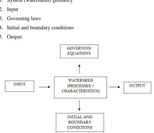
A model, as shown in Fig. 1.6 has five components:
1. System (watersheds) geometry 2. Input
3. Governing laws
4. Initial and boundary conditions 5. Output
1.1.2 Structure classification for black-box models
In connection with hydrological models of their structure rainfall-runoff transformation can be classified as:
- Hydraulic or detailed simulation models: based on experimental observations and analytical models attempt to simulate the individual hydrological processes that are then connected by appropriate mathematical relationships.
- Conceptual models: assimilate the real transformation of rainfall to bring in another, referred to a physical system, even different, but can provide a similar response. In this category, you can frame models with very different structures: one can identify both models is complex, similar to hydraulic models, and models such as linear parameters, simple structure, similar to that of synthetic models.
- Synthetic model (or empirical or black box): are not intended to represent the processes hydrological and physical phenomena involved in rainfall-runoff transformation or physically or mathematically. They see the system as a closed box (black box) on which there is no specific hypotheses. Modelling, therefore, end with the search for a mathematical operator that links between them, in the best possible way, and incoming out of the system, or the meteor influx with flow flowing out to the closing section river basin.
Furthermore the models can be described as deterministic or stochastic. A deterministic model is a physical-mathematical model that tries to predict numerically the evolution of the climate system in space-time, through the approximate solution (not analytical) of the system of mathematical equations that describe the physical laws (the classical mechanics and of thermodynamics) that govern the system atmosphere.
Once the initialization process is terminated the system of equations, that make up the deterministic model, evolves towards a unique solution. In this way we have achieved something unique number for each point in space and at every point in time future.
A stochastic model is a model consisting of a finite set of random variables that depend on a parameter "t", with which we generally mean time, and the values that the individual random variables have undertaken in the past, namely with respect to a statistical basis of departure.
The initialization of the random variables is done through the identification of the probability distribution that characterizes each variable, through statistical analysis of a database collected in the past, which represents the probability space of the values that the random variable can assume.
Once rebuilt, the probability distribution of individual random variables can be simulated via the stochastic model, the variation in time of the probability distribution of random variables, resulting in a new probability space of values for each random variable.
1.1.3 Space-scale based classification
This classification is extremely important from a practical point of view. The hydrological model is said concentrate when the volume control reference for the application of constitutive equations is extended to large spatial scales, typically entire river basin. In this case, the model has no spatial dimensions. The model is, instead, said spatially distributed if the volume control is extended to very small spatial scale, so that within it is plausible the assumption of homogeneity of hydrological processes. Typically, the watersheds with area of 100 km2 or less can be called small, those with area of 100 to 1000 km2 medium, and those with area of larger than 1000 km2 large.
1.1.4 Land-use based classification
Hydrological models divided into two major categories. We talk about patterns of generation of synthetic series when the aim of work is to reproduce artificial hydrological variables, or variables that do not occur in reality. An example are the models for estimating flood flow.
The simulation models of observable variable, however, are designed to reproduce the variables that have occurred or will occur in the real world, independently from the availability or otherwise of the corresponding observed value. For instance, forecasting models and reconstruction models of observed events.
1.1.5 Model-use based classification
Many hydrological models are designed to produce simulations that are carried out over short time periods. This approach is justified by the necessity, which occurs when applying rainfall-runoff models, to have extended simulations to a single flood event, because we do not consider the simulation in periods of lean and tender. In this case we say that the model works at scale event. We speak instead of a continuous simulation model over time if the model is designed to produce simulations of long time span.
Nowadays, continuous simulation models receive attention from the scientific community, because are gaining interest the problems of the management of water resources during low flows.
CHAPTER 2
MODEL CALIBRATION
The practice application of a hydrological model is divided into the following stages:
1. Operational problems identification; 2. Model identification;
3. Calibration procedure selection; 4. Calibration;
5. Model verification.
Operational problems identification is a very delicate phase for the operator that must clarify what is the purpose of applying the model, in all its facets. Availability of data and technical requirements should be analyzed with great precision.
Model identification is made on the basis of technical requirements, and also according to the models available in the literature, hydrologist chooses the most appropriate model but the superiority of one approach than another is influenced from the scope.
For the selection of the calibration procedure we can make similar considerations. The calibration can be performed by two different alternatives: the manual calibration and automatic calibration which will be discussed in the next paragraph. In general, the automatic calibration requires more time and more availability of observed data. The manual calibration instead requires great sensitivity of the engineer who must understand how to change the parameters for improving the model performance. The parameters, that most influence on the results of the simulation, will be subject to more study in the calibration phase.
Model verification is a very important step because it gives information about the real functioning of the model unlike the calibration. After testing the model, it is appropriate to repeat the calibration using the full range of available data, in order to maximize the consistency of the database used to estimate parameter values.
2.1 Introduction to model calibration
The hydrological models are characterized by the presence of parameters to be set by the user. Obviously, different values of parameters correspond to different responses of the model and thus parameters variability allows the model to interpret the different characteristics of different river basins.
The procedure for assigning parameter values, which must precede so any practical application, is called parameters (or models) calibration, model parameterization, parameters (or model) optimization.
Usually the calibration is carried out by searching the parameter values that maximize the reliability of the simulation made by the model.
For modelling the rainfall–runoff process, models, that have been developed, are based on conceptual representations of the physical processes of the water flow lumped over the entire catchment area (lumped conceptual type of models). Examples of this type of model are the Sacramento model (Burnash et al., 1995), the Tank model (Sugawara et al., 1995), the HBV model (Bergstrom et al., 1995), and the MIKE 11/NAM model (Nielsen and Hansen, 1973; Havnø et al.,1995).
All rainfall-runoff models are so a simplifications of the real-world systems under investigation. The model components are aggregated descriptions of real world hydrologic processes. One consequence of this is that the model parameters often do not represent directly measurable entities, but must be estimated using measurements of the system response through a process known as model calibration. In fact all rainfall-runoff models are to some degree lumped, so that their equations and parameters describe the processes as aggregated in space and time. As a consequence, the model parameters are typically not directly measurable, and have to be specified through an indirect process of parameter estimation, that is called calibration.
To calibrate a model, values of the model parameters are selected so that the model simulates the hydrological behaviour of the catchment as closely as possible.
2.2 Model parameters
Such models typically have two types of parameters: “physical” parameters and “process” parameters.
• Physical parameters: represent measurable properties of the watershed like the area of the watershed, the fraction of the watershed area that is impervious, and so on.
• Process parameters: represent watersheds properties that are not directly measurable like the depth of surface soil moisture storage, the effective lateral interflow rate, and so on.
Due to the fact that in the range of possible (or already observed) input data, different model parameters lead to a similar performance, the identification of a unique dataset is practically impossible (Beven and Freer, 2001).
2.3 Manual calibration
In manual calibration, a trial-and-error parameter adjustment is made. In this case, the goodness-of-fit of the calibrated model is basically based on a visual judgment by comparing the simulated and the observed hydrographs. For an experienced hydrologist it is possible to obtain a very good and hydrologically sound model using manual calibration.
However, since there is no generally accepted objective measure of comparison, and because of the subjective judgment involved, it is difficult to assess explicitly the confidence of the model simulations. Furthermore, manual calibration may be a very time consuming task, especially for an inexperienced hydrologist.
2.4 Automatic calibration
In automatic calibration, parameters are adjusted automatically according to a specified search scheme and numerical measures of the goodness-of-fit. As compared to manual calibration, automatic calibration is fast, and the confidence of the model simulations can be explicitly stated. The development of automatic calibration procedures has focused mainly on using a single overall objective
function (e.g. the root mean square error between the observed and simulated runoff) to measure the goodness-of-fit of the calibrated model.
For automatic calibration is therefore necessary to establish a criterion for automatically and quantitatively compare the goodness of the simulation. For doing this, it use an objective function which is then minimized (or maximized) using the algorithms. The need for an objective function makes the automatic calibration using the shell is mainly when there are observed values of the data to be simulated, which are automatically compared with the corresponding simulated values. In this case, the objective functions can also be used in case of manual calibration, if you want the comparison between observed and simulated values occur quantitatively.
2.4.1 Objective functions
An objective function is an equation that is used to compute a numerical measure of the difference between the model-simulated output and the observed (measured) watersheds output.
The aim is so to find those values of the model parameters that optimize the numerical value of the objective function.
The objective functions mostly used are:
1. Weighted Least Squares: it is one of the most common used objective function. The weights wt indicate the importance to be given to fitting a
particular hydrograph value
= ∑ ∙ − 2
[2.1]
where:
− = observed (measured) streamflow value at time t;
− = model simulated streamflow value at time t;
− = vector of model parameters;
− = weight at time t;
2. Daily root-mean square (DRMS): The daily root-mean square (DRMS)
computes the standard deviation of the model prediction error (difference between measured and simulated values). The smaller the DRMS value, the better the model performance (Gupta et al., 1999). Gupta et al. (1999) determined that DRMS increased with wetness of the year, indicating that the forecast error variance is larger for higher flows. According to Gupta et al. (1999), DRMS had limited ability to clearly indicate poor model performance. The function is:
= ∑ − 2
[2.2]
3. Nash-Sutcliffe measure (NS): used to assess the predictive power of
hydrological models. It is defined as:
= 1 − ∑# ! "
∑# $ " [2.3]
Where d is observed discharge, ot is modelled discharge and dt is
observed discharge at time t. Nash–Sutcliffe efficiencies can range from −∞ to 1. An efficiency of 1 (E = 1) corresponds to a perfect match of modelled discharge to the observed data. An efficiency of 0 (E = 0) indicates that the model predictions are as accurate as the mean of the observed data, whereas an efficiency less than zero (E < 0) occurs when the observed mean is a better predictor than the model or, in other words, when the residual variance (described by the numerator in the expression above), is larger than the data variance (described by the denominator).
Essentially, the closer the model efficiency is to 1, the more accurate the model is. It should be noted that Nash–Sutcliffe efficiencies can also be used to quantitatively describe the accuracy of model outputs other than discharge. This method can be used to describe the predictive accuracy of other models as long as there are observed data to compare the model results. (Nash, J. E. and J. V. Sutcliffe et al.1970).
4. Bias (mean daily error):
E θ ='∑' d)− o) θ
) [2.4]
In statistics, bias (or bias function) of an estimator is the difference between this estimator's expected value and the true value of the parameter being estimated. An estimator or decision rule with zero bias is called unbiased. Otherwise the estimator is said to be biased.
5. ABSERR (mean absolute error): is a quantity used to measure how
close forecasts or predictions are to the eventual outcomes. The mean absolute error is given by:
F θ ='∑ |d') )− o) θ | [2.5]
The mean absolute error is a common measure of forecast error in time series analysis, where the terms "mean absolute deviation" is sometimes used in confusion with the more standard definition of mean absolute deviation.
The mean absolute error is one of a number of ways of comparing forecasts with their eventual outcomes. Well-established alternatives are the mean absolute scaled error and the mean squared error.
Where a prediction model is to be fitted using a selected performance measure, in the sense that the least squares approach is related to the mean squared error, the equivalent for mean absolute error is least absolute deviations. (Hyndman, R. and Koehler A. et al.,2005).
6. ABSMAX (maximum absolute error):
F θ = max|d)− o) | [2.6]
2.5 Optimization methods
An optimization algorithm is a logical procedure that is used to search the response surface, constrained to the allowable ranges on the parameters, for the parameter values that optimize (maximize or minimize, as appropriate) the numerical value of the objective function. The procedure is typically implemented on a digital computer to enable a very rapid search. There are a lot of methods for automatic calibration but we will describe just two that we will see in the application with HBV model, Genetic Algorithm (GA) and Harmony Search (HS).
2.5.1 Genetic algorithm (GA)
A genetic algorithm (GA) is a search heuristic that mimics the process of natural evolution. This heuristic is routinely used to generate useful solutions to optimization and search problems. Genetic algorithms belong to the larger class of evolutionary algorithms (EA), which generate solutions to optimization problems using techniques inspired by natural evolution, such as inheritance, mutation, selection, and crossover (Eiben, A. E. et al, 1994).
With a genetic algorithm calibration algorithm, optimized parameter sets are found by an evolution of parameter sets using selection and recombination. An initial population of n parameter sets is generated randomly in the parameter space and “fitness” of each set was evaluated by the value of the objective function. From this population (generation) is generated by n times combining of two parameter sets. The two sets were chosen randomly but the chance of being picked is related to the fitness of the parameter set giving the highest probability to the set with the highest fitness. A new parameter set was generated from the two parent sets (set A and B) by applying one of the following four rules for each parameter randomly with certain probabilities, p:
• Value of set A
• Value of set B
• Random between the values of set A and set B
The fitness of each set in the new population is evaluated and the new generation replaced the old one. This evolution is repeated for a number of generations (Jan Seibert et al.2000).
2.5.2 Harmony Search (HS)
A new heuristic algorithm has been developed and named Harmony Search (HS). Harmony search (HS) is a phenomenon-mimicking algorithm (also known as metheuristic algorithm, soft computing algorithm or evolutionary algorithm) inspired by the improvisation process of musicians. In the HS algorithm, each musician (= decision variable) plays (= generates) a note (= a value) for finding a best harmony (= global optimum) all together.
The goal of the process is to reach a perfect state of harmony. The different steps of the HS algorithm are described below:
Step 1:
The 1st step is to specify the problem and initialize the parameter values. The optimization problem is defined as minimize (or maximize) f(x) such that Lxi < xi<Uxi, where f(x) is the objective function, x is a solution vector consisting of N decision variables (xi) and Lxi and Uxi are the lower and upper bounds of each
decision variable, respectively. The parameters of the HS algorithm i.e. the harmony memory size (HMS), or the number of solution vectors in the harmony memory; harmony memory considering rate (HMCR); pitch adjusting rate (PAR); distance bandwidth parameter (bw); and the number of improvisations (NI) or stopping criterion are also specified in this step.
Step 2:
The 2nd step is to initialize the Harmony Memory. The initial harmony memory is generated from a uniform distribution in the ranges [Lxi, Uxi], where 1
< i < N. This is done as follows:
012 = 03 1 + 5 × 07 1− 03 1 [2.7]
where j = 1,2,3....,HMS and 5~9 0,1 .
Step 3:
The third step is known as the “improvisation” step. Generating a new harmony is called “improvisation”. The New Harmony vector is generated using
the following rules: memory consideration, pitch adjustment, and random selection.
Step 4:
In this step the harmony memory is updated. The generated harmony vector replaces the worst harmony in the HM (harmony memory), only if its fitness (measured in terms of the objective function) is better than the worst harmony.
Step 5:
The stopping criterion (generally the number of iterations) is checked. If it is satisfied, computation is terminated. Otherwise, Steps 3 and 4 are repeated.
2.6 Calibration strategies
There are different calibration strategies to meet two objectives: good discharge simulations in terms of least mean square errors and the ability to reproduce one functional characteristic of the system and the autocorrelation function of the discharge, which quantifies the linear dependency of successive values over time.
2.6.1 Split sample-test
The available record should be split into two segments one of which should be used for calibration and the other for validation. If the available record is sufficiently long so that one half of it may suffice for adequate calibration, it should be split into two equal parts, each of them should be used in turn for calibration and validation, and results from both arrangements compared. The model should be judged acceptable only if the two results are similar and the errors in both validations are acceptable. If the available record is not long enough for a 50/50 splitting, it should be split in such a way that the calibration segment is long enough for a meaningful calibration, the remainder serving for validation. In such a case, the splitting should be done in two different ways, e.g. (a) the first 70% of the record for calibration and the last 30% for validation; (b) the last 70% for calibration and the first 30% for validation. The model should qualify only if validation results from both cases are acceptable and similar. If the available record cannot be meaningfully split, then only a model which has passed a higher level test should be used. (Klemeš, V. et al., 1986).
2.6.2 Proxy-basin test
This test should be required as a basic test for geographical transposability of a model, i.e transposability within a region, such as for instance, the European Alps, the prairie region of Canada and the USA, etc. If streamflow in an ungauged basin C is to be simulated, two gauged basins A and B within the region should be selected. The model should be calibrated on basin A and validated on basin B and vice versa. Only if the two validation results are acceptable and similar can the model command a basic level of credibility with regard to its ability to simulate the streamflow in basin C adequately.
This kind of test should also be required when an available streamflow record in basin C is to be extended and is not adequate for a split-sample test as described above. In other words, the inadequate record in basin C would not be used for model development and the extension would be treated as simulation in an ungauged basin (the record in C would be used only for additional validation, i.e. for comparison with a record simulated on the basis of calibrations in A and B).
Geographical transposability between regions I and II (e.g. the Inland Waters Directorate of Environment Canada has identified a need to develop models for simulating streamflow in ungauged basins of northern Ontario; such models would have to be developed on the basis of data from gauged basins in southern Ontario or Quebec which have different physical conditions). If streamflow needs to be simulated in an as yet unspecified ungauged basin C (or on a number of such basins) in region II the procedure should be as follows. First, the model is calibrated on the historic record of a gauged basin D in region I. Streamflow measurements are started on at least two different substitute basins, A and B, in region II and maintained for at least three years. Then the model is validated on these three-year records of both A and B and judged adequate for simulation in a basin C if errors in both validation runs, A and B, are acceptable and not significantly different. After longer records in A and B become available, these two basins can be used for model development and subjected to the simpler test for transposability within a region as described above, using A and B as proxy basins for C. Of course, the substitute basins A and B, would not be chosen randomly but would be selected so as to be
representative of the conditions in region II, and, as far as possible, with due consideration of future streamgauging needs (Klemeš, V. et al.1986).
2.6.3 Differential split-simple test
This test should be required whenever a model is to be used to simulate flows in a given gauged basin under conditions different from those corresponding to the available flow record. The test may have several variants depending on the specific nature of the change for which the flow is to be simulated.
For a simulation of the effect of a change in climate, the test should have the following form. Two periods with different values of the climate parameters of interest should be identified in the historic record, e.g. one with high average precipitation, the other with low. If the model is intended to simulate streamflow for a wet climate scenario then it should be calibrated on a dry segment of the historic record and validated on a wet segment. If it is intended to simulate flows for a dry climate scenario, the opposite should be done. In general, the model should demonstrate its ability to perform under the transition required: from drier to wetter conditions or the opposite.
If segments with significantly different climatic parameters cannot be identified in the given record, the model should be tested in a substitute basin in which the differential split-sample test can be done. This will always be the case when the effect of a change in land use, rather than in climate, is to be simulated. The requirement should be as follows: to find a gauged basin where a similar land-use change has taken place during the period covered by the historic record, to calibrate the model on a segment corresponding to the original land use and validate it on the segment corresponding to the changed land use.
Where the use of substitute basins is required for the testing, two substitute basins should be used, the model fitted to both and the results for the two validation runs compared. Only if the results are similar can the model be judged adequate. Note that in this case (two substitute basins) the differential split-sample test is done on each basin independently which is different from the proxy-basin test where a model is calibrated on one basin and validated on the other (Klemeš, V. et al, 1986).
2.6.4 Proxy-basin differential split-sample test
This test should be applied in cases where the model is supposed to be both geographically and climatically (or land-use-wise) transposable.
Such universal transposability is the ultimate goal of hydrological modelling, a goal which may not be attained in decades to come. However, models with this capability are in high demand (e.g. in Canada for assessing the climate-change impact in northern regions where most basins are not gauged) and hydrologists are being encouraged to develop them despite the fact that thus far even the much easier problem of simple geographical transposability within a region has not been satisfactorily solved. (Klemeš, V. et al, 1986).
CHAPTER 3
HBV MODEL - HYDROLOGINSKA BYRANS
VATTENBALANSAVDELNING
The HBV hydrology model, or Hydrologiska Byråns Vattenbalansavdelning model, is a computer simulation used to analyze river discharge and water pollution. Developed originally for use in Scandinavia, this hydrological transport model has also been applied in a large number of catchments on most continents.
The HBV model is a conceptual hydrological model capable of simulating outflow from a river catchment, given meteorological input data and set of parameters.
3.1 Introduction
The HBV model (Bergstrom et al., 1976; 1992) is a conceptual model that simulates daily discharge using daily rainfall and temperature, and monthly estimates of potential evaporation as input. The model consists of different routines representing snow by a degree-day method, soil water and evaporation, groundwater by three linear reservoir equations and channel routing by a triangular weighting function.
The first successful run with an early version of the HBV hydrological model was carried out in the spring of 1972 (Bergstrom et al., 1972) (Figure 3.1):
Figure 3.1: The first successful application of the HBV model (Sten Bergstrom et al., 1972).
After twenty years the HBV model has become a standard tool for runoff simulations in the Nordic countries, and the number of applications in other countries is growing. Some of applications abroad are carried out by the Swedish Meteorological and Hydrological Institute using a standard computer code.
Its successor, the PULSE model, is used for hydrochemical simulations and simulations in ungauged catchments.
Work with HBV model has been reported on numerous occasions and in a large number of scientific papers.
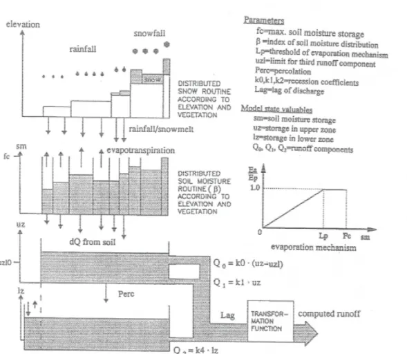
Figure 3.2: Scheme of the HBV model.
Symbols:
o Ssf is the snow storage in forest;
o Sso is the snow storage in open areas;
o Ssm is the soil moisture storage;
o Fc is the Max. soil moisture storage;
o Wp is the Min. soil moisture storage;
o Suz is the storage in upper zone;
o Luz is the limit for third runoff component;
o Slz is the storage in lower zone;
o Q0,Q1,Q2 are the runoff components;
Below is a summary of the input data required and output data produced by the HBV model. The model requires little geographical input data, only the size of the modeled catchments is needed.
Input data (daily values):
− Size of modeled catchments (km2);
− Lake surface height (m) – lake surface area (km2) curve;
− Precipitation (mm/d), one station, or weighted sum of several stations;
− Potential evaporation computed from one of the following:
o Pan evaporation (mm/d);
o Min and max temperature);
o Average temperature (°C), cloudiness (%);
o Average temperature (°C), short wave radiation (MJ/d), wind speed (m/s) and relative humidity (%);
− Average outflow (m3/s), one station;
Computed result (daily values):
− Average outflow (m3/s);
− Optionally model state variables (mm), evaporation (mm/d), corrected precipitation (mm), lake surface height (m) and lake area (km2);
3.2 The HBV model and its parameters
The HBV model is a rainfall-runoff model, which includes conceptual numerical descriptions of hydrological processes at the catchment scale. The general water balance can be described as:
Where:
o P is the precipitation;
o E is the evapotranspiration;
o Q is the runoff;
o SP is the snow pack;
o SM is the soil moisture;
o UZ is the upper groundwater zone ;
o LZ is the lower groundwater zone;
o lakes is the lake volume.
In different model versions HBV has been applied in more than 40 countries all over the world. It has been applied to countries with such different climatic conditions as for example Sweden, Zimbabwe, India and Colombia. The model has been applied for scales ranging from lysimeter plots (Lindström and Rodhe et al., 1992) to the entire Baltic Sea drainage basin (Bergström and Carlson et al., 1994; Graham et al., 1999). HBV can be used as a semi-distributed model by dividing the catchment into subbasins. Each subbasin is then divided into zones according to altitude, lake area and vegetation. The model is normally run on daily values of rainfall and air temperature, and daily or monthly estimates of potential evaporation. The model is used for flood forecasting in the Nordic countries, and many other purposes, such as spillway design floods simulation (Bergström et al., 1992), water resources evaluation (for example Jutman et al., 1992; Brandt et al., 1994), nutrient load estimates (Arheimer et al., 1998).
3.2.1 Parameters
In summary the model parameters of the HBV model are sixteen and the following definitions give basic information about the meaning of particular parameter, about their possible names and also some information about the interval from which it should be taken.
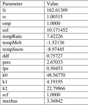
The parameters that we have to calibrate are:
Fc, field capacity – maximum amount of water the soil can hold [mm]; Rc (BETA), recharge coefficient – determines the contribution of
precipitation and melted snow to the soil and upper zone;
Emp (C), empirical parameter – used only when calculating daily PET from
monthly values of PET;
Uzl (luz), upper zone limit – determines the threshold in upper zone when
the discharge q0 occurs [mm];
tempRain – temperature threshold above which all precipitation is liquid
[°];
tempMelt (TT) – temperature threshold determining the melting of snow
cover [°];
tempSnow – temperature threshold below which all precipitation is solid
(snow) [°];
ddf (CMELT), degree day factor – determines the speed of snow melting
[mm];
perc , percolation – amount of water from upper to lower zone [mm];
lpe (LP), limit of potential evapotranspiration – used to estimate actual
evapotransipration [-];
k0,k1,k2, empirical parameters influencing the discharge from upper and lower zones;
croute- parameter affecting the distribution of flow into several days;
scf, CSF, snow correction factor – Snow accumulation is adjusted by a free
parameter; it should remain 1;
maxbas, number of days into which the flow from particular storages is
distributed.
The HBV model can best be classified as a semi-distributed conceptual model. It uses subbasins as primary hydrological units, and within these an area-elevation distribution and a crude classification of land use (forest, open, lakes) are made.
The HBV model consists of three main components:
1. Subroutines for snow accumulation and melt; 2. Subroutines for soil moisture accounting; 3. Response and river routing subroutines.
The model has a number of free parameters, values of which are found by calibration. There are also parameters describing the characteristics of the basin and its climate which remain untouched during model calibration. ( Bergstrom et al., 1992).
Input data are precipitation and, in areas with snow, air temperature. The soil moisture accounting procedure requires data on the potential evapotranspiration.
Areal averages of the climatological data are computed separately for each subbasin.
1. Snow submodel
The snow routine of the model controls snow accumulation and melt. The precipitation accumulates as snow when the air temperature drops below a threshold value (TT). Snow accumulation is adjusted by a free parameter, CSF,
the snowfall correction factor.
Melt starts with temperatures above the threshold, TT; according to a simple degree-day expression:
? AG = HIJ3K∙ G − GG [3.2.]
Where:
o MELT is a snowmelt (mm/day);
o CMELT is degree-day factor (mm/°C);
o TT is the threshold temperature (°C).
Thus the snow routine of the HBV model has primarily three free parameters that have to be estimated by calibration: TT, CSF and CMELT.
2. Soil moisture submodel
The soil moisture accounting routine computes an index of the wetness of the entire basin. It is controlled by three free parameters, FC, BETA and LP which will be discussed later.
Recently a modification of the evapotranspiration routine has been introduced in order to improve the model performance when the spring and summer is much colder or warmer than normal (Lindstrom and Bergstrom et al., 1992). This routine accounts for temperature anomalies by a correction which is based on mean daily air temperatures and long term averages according to this equation:
< L = 1 + H ∙ G − GI ∙ < I [3.3]
Where:
o PEA is a adjusted potential evapotranspiration;
o C is a empirical model parameter;
o T is the daily mean air temperature;
o TM is the monthly long term average temperature;
o PEM is the monthly long term average potential transpiration.
The three free parameters are:
o FC is a maximum soil moisture storage in the basin;
o BETA determines the relative contribution to runoff from a millimeter of rain or snowmelt at a given soil moisture deficit;
o LP controls the shape of the reduction curve for potential evaporation.
3. Runoff response submodel
The runoff response routine transforms excess water (∆Q) from the soil moisture routine, to discharge for each subbasin. The routine consist of two reservoirs with the following free parameters:
o K0, K1, K2 are three recession coefficients;
o UZL is the threshold;
Finally there is a filter for smoothing of the generated flow. This filter consists of a triangular weighting function with one free parameter, MAXBAS. It is a model parameter affecting the distribution of flow into several days.
3.3 Model calibration
The agreement between observed and computed runoff is evaluated by Nash and Sutcliffe efficiency criterion (Nash and Sutcliffe et al., 1970) which is commonly used in hydrological modeling:
M
N=
∑ P$Q PQ " ∑ P R PQ "∑ P$Q PQ " [3.4]
Where:
o Q0 is a observed runoff
o =$Sis the mean of observed runoff
o Qc is the computed runoff
A perfect fit would give a value of R2 = 1 , but in practice the value above 0.8 means good fit and measured hydrographs (IHMS, 1999).
CHAPTER 4
STUDY CATCHMENT: THE HRON RIVER
BASIN
One catchment was used in this study, the Hron river basin, located in Slovakia. The Hron River is a left-side tributary of the Danube River; its basin is located in Central Slovakia. The catchment is feather-shaped, located along the long main river with numerous shorter tributaries. It covers an area of 5465 km2; its upper and middle parts are situated in the area of Inner Carpathian Mountains, while the lower part of the basin belongs to the Danubian Lowlands. The spring of the Hron River is at an altitude of 934 m a.s.l. near the village of Telgárt and it flows into the Danube near Štúrovo at an altitude of at 103 m a.s.l. The total length of the Hron River is 284 km. The mean slope of the river varies from about 7.6 ‰ in the upper part to 0.9 ‰ in the lowlands. The Hron River drains 11.2 % of Slovakia. After the Váh and Bodrog catchments, the Hron is the third largest river in Slovakia. The most important tributaries in the upper part of the basin are Hronec, Čierny Hron and Rohožná from the left, Bystrá, Vajskovský and Jasenský potok from the right side. In the middle part of the basin the Slatina is the largest tributary; other important tributaries are Bystrica, Kremnický and Žarnovický potok.
With regards to the availability of hydro-meteorological data and also according to the character of the hydrologic processes in the catchment the alluvial part of the river has not sufficient data suitable for hydrologic modelling (short series and less a dense network). However, due to its lowland character and very low specific discharge (mostly less than 1.5 l s-1 km-2), modelling approaches have to be applied which better account for the physically based description of processes in the unsaturated zone than conceptual rainfall-runoff models. Therefore the discharge gauging station Banská Bystrica was selected as the closing cross section for this study (the term “Hron River basin” refers mainly to the Hron catchment to Banská Bystrica hereafter). This upper Hron River basin up to the Banská Bystrica gauging station has an area of 1766 km2, the minimum elevation of the basin is 340 m a.s.l.; the maximum elevation is
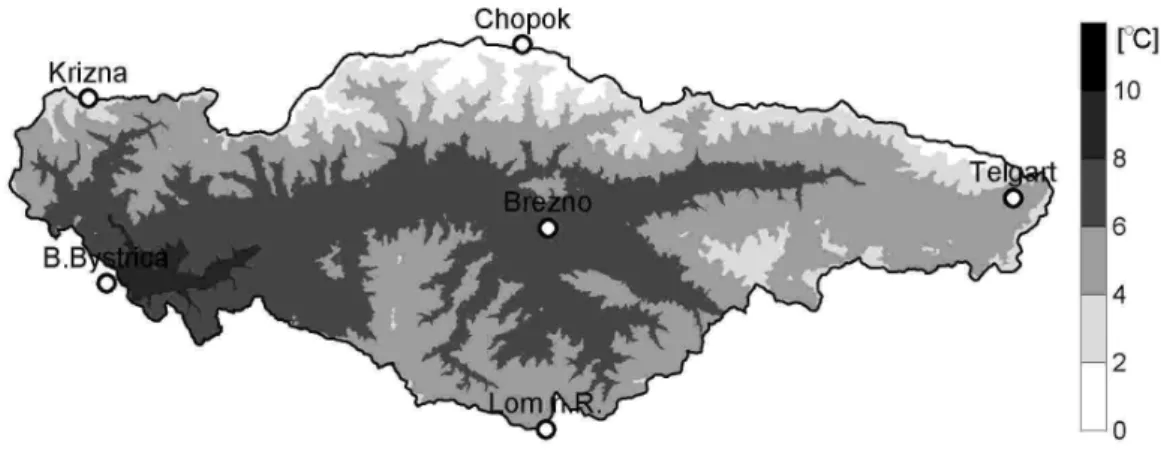
2004 m a.s.l.; and the mean elevation is 850 m a.s.l. The location of the basin in Slovakia is shown in Figure 4.1:
Figure 4.1: Location of the Hron River in Slovakia.
The climatic conditions of the Hron River basin correspond to the European-continental climatic region of the mild zone, with oceanic air masses transforming into continental ones. The annual precipitation in the basin varies from 570 to 700 mm year-1 in the lowlands to about 700 - 1400 mm year-1 in the valleys and upper mountainous areas. The overall average is approximately 800 mm year-1. Evaporation amounts to approximately 300 to 600 mm year-1.
Three regional subdivisions of the catchment can be made according to relief and elevation: the warm region (lowlands), which is spreading out in the Danube lowland, the Žiar and Zvolen Valleys, the mild-warm region (valleys), which covers the mountain slopes up to 800 m a.s.l., and the whole Upper Hron Valley. The third, the cold region (mountainous slopes), is located above 800 m a.s.l. in all mountains surrounding the upper part of the basin. The basic climatic characteristics of these sub-regions are given in Table 4.1.
The Hron River has a snow-rain combined runoff regime type. The precipitation in the upper part of the Hron basin reaches 1600 mm, while in lower flat areas it is only 600 mm. The runoff represents in the upper part up to 60 % of the precipitation, while in the flatlands only 10 %, the mean value for the whole basin being 37 %. The long-term mean annual discharge for the Hron in Brezno is 8.12 m3 s-1, in Banská Bystrica 28.0 m3 s-1, and at the confluence with the Danube it increases to 55.2 m3 s-1 (Table 4.2).
The specific runoff in the Hron River basin varies between 1.6 in the lowlands to 28 l s-1 km-2 in the mountains. The richest tributaries are Bystrianka, Jaseniansky potok, Vajskovský potok and Bystrica, where these values reach 22 - 25 l s-1 km
-2
. In the flatland areas the specific yield is only 1.5 l s-1 km-2. The mean values for the whole basin is 10.1 l s-1 km-2 which is 20 % more than that for the whole territory of Slovakia.
The flood generation problem in the basin is complex. In the alpine high mountain regions floods from snowmelt, mixed events and flash floods represent a threat to local villages build in narrow valleys all over the year. Due to runoff concentration snowmelt floods and floods of cyclonic origin represent danger to major cities and industrial areas with heavy and chemical industry, electric and atomic power plants in the middle of the catchments.
Table 4.1: Climatic characteristics of the Hron Basin (based on data provided by the Slovak Hydrometeorological Institute).
Climatic characteristics Lowlands Valleys Mountainous slopes
Mean temperature in January [°C] -1.5 to -2.5 -2.5 to -6.5 -2.5 to-8.0
Mean temperature in July [°C] 20.3 to 19.5 19.5 to 14.5 19.5 to 9.5
Days with temperature above 0 [°C] 320 - 300 300 - 245 300 – 195
Number of summer days 75 - 60 60 - 20 60 - 0
Number of ice days 25 - 35 35 - 50 35 - 75
Days with precipitation above 1 mm 85 - 100 100 - 120 100 - 150
Annual precipitation [mm] 580 - 700 700 - 900 700 - 1400
Precipitation in the warm season [mm] 330 - 400 400 - 500 400 - 750
Precipitation in the cold season [mm] 250 - 300 300 - 400 300 - 650
Number of days with snow cover 35 - 50 50 - 100 50 - 220
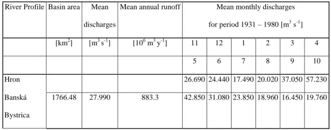
Table 4.2: Discharge characteristics in selected profiles in the Hron basin (based on data provided by the Slovak Hydrometeorological Institute).
River Profile Basin area Mean discharges
Mean annual runoff Mean monthly discharges
for period 1931 – 1980 [m3 s-1] [km2] [m3 s-1] [106 m3 y-1] 11 12 1 2 3 4 5 6 7 8 9 10 Hron 26.690 24.440 17.490 20.020 37.050 57.230 Banská Bystrica 1766.48 27.990 883.3 42.850 31.080 23.850 18.960 16.450 19.760
Table 4.3: Water balance characteristics of the Hron River and its tributaries in the period of 1931 – 1980 (based on data provided by the Slovak Hydrometeorological Institute).
Hron River mouth Bystrianka Vajskovský potok
Jaseniansky potok Bystrica
Precipitation [mm] 869 1414 1466 1407 1194 Runoff [mm] 319 755 820 704 722 Losses [mm] 550 659 646 703 472 Runoff coefficient 0.37 0.53 0.56 0.50 0.60 Specific runoff [l s-1 km-2] 10.10 23.92 25.98 22.31 22.89
Extensive studies conducted by the Slovak Hydrometeorological Institute have shown that hydrological time series from the periods 1931 to 1960 and from 1931 to 1980 can be considered stationary. When comparing statistical data from the period 1961 – 2000 with the long term behaviour of the catchments as described by data from the period 1931 – 1980, occasionally a slight decrease in runoff can be shown. The decrease in runoff is approximately the same for the Hron as for the whole country (about 10 %), precipitation decrease is less significant (about 1 to 4 %). In consequence there was a slight increase in evapotranspiration in the water balance. As for long-term mean monthly discharges for the same two periods, both increase an decrease can be detected in
the Hron river basin; the mean monthly discharges do not necessarily decrease in all months in all catchments. An increasing tendency can be detected in some catchments in the spring and early winter.
4.1 Description of the pilot basins
For the estimation of climate change impact on the annual, monthly and flood runoff one gauging station was selected in this study: Banská Bystrica. Table 4.4 contains the characteristics of the upper Hron basin and of the nested subcatchment: the mean basin values of air temperature, precipitation and runoff represent the mean annual averages from the period 1981 – 1990.
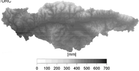
Table 4.5 shows the basin averages of long-term mean annual potential evapotranspiration (EP) and long-term mean annual actual evapotranspiration (ET) period 1981 – 1990 computed by the Turc model, which is used in this study. The spatial estimates of the long-term mean annual air temperature (1981 – 1990) from the six climatic stations, where the daily measurements of air temperature, air humidity, sunshine duration, vapour pressure and wind speed were carried out, are shown in Figure 4.2. Figure 4.3 shows the map of spatial estimates of the long-term mean annual precipitation (1981 – 1990) and precipitation stations (as points) used in interpolation of the map. The grid maps of the long-term mean annual potential and actual evapotranspiration (1981 – 1990) as estimated by the Turc empirical model from the precipitation, air temperature and runoff maps are shown in Figures 4.4 and 4.5.
Table 4.4: Basic characteristics of Banská Bystrica sub-basins from the period 1981 – 1990.