ALMA MATER STUDIORUM - UNIVERSITÀ DI BOLOGNA
SCUOLA DI INGEGNERIA E ARCHITETTURA
DIPARTIMENTO DI INFORMATICA – SCIENZA E INGEGNERIA CORSO DI LAUREA MAGISTRALE IN INGEGNERIA INFORMATICA
TESI DI LAUREA
in
COMPUTER VISION AND IMAGE PROCESSING
3D Object Detection from Point Clouds with dense pose voters
Candidato Relatore:
Mattia Fucili Chiar.mo Prof. Luigi Di Stefano
Correlatore/correlatori
Dott. Ing. Federico Tombari1
PhD Fabian Manhardt1
1Technische Universität München
Anno Accademico 2017/18 Sessione III
Summary
Introduction 10 Thesis outline . . . 11 1 Theory 12 1.1 Computer Vision . . . 12 1.1.1 Pinhole camera . . . 12 1.2 Machine Learning . . . 131.3 Supervised Learning algorithms . . . 14
1.3.1 Classification . . . 15
1.3.2 Regression . . . 16
1.3.3 Semi-supervised Learning algorithms . . . 17
1.4 Unsupervised Learning algorithms . . . 18
1.4.1 Clustering . . . 18
1.4.2 Association Rules . . . 18
1.5 Focus on Neural Networks . . . 19
1.5.1 Compute the error . . . 20
1.5.2 Gradient descent . . . 21
1.6 Convolutional Neural Networks . . . 24
1.6.1 Convolutional layer . . . 25
1.6.2 Activation function . . . 27
1.6.3 Pooling layer . . . 28
1.6.4 Fully Connected layer . . . 28
1.6.5 Convolutional Neural Network . . . 29
2 Related Work 31 2.1 2D object detection . . . 31
2.2 3D object detection . . . 31
2.2.1 Hand crafted features proposal generation . . . 31
2.2.2 Monocular-based proposal generation . . . 32
2.2.3 3D region proposal networks . . . 32
2.2.4 Region proposal from LIDAR and images . . . 33
2.2.5 RPN free architectures . . . 33
3 Data Analysis 35
3.1 Datasets for autonomous driving . . . 35
3.2 The KITTI dataset . . . 36
3.3 Data preparation . . . 39
3.3.1 Class labeling of Lidar points . . . 40
3.3.2 Computing the centroid . . . 42
3.3.3 Annotation of 3D Bounding Box . . . 43
4 Project and Solution 46 4.1 Classification . . . 46
4.2 Centroid vectors regression . . . 49
4.3 Bounding boxes regression . . . 52
4.3.1 Robust corner detection . . . 55
4.3.2 Clustering for real application of the model . . . 56
4.3.3 Other improvements to our model . . . 56
5 Experiments 58 5.1 Data Augmentation . . . 58
5.2 Network configuration . . . 58
5.3 Results . . . 58
5.3.1 Classification results . . . 58
5.3.2 Bounding box results . . . 60
5.3.3 Test on the ”road” . . . 61
5.3.4 Other results . . . 64 5.3.5 Numerical results . . . 67 Conclusion 73 Greetings 75 List of figures 78 List of tables 79 References 85
Abstract
Object detection has been always a challenging task in Computer Vision. It finds application in many fields, mostly in industry, such as finding the objects to be grabbed by a robot. In the last decades, such tasks have found new ways to be addressed thanks to the reemergence of Neural Networks, es-pecially Convolutional Neural Networks. This kind of networks has reached impressive results in many applications for object detection and image clas-sification. The trend now is to use such networks also in the automotive industry to make the dream of cars that drive alone become a reality. There are many prominent works on car recognition from 2D images. In this thesis we present our Convolutional Neural Network architecture for recog-nizing cars and estimating their positions in space, using only lidar inputs. We store the information of the bounding box around the car at point level ensuring us good prediction also in occluded situations. Tests are performed on the most used data set for car and pedestrian detection in autonomous driving applications.
Prefazione
Il riconoscimento di oggetti `e sempre stato un compito sfidante per la Computer Vision. Trova applicazione in molti campi, principalmente nell’industria, come ad esempio per permettere ad un robot di trovare gli oggetti da af- ferrare. Negli ultimi decenni tali compiti hanno trovato nuovi modi di es- sere raggiunti grazie alla riscoperta delle Reti Neurali, in particolare le Reti Neurali Convoluzionali. Questo tipo di reti ha raggiunto ottimi risultati in molte applicazioni per il riconoscimento e la classificazione degli oggetti. La tendenza, ora, `e quella di utilizzare tali reti anche nell’industria automo- bilistica per cercare di rendere reale il sogno delle automobili che guidano da sole. Ci sono molti lavori importanti sul riconoscimento delle auto dalle immagini. In questa tesi presentiamo la nostra architettura di Rete Neurale Convoluzionale per il riconoscimento di automobili e la loro posizione nello spazio, utilizzando solo input lidar. Salvando le informazioni riguardanti le bounding box attorno all’auto a livello del punto ci assicura una buona pre- visione anche in situazioni in cui le automobili sono occluse. I test vengono eseguiti sul dataset pi`u utilizzato per il riconoscimento di automobili e pedoni nelle applicazioni di guida autonoma.
Introduction
Autonomous driving has been one of the most challenging research in the past decade. Experiments in self-driving cars have been conducted since the 1920s. The first promising trials took place in the 1950s with cars guided by lights installed on the edge of the road and from that time the work still proceeds. The first truly self-guided car appeared in the 1980s with the ALV project[1]. So far, the obstacles are identified as clusters in the street but the approach is changing. To address this task, now, the most used tools are the Convolutional Neural Networks (CNNs) which, in the last decade, have achieved impressive results for object recognition in lots of application with images and for this reason they have been used also for autonomous driving purposes. Major car companies started to invest and test self-driving cars from the 2010s. Computer vision is a core part of these systems because it allows vehicles to know the environments, to see the obstacles and navigate the world.
Self-driving cars must be able to recognize 3D objects in the space in order to navigate. To do that they must be equipped with cameras and/or 3D sen-sors, like LIDAR[2]. There are many works implemented using RGB images, LIDAR and both. Some promising examples are VoxelNet[3] which works only with LIDAR data organized in voxel. AVOD[4] which uses both inputs to extract features and ROI-10D[5] which uses an image approach together with depth maps to detect cars.
In our work we have chosen to use point clouds because they carry more in-formation about the shapes of the obstacles, the spatial distributions and the depth, instead of simple 2D images which may carry problems of ambiguity. For example big car far away can be as small as car very close. Point clouds are captured using 3D scanners which fire pulsed laser light to a target and measure the reflected pulses with a sensor. This allows making the 3D model representation of the target. Point clouds found place in many fields; they are mostly used in the industrial world as 3D CAD models for manufactured parts, rendering and animation in film and games and even in medical appli-cations. In recent years they have found usage also in autonomous driving applications together with deep learning. Due to the high number of points inside a point cloud, work with them can be computationally very expensive. In the next chapters we show how to build a CNN model to solve two prob-lems: estimate the 3D bounding boxes surrounding the cars, pedestrians and vans and estimate their orientation along the street.
Thesis outline
First, we give a brief introduction to the thesis. In the first Chapter, we introduce the reader to computer vision and machine learning, its application in the real world and a dedicated sub-chapter focused on convolutional neural networks.
In Chapter 2 we explore the related works on object detection, especially in the autonomous driving context.
In the third Chapter we analyze a bunch of autonomous driving datasets, giving pros and cons compared to our goal. We then introduce the reader to the dataset we use, motivating the choice, and explain how it is structured using both images and tables. Lastly, we talk about how we have modified the data in order to feed them into our model.
Chapter 4 describes the convolutional model we present to solve the problem and explains all the design choices we have taken to get the final result. The experiments we did are presented and discussed in Chapter 5.
Finally, we conclude with the Conclusion Chapter in which we also give future work discussion.
1
Theory
In this chapter we introduce the reader to the concept of Machine Learning (ML) and its applications. In the beginning, we give some general infor-mation regarding what is ML, the di↵erent types of algorithms and their applications. In the last subchapter, we dive into the Convolutional Neural Network, which is the branch of ML we choose to accomplish the thesis.
1.1
Computer Vision
Computer vision is a scientific field, inspired by the human vision system, which deals with acquire, process, analyze and extract information from im-ages. A naive model to capture images is the pinhole camera model.
1.1.1 Pinhole camera
The simplest and well known camera model in computer vision is the pinhole model. It is an imaging device which gathers the light rays reflected by 3D objects to create a 2D representation of the scene. It can also be used to extract 3D information from 2D images. The image is captured by drawing the rays from scene points through the hole to the image plane.
Figure 1: Pinhole camera
The image formation process is known as perspective projection. The model is described with a center point C, the focal length f from C to the image
plane and c the intersection point between optical axis and image plane, called piercing point.
Figure 2: Pinhole camera model
Mathematically the model for the image formation process is described as 2 4uu 1 3 5 = 2 4f0x f0y ccxy 00 0 0 1 0 3 5 ⇤ 2 6 6 4 x y z 1 3 7 7 5
1.2
Machine Learning
Machine Learning is a topic which is getting more and more famous nowa-days. Its fields of application are increasing everyday. Firstly hypothesized in 1950 by Alan Turing who proposes a learning machine that could learn and become artificially intelligent[6]. Since that time a lot of new discoveries comes up; the first Neural Network machine in 1951, K-Nearest Neighbour algorithm in 1967, Recurrent Neural Network in 1982 and many more. To better understand all of this we give some theory explanations.
First of all, what does it mean Machine Learning? Machine Learning is a sci-ence who study algorithms and mathematical models to allow the computer
learning. In particular using a specific sample data, known as training data, the computer learns a mathematical model, which can be used to predict out-put without being programmed to do that. ML, as said before, find usages in di↵erent fields, such as email filtering, speech recognition, computer vision, data analysis, fraud detection, even auto-tag in Facebook and countless other examples. Given a training dataset the computer progressively tries to find a function to map the input to output labels.
Depending on whether we have output labels or not, every ML algorithm could be grouped into two main categories: Supervised Learning algorithms and Unsupervised Learning algorithms.
1.3
Supervised Learning algorithms
In this class belong all the algorithms which in the training phase try to find a map function between the input and the output based on specific pairs of values called training dataset.
Given a set of pairs input-output{(x1, y1), (x2, y2), ...(xn, yn)} the supervised
learning algorithm tries to find a function such that Y = f (X), with X as input space and Y as output space. The way an algorithm learns is modelled as adjustments in the mathematical model based on the output error of the model’s prediction.
There are several algorithms for Supervised Learning, few examples are: • Naive Bayes Classifier
This classifier is based on the Bayes’ Theorem and on the assumption of independence between the predictions.
• Support Vector Machines
Also abbreviated as SVM, this method seeks a hyperplane to separate the samples into two classes. One goal is to maximize the distance between the closest sample of the classes.
• Decision Trees
As the name suggests the structure of this method recall the shape of a tree. The dataset is split into parts based on an attribute value test inside the decision nodes and the classification are stored in the leaf nodes.
• Random Forest
at training time and to produce an output computing the mode of the classes for all the trees.
• K-Nearest Neighbour
This algorithm takes a bunch of labelled samples and uses them to learn how to label unseen examples. The K in the name of the method means the number of neighbours the algorithm checks to assign the label.
• Neural Networks
A Neural Network consists of layers of neurons that takes an input vector and outputs another. A neuron is the simplest brick of this method and is described as
y = wx + b (1)
Typically to a neuron is applied a non-linear function which is needed to be able to stack multiple layers. The Network is built connecting together several neurons where the output of one neuron is the input of another.
These problems can be further grouped in classification problems and regres-sion problems (Fig.3).
Figure 3: Machine Learning structure
1.3.1 Classification
A Supervised Learning algorithm is called a classification problem when the output variable to be predicted is a discrete value. For example, a standard
classification problem is to determine if the email is spam or not spam. In a nutshell a classification problem tries to predict discrete labels, class or categories. If the number of discrete values in output is two, usually the problem is called a binary classification problem; if there are more, then the problem is a multi-class classification problem.
The prediction could be also a continuous value as a probability to belong to a class or to another. Then this value, usually, is converted into the class with the highest probability. Using the example of the emails, one email can have the probability of being a spam email of 30% and 70% to not be spam. In this case, the email is labelled as not spam, since the highest probability suggests it.
Figure 4: Email example
To estimate the goodness classification skills of these algorithms there are several indices, but the most common is the accuracy index.
It consists on computing the percentage of correctly classified over all the predictions:
accuracy = correctprediction
totalprediction ⇤ 100 (2)
1.3.2 Regression
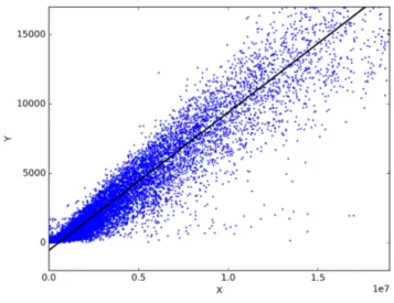
Regression tasks are very similar to classification tasks except for the type of output prediction, which is continuous. This means that with these kinds of methods we aim to predict: amount, price, weights, etc. A pretty standard example of this category is to estimate the price of a house in a specific region of the world.
The simplest method used to solve this problem is linear regression. This method is based on finding the best linear function that maps the input to the output. In the case of one variable the equation is the following:
y = wx + b (3)
with w and b called intercept and slope, which are the parameter to learn. The Fig.5 represents the graphical representation of the problem.
Figure 5: House price example
To estimate the goodness of the regressor, usually is used the Root Mean Squared Error (RMSE) index.
It consists of computing the square root of the average error between the predictions and the labels:
RM SE = v u u tXN n=1 (pi li)2 N (4)
with pi being the predicted value and li denoting the label.
1.3.3 Semi-supervised Learning algorithms
This is a particular class that during the training phase uses both labelled and unlabelled samples. Typically, this approach is used when there are more
unlabeled sample than labelled ones. These algorithms use the labelled data to produce labels for the other samples, reducing consistently the time and the cost needed to produce an entire labelled dataset. Moreover, since some samples have the label the whole process gains an improvement in learning accuracy with respect to the Unsupervised Learning.
1.4
Unsupervised Learning algorithms
An Unsupervised Learning algorithm is characterized by a training dataset without labels. These approaches are used to find common information in the input data, to group them and use the model obtained to label more unseen samples. Since there aren’t any labels to compute the error, is difficult to define a good model.
The most common algorithms to work with are: • K-Means[7]
• Neural Networks
• Principal Component Analysis (PCA)[8]
These methods can be further grouped in clustering problems and association rules problems.
1.4.1 Clustering
This approach is used when we want to discover hidden grouping in the input data. An example could be grouping costumer by a purchasing behaviour. There are many algorithms such as K-Means[7] which is a common algo-rithm used to tackle this kind of problems. Other well known algoalgo-rithms are Mean-Shift[9], DBSCAN[10] and agglomerative hierarchical clustering (HCA)[11][12].
1.4.2 Association Rules
This method is used to discover rules that describe your data in order to help the user to make decisions. Using the above example of the customers, an association rules algorithm is useful to find which products the customer buy together with other products. Apriori algorithm implements this behaviour.
1.5
Focus on Neural Networks
Artificial Neural Networks (ANN) are one of the recent tool used in Machine Learning. They are computing systems inspired by the human brain, as sug-gested the word ”neural”. A neural network is a collection of a units called neurons organized in layers connected together similar as synapses. Each neuron receives a signal modelled as input real value, processes it and then outputs it into the other neurons of the next layer, till the very last which outputs the prediction. This framework is very useful when the task requires to find a pattern which is very complex to discover by a human.
Neural networks have been introduced in the ’50 as perceptrons realized in hardware from Rosenblatt[13]. In the last decades, they have seen their widespread use thanks to the growth in computational power of the comput-ers.
The structure of a simple neural network is shown in Fig.6.
Figure 6: Neural Network sample structure
Each neuron and connection have its own weight which are adjusted as the learning process proceeds. They increase or decrease depending on the gra-dients from the error in the output. This process of updating the weights is called back-propagation. Moreover, every neuron also has a function which applies to the output, except for the final layer. This function is called the activation function. The activation functions are used to stack layers other-wise we can not model deep networks.
A neuron mathematically is modelled as follows: y = f (
N
X
with y as the output value, f the activation function and wixi respectively
the weights and the inputs. Typically a neural network with one hidden layer is used to model linear problems, on the contrary network with more than two hidden layers are used to model non-linear problems. Some common, non-linear, activation function are Sigmoid, ReLU, TanH and Leaky ReLU. The most used is the (Rectified Linear Units) ReLU function because it has a first order derivative which is a desirable property for enabling gradient-based optimization methods. It is defined as follows
y = max(0, x) (6)
In Fig.7 are shown three activation functions.
Figure 7: Activation functions
The basic neural network possible is the feed-forward neural network, which is a one-way network where the input passes through all the hidden layers to the output layer, without any weights updates.
1.5.1 Compute the error
Before dive into the weights updates we define the most used error functions and how to compute them. The loss is defined as y = L(y, y). There are many di↵erent ways to compute it and they depend on the type of the value, but the most known are:
• Mean Squared Error (MSE)
Known also as L2 Loss Function, it’s the most used for regression tasks and consists on computing the mean over the squared error di↵erence between the output and the ground-truth. L = N1 PNi=1(yi yi)2
• Mean Absolute Error
It’s also called L1 Loss Function and it’s defined as follows: L = 1
N
PN
i=1|yi yi|
• Log Loss
The Cross Entropy is used for classification tasks and is computed as: L = PNi=1yilog(yi)
1.5.2 Gradient descent
Since we want to minimize the error in the output of our network we need an optimization algorithm able to find the local minimum of a function. This concept is implemented following the gradient descent algorithm.
To explain this approach we must remind that if a multi-variable function F(x) is definite and di↵erentiable in a neighbourhood of a point p then, F(x) decreases very fast if we move from p to the direction of the negative gradient rF(p). This could be applied in the neural network to update the weights trying to find optimal values. A single step of an update can be written as
W+1 = W ↵rf(x) (7)
with W+1 as the next step, W the current step and ↵ the learning rate. The
learning rate plays a big role in this formula because it determines how big is the update. It is difficult to set a good one, because if the learning rate is too high the step is big and may happen that it will not reach the minimum but it bounces back and forth causing the so-called ”overshooting”. If the learning rate is set too small it will take a very long time to reach the solu-tion.
To update the weights we must compute the partial derivative @f /@w for any weight in the network. It’s clear that if the network is big this ap-proach in unfeasible. To overcome this problem has been introduced the back-propagation [14]. This method allows computing the derivatives from the output to the input passing through all the intermediate weights using the chain rule, which states:
@y @x = @y @u @u @x (8)
A good explanation example is shown in Fig.9.
Figure 9: Back-propagation example
The problem of the Gradient Descent is that it must see the entire dataset before performing a weights update step, making it very slow and even un-feasible with huge datasets.
To address this problem have been introduced many other methods based on it. Here a list of the most known:
• Stochastic Gradient Descent (SGD)
It updates the weights after each batch, making this process faster. Due to this high update frequency and fluctuation of the loss function, it struggles to converge.
• Momentum [15]
This techniques was invented to speed up the convergence of the SGD forcing the step updates in the right direction and softens the oscilla-tions.
v+1 = ⇢v + rf(x) (10)
W+1 = W ↵v+1 (11)
• Nesterov Momentum
It fixes a problem in the Momentum SGD which could lead to miss the minimum. Near the minimum the Momentum has a high value and since it does not know when to slow down the speed it may miss that point.
v+1 = ⇢v + rf(x + ⇢v) (12)
W+1 = W ↵v+1 (13)
• AdaGrad [16]
It uses di↵erent learning rate based on the past gradients. It makes big updates for infrequent parameters and small updates for frequent parameters.
g+1 = g + (rf(x))2 (14)
W+1 = W ↵p rf(x)
g+1+ 1e 7
(15) • Adaptive Moment Estimation (Adam) [17]
It compute adaptive learning rates and an exponential decay average of the past moments
There are many other types of Neural Networks, such as: • Convolutional Neural Networks (CNN)[18]
Particularly suitable to deal with images and for this reason are widely used in Computer Vision tasks.
• Recurrent Neural Networks (RNN)
RNN are a family of Neural Network for processing sequential data. Their hidden layers are characterized by having their output signal in input to the next layer and also in the input of themselves. This partic-ular configuration grants them the power to make a decision influenced by the past iterations. Are used for example in text analysis. particular types of RNN are the Long Short-Term Memory Networks (LSMT)[19] and GRU[20].
• Generative Adversarial Networks (GAN)[21]
Is a network composed of two networks, one used to generate samples and one to evaluate them. GANs are applied to align distribution by having a generator G. The generator generates a sample and a discrim-inator D tells if this sample comes from the corresponding distribution or not. The network is trained doing cycles of generate and test. In the next subsection, we will give more information about CNNs which is the tool used to carry out the thesis.
1.6
Convolutional Neural Networks
As aforementioned, CNNs are a category of the Neural Networks that are a powerful tool to address image recognition and classification tasks. They are largely used in face recognition (like in the smart-phones), robotic vision and self-driving cars.
The first artificial neural network was proposed by Kunihiko Fukushima in 1980s for handwritten character recognition [22]. It has inspired the first work on CNNs which was the pioneering Yann LeCunn network named LeNet5[18], used firstly to recognize characters.
The basic units to build a CNN are the following: • Convolutional layer
• Activation function • Pooling layer
First, we define what is the standard input of a CNN. As we said it works with images, and the simplest image in the input is a grey-scale image. Let the input image has a shape of W ⇤ H, so the input of our network is a grid of W xH numbers which span from 0 to 255.
Figure 10: Grey-scale image example
1.6.1 Convolutional layer
This layer is the most important, because it has the job to extract the fea-tures. It owes its name to the Convolution operator. This operator can extract features working with a small square portion of the image preserving the spatial information.
Suppose we have a grey-scale image and the top left corner portion of it.
Then we define a matrix called ”Kernel” which for example is the one of the Fig.12 below.
Figure 12: Kernel matrix
The convolution consists of summing up all the products between the input image and the kernel, applied in all the pixels. The Fig.13 gives an intuition of a step of the whole process.
Figure 13: Convolution example
An important parameter that we must define is the stride, this number in-dicates the number of pixel we want to skip when we slide our kernel on the image. Every time we apply a convolution process in a image, we get a a feature map with the size of
Loutput =
Linput Ksize+ 2P
stride + 1 (16)
with Loutput as the output size, Linput as the input size, Ksize as the size of
the kernel and P padding size.
stride 1 we end up with an image of size 6x6.
When the kernel is applied in the border of the image some pixels of the kernel don’t have the corresponding pixels of the image. In this case, the image is padded with zeros in order to not change the result of the sum. 1.6.2 Activation function
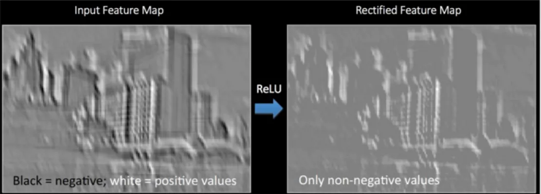
As we discussed before there are many non-linear activation functions that could be applied. The most used is ReLU.
If we do not add an activation function to our Network it can only model a linear function. This could be considered good because a linear function is a polynomial of one degree, but it lacks the power to learn complex functions, which is what we are looking for.
Just a reminder of the formula of the ReLU function
y = max(0, x) (17)
A good visualization of its application to an image is shown in Fig.14.
1.6.3 Pooling layer
Pooling layers are used to group features and usually to reduce the dimension of the space feature. Reducing the dimensions the number of parameters of the network is reduced and so the computational cost. The pooling layer can be of di↵erent types:
• max-pooling • sum-pooling • average-pooling
All of them consist in a window of a fixed size (for example 2x2) which is slide over the image and inside of it is applied the related operation.
Here, in Fig.15, an example of the max-pooling operation.
Figure 15: Max-pooling example
As in the convolution operation, we can have the stride parameter and the padding.
The pooling operation, as can be seen in the example, is used to reduce the feature dimension smaller, reducing the number of parameters and compu-tation in the network. Moreover, it also makes the network robust to small transformation, distortions and translations in the input image.
1.6.4 Fully Connected layer
This layer, usually, is used at the very end of the network and it’s a Multi-Layer Perceptron (MLP). In the case of a multi class classification task, a softmax activation function is applied in the output layer in order to classify it. This network is fed with the flattened high-level feature extracted by the previous convolution layers.
1.6.5 Convolutional Neural Network
In a very standard CNN the pieces discussed above are used in this sequence: input-(conv-activation-pool)*-fcn-output, ”*” means that this block can be repeated several times.
The Fig.16 shows an example of a CNN.
Figure 16: Convolution Neural Network example
As we go further as the layer of the network can learn hierarchical features. In the ”Convolutional Deep Belief Networks for Scalable Unsupervised Learn-ing of Hierarchical Representations”[23] the researchers show in a picture (Fig.17) the visualization of the feature maps inside a CNN.
Figure 17: Visualization of the feature maps
We can see that in the first layer the network focuses its search on simple things like edges. It the last layer it can recognize faces.
(Fig.18) performed by Adam Harley in its work ”An Interactive Node-Link Visualization of Convolutional Neural Networks”[24].
2
Related Work
2D object detection tasks and 3D objects detection tasks are very challenging problem in computer vision nowadays. In the past, they were carried out using mathematical models, for example sliding window approaches, but in the last decade neural networks have become more common.
2.1
2D object detection
Briefly talking about 2D object detection we must cite one of the first con-volutional neural network, which achieved great results, presented by Alex Krizhevsky, called AlexNet[25]. This was proposed for the ”ImageNet Large Scale Visual Recognition Challenge” in 2012. Thanks to this new approach, convolutional neural networks together with a big dataset and advanced com-puting technology opened a new era for computer vision.
After AlexNet[25], lots of di↵erent architectures have been presented and they achieve better results as moving onward. We can find tons of di↵er-ent architectures but the ones considered milestones are Region-based Con-volution Neural Networks (RCNN)[26], along with its newer versions Fast-RCNN[27] and Faster-RCNN[28], then VGGNet[29], YOLO[30], Inception or GoogLeNet[31] and SSD[32].
2D objects detectors have achieved very good results in almost all fields, such as in autonomous driving where they can reach up to⇠92% of accurate classification of cars (Reference to the KITTI[33] dataset).
2.2
3D object detection
Regarding 3D object detection the work is more complicated and for this reason, the results still lack high accuracy.
There are several di↵erent ways to address this kind of problems. 2.2.1 Hand crafted features proposal generation
This methods first generate a small set of candidate bounding boxes which cover most of the objects in the space, then use them to detect the objects. Two examples of this approach are 3DOP[34] and Mono3D[35]. To obtain the templates they clustered the ground-truth 3D bounding boxes in the training set. In particular, they took all the sizes of the possible objects in the dataset
and through an iterative process they clustered the boxes. They then choose the average box for each cluster. At the end of the architecture, they used a modified version of Fast-RCNN[27] to generate the final prediction.
2.2.2 Monocular-based proposal generation
Another way to implement 3D object detection is to utilize a 2D object de-tector for boxes proposal generation in 2D, which are then transformed in 3D. This was firstly hypothesized by a group of researchers in their work [36] in which they tried to detect indoor objects.
An example based on this method and more related to our work is the Frus-tum PointNets[37]. Their work is structured in three di↵erent blocks. The first one consists of frustum proposals; they extract a 2D bounding box from an image containing a single car, using a 2D CNN object detector. Em-ploying projection matrix, they then obtain a frustum which defines the 3D search space for the object. The second block performs, through a FPN[38] structure, an instance segmentation to classify how likely each point belongs to the object of interest. The last step uses a simple Fully Connected Layer (FCN), which takes the segmented points and predicts the 3D bounding box. Another interesting paper that uses 2D region proposal and outputs 3D bounding boxes is [5]. According to their results, they achieve state-of-the-art results on KITTI3D[33] using monocular data only.
To use a monocular-based method a good 2D object detector is mandatory because any missed object in the region proposal generation phase cannot be recovered and will lead to bad performances.
2.2.3 3D region proposal networks
These methods extend the 2D approach of the Faster-RCNN[28] to 3D space. One example is MV3D[39]. In this work, they firstly process the bird’s eye view (BEV) of the point cloud to generate the 3D object proposals using a convolution-deconvolution process similar to [38]. Given the 3D proposals, they project them in the bird’s eye view, in the front view of the point cloud and in the image. Then, before the 3D box regression, they fuse the information coming from these di↵erent sources employing a deep fusion approach, inspired by [40].
2.2.4 Region proposal from LIDAR and images
To this category belong all the methods that use an RPN approach on both LIDAR data as well as on images to get better region in which look for an object. Two examples are AVOD[4] and Deep Continuous Fusion[41]. AVOD[4] using a FPN[38] architecture extracts features from both the vox-elized point cloud and image, then passes them to a 3D RPN. The RPN uses fixed anchor boxes whose dimensions are determined by clustering the training samples for each possible class in output. For the bounding boxes regression, they propose to encode a box as four corners and two height rep-resenting the top and bottom corner o↵sets from the ground plane.
Deep Continuous Fusion[41] uses a mixed approach in which they fuse the features from the 2D detection on images with the features from the 3D de-tection on the bird’s eye view of the LIDAR data. For both methods uses ResNet18[42] as a backbone network, then the features extracted from the image are fused in a multi-scale feature map which is concatenated to each intermediate result of the BEV detection. To generate the detection out-put they use a 1x1 convolution layer to the final BEV layer obtaining the bounding boxes and the class scores.
2.2.5 RPN free architectures
These methods do not use a region proposal approach in which search for an object and predict 3D bounding boxes. One example is VeloFCN[43] which works directly and only with the LIDAR data fed as a 3D voxel map. It is structured with three convolution layers, two deconvolution layers and the last layer split into an objectness classification map and a 3D bounding boxes map.
Other two approaches which work directly with point cloud but using a dif-ferent input are 3DFCN[44] and VoxelNet[3]. The major di↵erence between these two and the previous paper is that [44] and [3] take as input a voxels and not a 2D point map. A voxel is the counterpart of a pixel in 3D, it’s a three-dimensional space in which belong, in this case, points of the point cloud.
The [44] work can be summarized in two tasks such as [43], objectness clas-sification map and a 3D bounding boxes map. Their network is structured some layers of convolution, to extract features, and one of deconvolution, to get the prediction. Since they are working with voxel, they must apply a
3D convolution. The usage of 3D convolution allows the network to achieve better results, but the computation, clearly, is slower.
VoxelNet[3] is composed of three blocks. The first block is a feature learning network. With that they voxelize the point cloud, subsample the points in each voxel to reduce the imbalance. They then create a stacked feature en-coding that uses a point-wise feature extraction, which is the main di↵erence from [44]. In the second block they create a network with 3D convolutional layers to aggregate the features. At the end they apply a 3D RPN, inspired by [28], to process the final features and regress the bounding boxes repre-sented by the coordinate of the center box, the size and the yaw rotation around Z-axis.
2.2.6 Our approach
Our approach falls into the ”RPN free architectures” category because we model an architecture that works only with the point clouds and gives a per-pixel prediction. The network we have implemented uses a pyramid structure inspired by [38] in which we go deep using convolution layers, reducing the size of the input and trying to find particular structures. We then go up using deconvolution layers until the size of the input. Our approach is very similar to a segmentation task, in fact we have to classify, at point level, the objectness. Then using this objectness prediction we try to regress a good bounding box for all the objects in the input point cloud. Precisely, each point is trained to estimate a vector from itself to each corner of the bounding box. Then using a RANSAC[45] approach all these vector are analyzed and the bounding box is chosen. We also apply other optimization techniques to get better results, such as an outlier removal algorithm and a box rectification.
3
Data Analysis
In this chapter we first summarize some dataset related to the autonomous driving field, then we provide information about the dataset we use, the data inside it and all the transformation we have done to get the final dataset.
3.1
Datasets for autonomous driving
Autonomous driving has been an active research area these years which means lots of new datasets collected for this purpose.
We can find private datasets, such as the one from NVIDIA. So far, they have collected more than 30PB (Petabyte) of data and the amount is grow-ing every day with a speed of 1PB per week. The data are collected by a small fleet of 30 cars, each equipped with various sensors such as cameras and LIDAR. The data are then labelled by a team of 1.500 labellers which are able to categorize up to 20 million objects per month. All these data are available, for their clients, in the platform MagLev that is a dedicated cloud to develop AI deep learning models for autonomous driving. Moreover, the platform is supported by a dedicated 4.000-GPUs cluster.
Beyond this gigantic and private dataset, there are lots of freely available dataset to work with. One of the first datasets for autonomous driving is the Cambridge-driving Labeled Video database (CamVid)[46]. It’s a collection of videos with object class semantic labels. It contains 701 images, obtained from the videos, with 32 per-pixel annotated class. This dataset has not been chosen because of its very small dimension and because it does not contain any data for 3D object detection.
Another interesting dataset is Cityscapes[47]. This dataset gathers images from 50 di↵erent cities in Germany and mainly focuses on 2D semantic la-belling. It has roughly ⇠ 25.000 images, 5.000 of them are detailed labelled with 30 di↵erent object classes and the remaining 20.000 are coarse labelled. It also provides the video in which have been obtained the images.
Similar to [47], the Mapillary Vistas dataset[48] is another large-scale street-level image dataset, which contains the same number of images of [47], but with more object categories, in detail 66. Its images are collected from all around the world at various weather conditions and with di↵erent imaging devices. Unfortunately, both [47] and [48] are not suitable for our purpose since they are focused on 2D object segmentation and scene segmentation. A big dataset collected using LIDAR is the TorontoCity benchmark[49]. Its
data are collected from both drones and moving vehicles and cover the whole area of the city and surroundings. This dataset, unluckily, cannot be used as it is for [47] and [48], because the main tasks this dataset is built to test are building and road footprint segmentation and building instance segmen-tation.
Not always it is possible to collect data and, because annotate them could be laborious and complex. For this reason have been also proposed synthetic datasets. One example is SYNTHIA[50] which is built using Unity develop-ment platform[51], but it can not be used for our purpose since they provide only images.
Another good and new dataset is ApolloScape[52]. It has been collected us-ing a car equipped with both LIDAR scanner and cameras driven in Chinese cities. It contains data acquired in di↵erent weather conditions and day time. In total it has more than 90.000 images with 8 di↵erent classes for instance segmentation, more than 160.000 images for per-pixel segmentation using 35 object classes and more than 70.000 cars annotated in 3D space. The prob-lem is still that it mainly focuses on semantic segmentation and, even if it has a good portion of the whole dataset related to point clouds it lacks 3D bounding boxes.
The last dataset we present is KITTI dataset[33], which is the dataset we use to perform our tests and will be described in detail in the next sub-section.
3.2
The KITTI dataset
This dataset is widely used as a benchmark for lots of papers because it is the first large scale 3D detection dataset for autonomous driving. The dataset has been collected by the Karlsruhe Institute of Technology (KIT) and Toyota Technological Institute at Chicago (TTI-C). With this dataset is possible to benchmark stereo, optical flow and visual odometry tasks, but it is mostly used for 2D and 3D object detection and tracking. The data are captured by driving around the mid-size city of Karlsruhe, in rural areas and on highways. To collect the data they used a car equipped with an eight-core i7 computer running Ubuntu and a real-time database. The car also mounted several sensors to acquire data, such as one laser-scanner (Velodyne HDL-64E), 2 grey-scale cameras and 2 color cameras. The scanner was able to capture approximately 100.000 points per scanning cycle.
For 2D and 3D object detection the dataset consists of 7481 training images and 7518 testing images along with the corresponding point clouds for a total
number of 80.256 labelled objects. Each point cloud is structured as a N x4 matrix with the rows equal to the number of points and columns as x, y, z coordinates and the fourth value is the reflectance. In each image/point cloud, there is at least one object up to 30 cars or 15 pedestrians. They also provide, for each pair of image/point cloud a label file and calibration file. The label files are structured as a table of 15 columns as follows
Object Truncated Occluded Alpha Box L Box T Box R Box B Dimension H Dimension W Dimension L Location X Location Y Location Z Rotation Car 0.00 1 2.10 118.56 193.18 262.64 260.06 1.59 1.72 3.86 -11.48 2.20 19.99 1.58 Cyclist 0.00 3 2.69 954.72 181.07 1128.96 300.22 1.68 0.86 2.01 6.28 1.81 10.65 -3.08 Van 0.00 3 -1.71 692.96 163.61 790.66 256.30 2.12 1.86 4.41 3.29 1.96 19.05 -1.54 Pedestrian 0.00 0 0.12 409.17 176.96 444.84 287.63 1.87 0.64 0.65 -3.24 1.94 12.56 -0.13 DontCare -1 -1 -10 556.78 174.06 593.30 187.29 -1 -1 -1 -1000 -1000 -1000 -10
Table 1: KITTI label file example Each field can be summarized in:
• Object
Describes the type of the object in the scene. There are various classes: ’Car’, ’Van’, ’Truck’, ’Pedestrian’, ’Person sitting’, ’Cyclist’, ’Tram’, ’Misc’ or ’DontCare’.
• Truncated
Float number from 0 (non-truncated) to 1 (truncated), where truncated refers to the object leaving image boundaries.
• Occluded
Integer between 0 to 3 indicating occlusion state: 0 = fully visible, 1 = partly occluded, 2 = largely occluded, 3 = unknown.
• Alpha
Observation angle from ⇡ to ⇡ of the object from the camera. • Box
2D bounding box coordinates of the object in the image plane in the order left, top, right, bottom. The ”.” split the x and y coordinates. • Dimension
3D object dimensions in meters in the order height, width and length. • Location
• Rotation
Rotation around the Y-axis from ⇡ to ⇡ in camera coordinates. DontCare labelled objects are cars that are too far away from the camera and are not interesting in that particular frame.
In the calibration files, instead, there are stored 6 di↵erent matrices used to pass from image to point cloud coordinate system and viceversa. As afore-mentioned, each image comes along with a point cloud and they are linked together with an ID which is the name itself. An example visualization of a pair image/point cloud is shown in Fig.19 and Fig.20.
Figure 19: KITTI image example
To visualize the bounding boxes we have applied the transformation ma-trices inside the calibration files to project the 2D bounding boxes into the 3D space.
The example in Fig.20 becomes:
Figure 21: KITTI point cloud example with bounding boxes
3.3
Data preparation
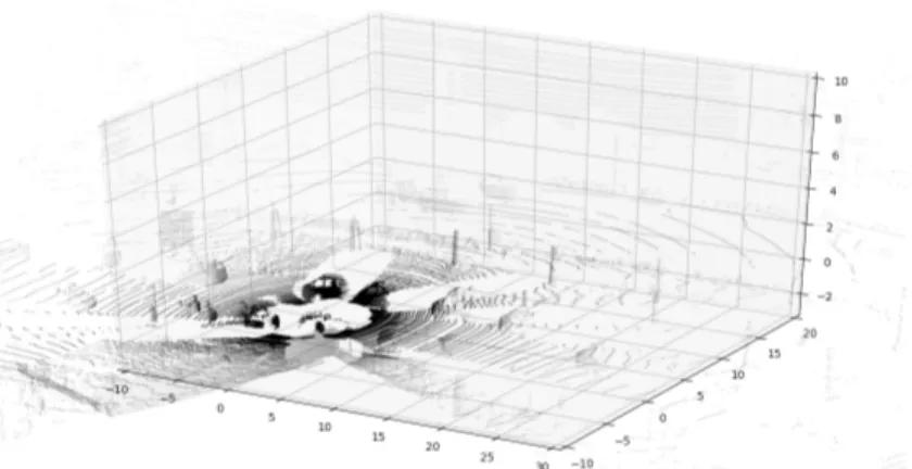
From this subsection onward the word ”data” refers only to the point clouds since our work is based on them.
The average number of points inside a point cloud is ⇠ 100.000, but not all the points can be considered interesting for our purpose. The task to solve is to recognize and detect cars and vans in front of ”our car”, but the data are recorded from all around the LIDAR sensor (see for example Fig.20). Moreover, the labels are referred only to the object in front of the camera. Thus, the first step to do is to remove the unused points in order to reduce the amount of data and, more important, to reduce the input size of our network (discussed later on).
To get this new visualization of the point cloud we have taken the frustum view of the point cloud using the corresponding image. Then, applying the right transformation matrices from the calibration files and cropping the point cloud sizes to the image sizes we obtained a new point cloud showed in Fig.22:
Figure 22: KITTI frustum view point cloud 3.3.1 Class labeling of Lidar points
Our first data transformation consists in adding a new column which indi-cates whether the point belongs to an object of interest or not. Therefore, we seek all points inside the annotated 3D bounding boxes and label them as interesting points. Exploiting geometry, a general point (x, y, z) is inside an axis-aligned box if:
xmin < x < xmax (18)
ymin < y < ymax (19)
zmin < z < zmax (20)
Since the cars and the other objects are not aligned with the axis this ap-proach cannot be used, but a more general representation is required. So, let one vertex be expressed as O and A, B, C the three adjacent vertices, the point P = (x, y, z) and OA =! !A !O as the vector distance between O and A the new formulas are:
O·OB < P! ·OB < A! ·OB! (22) O·OC < P! ·OC < A! ·OC! (23) A graphical representation of the result is shown in Fig.23, with the points belonging to a car in blue:
Figure 23: Points of interest
Using this method we have kept track of all the points of interest and built our new dataset. This dataset is used in the first step of the thesis in which we have tried to do a point-wise classification of the point clouds. An exam-ple of the data is shown in the Tab.2.
X Y Z Class 52.385 0.936 1.996 0 35.726 1.134 0.982 0 41.112 7.765 2.213 1 32.456 4.836 1.337 2 22.733 3.110 3.701 0
Table 2: Classification dataset example
Here 0 depicts background points, while numbers greater than 1 show points belonging to one of the classes. The numbering is used later for evaluation purpose especially for the output visualization of the bounding boxes. 3.3.2 Computing the centroid
The second data transformation has been done to test new further features of our network and the main thing that led us to make changes was the feasibility to regress vectors. In particular, we added the centroids to our dataset. Specifically, we have stored the vector distance from each point of a car to its centroid. To get all the centroids we computed the 3D center of the bounding box.
A view of one example result is shown in Fig.24.
Figure 24: Centroid of a car
have the vectors from each point of the car to the centroid and in red we have the car points.
Figure 25: Centroid of a car with vectors Tab.3 shows the structure example of a input file of the network.
X Y Z Class Xctd Yctd Zctd 52.385 0.936 1.996 0 0 0 0 35.726 1.134 0.982 0 0 0 0 41.112 7.765 2.213 1 2.802 5.001 1.112 32.456 4.836 1.337 2 -1.489 4.330 2.112 22.733 3.110 3.701 0 0 0 0
Table 3: Centroid vectors dataset example
We can see that in the correspondence of the Class value 0 the vector’s centroid information is absent, on the contrary, in the labelled objects the coordinates Xctd, Yctd and Zctd store the information of the distance vector between that point and the centroid of the object it belongs to.
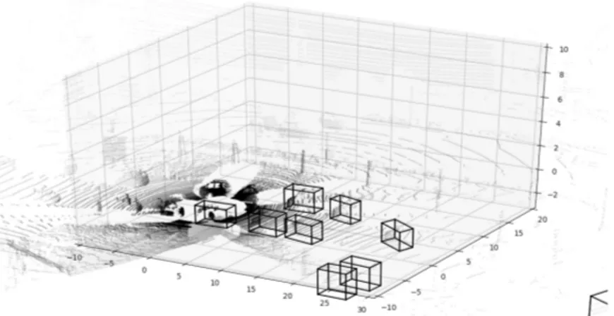
3.3.3 Annotation of 3D Bounding Box
The third and last manipulation of the dataset consists of removing the cen-troid information and adding the distance vectors from the points to the eight corners of the bounding box. Using the same car of the example in Fig.25
Figure 26: Example vectors from point cloud to a vertex
and focusing our process only for one vertex the result is shown in Fig.26. Each red point is a car point and the green lines are the vectors which go from the point to the corner.
Another transformation that has been made concerns the objects to be recog-nized. Since the pedestrian and the bicycle are very small object with respect to the whole point cloud it is really tough to detect them. Even trams and trucks are difficult to recognize, so what we did was to remove all of these objects and leave only cars and vans. To make this possible we have nulli-fied all the rows in the dataset corresponding to this list of objects making them not interesting for our network. Moreover, the number of points of a car depends on the distance between it and the sensor; if the car is very far away the number of points belonging to it could be also equal to one. For this reason, we have chosen to remove all the cars and vans with less than 50 points.
X Y Z Class Xbb (x8) ... Ybb (x8) ... Zbb (x8) ... 52.385 0.936 1.996 0 0 ... 0 ... 0 ... 35.726 1.134 0.982 0 0 ... 0 ... 0 ... 41.112 7.765 2.213 1 1.802 ... 2.003 ... -3.211 ... 32.456 4.836 1.337 2 2.349 ... -1.230 ... 3.452 ... 22.733 3.110 3.701 0 0 ... 0 ... 0 ...
Table 4: Bounding boxes dataset example
The labels Xbb, Ybb and Zbb regard the coordinates of the bounding box which are stored as the eight X coordinates, then the eight Y coordinates and then the eight Z coordinates. In detail, the first triplet of them (which means first X, first Y and first Z) represents the vector distance between that point and the first corner of the bounding box and so forth.
The full numbering of corners is shown in Fig.27.
4
Project and Solution
In this chapter we talk about the three steps of our proposed solution for the task, giving an explanation for the choices we made. In particular in sec. 4.1 we explore the classification network. In sec. 4.2 we extend the solution to the centroid vector estimation and finally in sec. 4.3 we talk about the final model.
4.1
Classification
In this part, we have performed the first experiments with the TensorFlow library and we have built the foundations of our final network. As afore-mentioned in sec. 2.2.6 our architecture is built with 6 convolution layers followed by other 6 deconvolution layers. Our approach for the classification task uses a simple conv-deconv network made from scratch as follows:
Figure 28: Classification network
The input of our network are batches of 8 entire point clouds, with a number of points down-sampled at 13545, so the input shape is [8, 13545, 3]. The 13545 points in input has not been picked randomly, but it is equal to the size of the smallest point cloud obtained after the transformation process in sec. 3.3. To downsample the point cloud to the required input size, we have chosen to remove the specific amount of points in surplus from the points labelled as not interesting (class label 0).
last dimension equal to 1, since the output prediction could be either 0 or 1. In specific, the shape of the output tensor is [8, 13545, 1]
In detail each layer is:
Name Kernel size Stride Padding Input channels Output channels BN Activation
conv1 5x5 1 same 1 128 Y ReLU
conv2 5x5 1 same 128 128 Y ReLU
conv3 3x3 2 valid 128 128 Y ReLU
conv4 3x3 1 same 128 256 Y ReLU
conv5 3x3 1 same 256 256 Y ReLU
conv6 1x1 1 same 256 256 Y ReLU
dconv1 1x1 1 same 256 256 Y ReLU
dconv2 3x3 1 same 256 256 Y ReLU
dconv3 3x3 1 same 256 128 Y ReLU
dconv4 3x3 2 valid 128 128 Y ReLU
dconv5 5x5 1 same 128 128 Y ReLU
dconv6 5x5 1 same 128 1 N /
conv out 1x1 1x3 same 1 1 N /
Table 5: Classification network parameters
Here, the word ”same” in the padding means that we add enough zeros, such that the shape of the output is equal to the shape of the input. On the contrary ”valid” means no padding so the output shape is reduced. In fact, we use ”valid” when the size of our tensor changes.
We have made a test on a training set composed of one point cloud repeated several times to try if we can successfully overfit to the desired outcome. To train it we have used as error loss function a sigmoid cross entropy since the output is binary. We have trained it for 80 epochs with a learning rate of 0.001 using an Adam optimizer to update the weights. Fig.29 shows the results.
The image shows really bad results. This is due to an imbalanced dataset with a large number of zeros and a few ones. For instance taking the example point cloud of the image 22 the total number of zeros is 10626 and the ones are 2919. To overcome this problem we have split the error formula into two factors called ”positive error” and ”negative error”. Basically, the negative error computes the error for the class label 0 and the positive error is used for the class label 1. In particular, for each factor we have counted the total
Figure 29: Classification result
number of zeros and ones in the label column, we have then summed up the error computed with the sigmoid cross entropy in the corresponding of zeros and ones to get the ”positive error” and ”negative error”. Finally, we divide these two errors for the corresponding total number of sample.
An example in pseudo-code is:
d e f c l a s s i f i c a t i o n l o s s ( l a b e l s , p r e d i c t ) : t o t p o s i t i v e = count ( l a b e l s , 1 ) t o t n e g a t i v e = count ( l a b e l s , 0 ) l o s s = s i g m o i d c r o s s e n t r o p y ( l a b e l s , p r e d i c t ) l o s s p o s i t i v e = m u l t i p l y ( l o s s , l a b e l s ) l o s s p o s i t i v e = sum ( l o s s p o s i t i v e ) l o s s p o s i t i v e = d i v i d e ( l o s s p o s i t i v e , t o t p o s i t i v e ) l o s s n e g a t i v e = m u l t i p l y ( l o s s , 1 l a b e l s ) l o s s n e g a t i v e = sum ( l o s s n e g a t i v e ) l o s s n e g a t i v e = d i v i d e ( l o s s n e g a t i v e , t o t n e g a t i v e ) r e t u r n l o s s p o s i t i v e + l o s s n e g a t i v e
The formula of the loss is:
Lossclassif ication = Losspositive+ Lossnegative (24)
After this technique the results have improved massively as can be seen in Fig.30.
Figure 30: Classification result
Tests regarding the whole dataset have been carried out with the final model and their results will be discussed in sec. 5.
4.2
Centroid vectors regression
This section talks about the regression of the vectors distances between the points and the centroid of the object they belong to. The data structure of the input files is shown in sec. 3.3.2. To address this task we have used the same network as before, changing just the output layer to add the 3 output columns for the components of the vector’s coordinates.
The results shown in this subsection have been obtained using the same dataset composed of one point cloud as before.
To choose the right loss function we have performed several tests. In partic-ular, we have tried with three functions:
1. L2 loss function 2. L1 loss function
3. Smooth L1 loss function
The L1 and L2 loss functions have been already defined in sec. 1.5.1. The Smooth L1 loss is less sensitive to outliers than the L2 loss and is defined as:
L1smooth =
(
↵x2 |x| < threshold
|x| ↵ otherwise
with ↵ as a scaling factor usually set to 0.5, threshold usually set to 1 and |x| as the normal L1 loss. This formula means that after computing the L1 loss, for each element check the loss value and if it is below the threshold square it otherwise no action.
To compute the loss we have used the same method in the classification task slitting the error in ”negative error” and ”positive error”. The final loss is:
Loss = Lossclassif ication+ Lossvectors (25)
The next three images (Fig.32, Fig.33 and Fig.34) show the results respec-tively for L2 loss, L1 loss and Smooth L1 loss in one car of the point cloud.
Figure 32: L2 loss function
Figure 33: L1 loss function
In these figures, the green dots show the ground-truth and the red dots show the prediction. This ”red car” is obtained adding to the real centroid all the vectors predicted by every single point of the cloud. Looking at these images we can immediately see that the L2 loss function is the one that has the worse results. Between the L1 loss and Smooth L1 loss is a bit more com-plicated to see who is the best, but empirically, we discovered that smooth L1 provided the best results. The ”red car” plotted using this loss function follows the shape of the ground-truth in a better way.
4.3
Bounding boxes regression
This task is the main focus of the thesis, therefore, the model proposed and the choices taken have to be considered as part of the final solution.
Our decision to do a point-wise prediction enforcing the points to regress the vector direction to the corners has three main advantages. Firstly, the network learns a 3D region which depends on the size of the object. Sec-ond, more important, even if a car has an occluded part, the corners of the bounding box can be predicted by the visible points. Lastly, we have less features than regress the rotation, the translation and the dimensions of the boxes like most paper do.
In a first attempt we have used the same model as the previous tasks, just changing the output size tensor in order to use the 24 bounding boxes coor-dinates.
We have trained it for 250 epochs using the same design choices as before regarding learning rate and optimizer. As loss function, we have used the same technique with positive examples and negative examples ending with a final loss described as
Loss = Lossclassif ication+ Lossboundingboxes (26)
Even if the model performed well in the previous experiments in the bound-ing boxes regression task its results looked very bad.
A couple of examples are shown in Fig.36.
Figure 36: Example result first bounding boxes prediction approach Even tuning the various parameters mentioned before like learning rate, op-timizer and batch size, our network could not achieve good results. This meant that our model had to be changed trying to build a new one more robust and more powerful.
A first modification we have thought about was to go one step deeper with the encoder block in order to capture better features. After that, the other big change we have done was to add the skip connections from the layers in the encoder block to the ones in the decoder block. We have chosen to add these links between layers, inspired by the good results of [53], [54] and [55], in order to enhance the features learned by the network and ease the optimization. The final model is shown in Fig.37.
Figure 37: Final network
This model has the same input as the others, a tensor of shape [8, 13545, 3] and the output of shape [8, 13545, 25]. The 25 numbers are 1 for the classi-fication label, either 0 or 1 as explained in sec. 4.1. The 24 others are the coordinates x, y, z for the vectors from the specific point to all the 8 corners of the bounding box. The specification of the layers is reported below in Tab.6.
We have run it on the same overfit task to see if this model could achieve better results.
Figure 38: Example result bounding boxes prediction using the new final model
Name Kernel size Stride Padding Input channels Output channels Activation Dropout
conv1 5x5 1 same 1 64 ReLU /
conv2 5x5 1 same 64 64 ReLU /
conv3 3x3 2 valid 64 128 ReLU /
conv4 3x3 1 same 128 128 ReLU /
conv5 1x1 2x1 valid 128 256 ReLU /
conv6 1x1 1 same 256 256 ReLU /
dconv1 1x1 2x1 valid 256 128 ReLU /
conc1 / / / / 256 / /
conv conc1 3x3 1 same 256 128 ReLU /
dconv2 1x1 1 same 128 128 ReLU /
conc2 / / / / 256 / /
conv conc2 3x3 1 same 256 128 ReLU /
dconv3 3x3 2 valid 128 64 ReLU /
conc3 / / / / 128 / /
conv conc3 3x3 1 same 128 64 ReLU /
dconv4 5x5 1 same 64 64 ReLU /
conc4 / / / / 128 / /
conv conc4 3x3 1 same 128 64 ReLU 40%
conv7 1x1 1 same 64 25 / /
conv out 1x3 1 valid 25 25 / /
Table 6: Bounding box network parameters
The results shown in Fig.38 looks really better than the previously obtained with the old model. Since every point predicts a vector from itself and the corners we have a lot of possible corners’ positions. For this reason, at the moment, we extract the final bounding box computing the median of all the coordinates of the corners.
From this bunch of pictures it’s possible to note that as the number of car points increases, the prediction improves.
Once we have found a good model we could proceed doing experiments with the entire dataset and see how our network performs in a real task.
4.3.1 Robust corner detection
To enhance the bounding boxes prediction, we have chosen to forecast the corners position in the space building a RANSAC[45] method to select the vectors which count in the voting for a corner. Briefly, RANSAC (RANdom
SAmple Consensus) is a technique to estimate parameter in a model by random sampling the data. It is an iterative and non-deterministic algorithm which implements a voting scheme to get rid of outliers. Precisely, for this reason, an advantage of RANSAC is its ability to do a robust estimation of the model parameters. In our solution RANSAC is applied with a max iteration parameter of 10. In each iteration the algorithm selects at most 5 vectors for each corner and computes the centroid point of all the destination point of the vectors. Giving that point RANSAC selects and count all the other vectors which casts a prediction in a confidence region of the centroid. At the end the centroid with more votes is selected to be the output.
4.3.2 Clustering for real application of the model
Moreover, in order to use our network in real tasks we had to add something more after the prediction output from the model. Our network focuses on two tasks; one is the classification of the points of interest and the other the bounding box regression. All the images showed before had the ground-truth bounding box plotted to see how the network predicts good with respect to the true coordinates. In a possible deployment in a car the system does not have the label, so the ground-truth for the point and for the bounding box. The classification result just categorizes the point as 0 or 1, but not specify to which car or van it belongs to. To solve this issue we have applied a clustering method to all the points labelled as 1, trying to find the cars in the scene.
The clustering algorithm we have chosen is DBSCAN[10]. Our choice is forced by the fact that we do not know how many objects we have in the scene and one of the advantages of using DBSCAN is this, we don’t need to tell the algorithm the number of clusters to find. Additionally, it can identify outliers as noise and skip them instead of adding in a known cluster similar to what mean-shift[9] does.
4.3.3 Other improvements to our model
Fig.39 show clearly that the boxes predicted are not exactly squared but have some skewed edges. In order to have a better visualization we have chosen to apply a rectification process to our predictions. To be able to draw such boxes we first compute the length, width and height for all boxes calculating the center di↵erence between opposite faces. We then move them to (0, 0, 0)
in order to use SVD[56] to solve least squares applied on the corners and get the rotation. Finally, we create the boxes uses those sizes and move them back to the original position.
Figure 39: Cars with not rectified bounding boxes
In addition, to improve the results, we have applied a geometric filter to remove outliers after the clustering. We have seen that outliers have bounding boxes which are not rectangular, they are just 8 corners drew randomly. An example is shown in Fig.40
Figure 40: Example of acute angled corner
To remove such objects we apply a filter to check all the angles between the corners and if one or more is less than 60 , then the entire object is removed.
5
Experiments
In this section, we show how the model is trained explaining the design choices we took. Later we show both qualitative and quantitative results. All the experiments are carried out using Python 3.6 and TensorFlow[57], running on a NVIDIA Titan X GPU.
5.1
Data Augmentation
After the entire process of data preparation in sec.3.3 the total number of point clouds has decreased from 7481 to 5760. This happened because we chose to remove all the point clouds without cars. We have then split the dataset into 5696 files for the training and 64 for the evaluation. Since the task was very challenging and the number of training sample was very small we have chosen to adopt a data augmentation process on the fly. In particular, we applied mirroring of the point clouds and introduced noise. With this augmentation, the size of the input dataset ended up in ⇠ 17000 point clouds, which is not that much but better than before.
5.2
Network configuration
The training has been executed using the momentum optimizer with momen-tum equal to 0.9, a learning rate of 0.001, dropout of 40% and the gradient capped to 5 to stabilize optimization. We have trained the model for 250 epochs in a Titan X GPU evaluating the classification accuracy and preci-sion after each epoch. We also have evaluated the quality of the training process displaying images of the bounding boxes every 20 epochs.
5.3
Results
5.3.1 Classification results
After a training of 250 epochs we plotted the error loss curve for the three di↵erent augmented input of before; normal point clouds, mirrored point clouds and noised point clouds. We have also tracked the error during the evaluation step to be aware of possible overfit problems. The plots have rea-sonable trends which means that our network works properly. The results are shown in Fig.41.
Figure 41: Error curves of training phase
The error trend in the evaluation set goes down as for the other errors plots which signalizes that we are able to generalize to unseen data.
Even the results on classification accuracy and precision are good, Fig.42 and Fig.43 show the curves.
Figure 43: Precision of interesting points
The Fig.42 shows the trend accuracy for both classification of zeros and ones. The top value of the accuracy reaches 96.71% after 246 epochs. What’s important for us is the plot of the precision value (Fig.43) because it tells us how many true ones are correctly classified over all the ones predicted by the network. The maximum is reached in the epoch 240 with a precision value of 84.5%.
5.3.2 Bounding box results
A couple of example results is shown regarding the bounding box prediction is shown in Fig.44.