end-point detection of a deformable linear object from visual data

(1)

ALMA MATER STUDIORUM

UNIVERSITY OF BOLOGNA

School of Engineering

Master Degree in Automation Engineering

Master Thesis

End-point Detection of a Deformable Linear Object From Visual

Data

CANDIDATE:

SUPERVISOR:

Masood Roohi Gianluca Palli

CO-SUPERVISOR:

Riccardo Zanella

(2)

To Kamal and Safieh

my guardian angles

(3)

“ La natura universale questo fa: sposta le cose, le trasforma, le prende da

una parte e le porta da un’altra. Tutto è mutamento, ma ogni cosa è distribuita

in modo armonico ed equilibrato, sicché nulla d’insolito può accadere che non

rientri in quest’ordine, e nulla dobbiamo temere di nuovo.”

Marco Aurelio, A sé stesso, VIII, 6; 2008

(4)

Abstract

In the context of industrial robotics, manipulating rigid objects have been studied quite deeply. However, Handling deformable objects is still a big challenge. Moreover, due to new techniques introduced in the object detection literature, employing visual data is getting more and more popular between researchers. This thesis studies how to exploit visual data for detecting the end-point of a deformable linear object. A deep learning model is trained to perform the task of object detection. First of all, basics of the neural networks is studied to get more familiar with the mechanism of the object detection. Then, a state-of-the-art object detection algorithm YOLOv3 is reviewed so it can be used as its best. Following that, it is explained how to collect the visual data and several points that can improve the data gathering procedure are delivered. After clarifying the process of annotating the data, model is trained and then it is tested. Trained model localizes the end-point. This information can be used directly by the robot to perform tasks like pick and place or it can be used to get more information on the form of the object.

(5)

List of Figures

1.1 Perceptron, the fundamental building block of a neural network. . . 9

1.2 Common utilized activation functions. . . 10

1.3 Multi-output neural network with a single hidden layer[3] . . . 11

1.4 Every region of the input influences only one single neuron in the hidden layer[2] 12 1.5 General architecure of a convolutional neural network structured for classifica-tion[5]. . . 13

2.1 Bounding boxes with anchor boxes and location prediction. The width and height of the box are predicted as offsets from cluster centroids[15] . . . 17

3.1 Samples from the training dataset. . . 20

4.1 Key point matching between first frame and nth frame. . . 22

4.2 A successful and a failed bounding box transfer in different frames. . . 23

6.1 Loss and validation loss variation over the course of training. . . 27

6.2 Precision-Recall curve of the model on the testing dataset. . . 28

6.3 Predictions of the model on the testing dataset. . . 29

6.4 Predictions of the model on the scenes with different backgrounds with respect to the training. . . 30

6.5 Predictions of the model on the scenes with different backgrounds with respect to the training. . . 30

(7)

Introduction

Industrial robots are capable of performing wide variety of tasks including pick and place, assem-bly, and etc. Handling rigid objects by robots is well studied and practiced. However, working with and manipulating deformable objects is still challenging. The challenge arises with the uncertainty of the work-piece form. This also can lead to difficulty in sorting the work-pieces. This study is focused on deformable linear objects (DLO) such as cables, ropes, etc.

A big portion of the manufacturing industry like car manufacturing, home appliance, and industrial machines require to automatize DLO manipulation in the production process. De Gregorio et al [7] have done a semantic segmentation and model estimation on DLOs starting with detection of DLO’s endcap using a convolutional neural network. De Gregorio et al [6] used the same algorithm in another research integrating the DLO segmentation with inserting it in a specific position. Axel Remde et al [17]studied picking-up a cable with Industrial robots. In their study, position of the cable was approximately known and it was hanging freely in a gallows. So, there was no problem of detection or uncertainty of form involved. In a more sophisticated work, Koo et all [11] studied the problem of automatically assembling wire harness. Fukiji et al [10] propose a method to recognize the topological relationship between multiple cables by using image sensors. Nakagaki et al [14]propose method for inserting a flexible beam into a drill. Different from other researches, in this work, the contact force between the beam and drill is detected by measuring deformation of beam with vision sensor.

The general aim of this thesis is to detect the tip of a rope to perform a pick and place operation in future projects. Detection will be carried out by a convolutional neural network (CNN). The key concept in using neural network is that instead of defining a set of features, like it is done in machine learning algorithms, network will learn the features from a set of raw data. Not every architecture of neural networks is practical enough for this purpose. In a dense neural network, each hidden layer is densely connected to its previous layer meaning every input is connected to every output in that layer. Assuming the data is a RGB image which is three 2-dimensional matrices, it will be collapsed down into a 1-2-dimensional vector so it can be fed through the dense network. Every pixel in that 1-dimensional vector will be fed into the next layer. Therefore, the very useful spatial structure in the image will be lost. Moreover, there will be huge number of parameters because the network is densely connected. CNN helps to use the spatial structure in the input to inform the network and also reduce the number of required parameters.

(8)

LIST OF FIGURES 8 In order to train the network and detect the object, an algorithm called YOLO is used. YOLO applies a single neural network to the full image. It divides the image into regions. Then, it predicts the bounding boxes and computes probabilities of each one.

The theory of the neural networks is described in the first chapter. In the following chapter, a brief explanation is given on how YOLO operates. Then, the data gathering procedure is explained in chapter three. Labelling procedure is clarified in the fourth chapter. Process of training is put into words in chapter five. Results are laid out in chapter six followed by the conclusion.

(9)

Chapter 1 Neural Networks

1.1 Basic Structure of a Neural Network

The idea of neural networks is inspired by the operation of neural system and brain in humans body where billions of neuron cells are connected to each other in order to process data in parallel. Language translation and pattern recognition softwares are the well known examples where researchers succeed to execute the idea of neural networks on the computer[22].

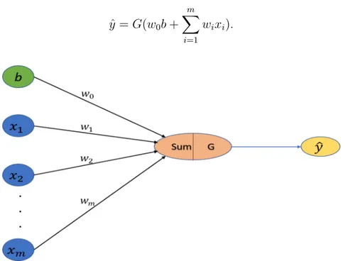
An artificial neural network consists of an input layer of nodes, one or two hidden layer of nodes, and final layer of output nodes. Inputs to and outputs from a neural network can be binary or continuous. This feature confers a wide range of applicability to neural networks.The fundamental building block of a neural network is called perceptron. Figure 1.1 depicts the forward propagation of information through a perceptron. In this figure, b is the bias, G is the nonlinear activation function and ˆy can be written as

ˆ y = G(w0b + m ∑ i=1 wixi). (1.1)

Figure 1.1: Perceptron, the fundamental building block of a neural network.

(10)

CHAPTER 1. NEURAL NETWORKS 10

(a) Sigmoid function (b) tanh function (c) ReLU function

Figure 1.2: Common utilized activation functions.

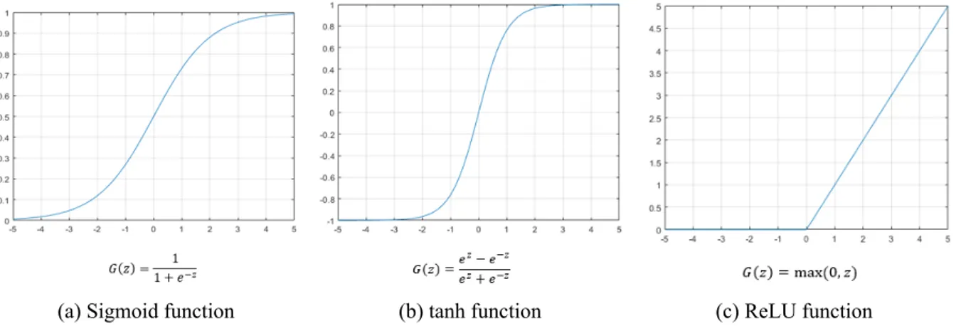
Role of the activation function is to introduce non-linearity into the network. No matter how deep is the network, if a linear activation function is used, the network will only compose bunch of lines on top of each other and it will yield another line. By introducing non-linearity, neural network allows one to approximate arbitrarily complex functions and this is what makes neural networks extremely powerful. There are several types of activation functions which are commonly used in the neural networks. Figure 1.2 presents three of these common functions. The purpose of the bias term is to provide the ability to shift the activation function to left or right, regardless of the inputs.

To construct a multi-output neural network, it is enough to simply attach perceptrons to each other vertically as shown in the Figure 1.3. This figure shows a neural network with single hidden layer. It is called hidden layer because unlike the inputs and outputs, it is not directly enforced or observable. Assuming that the bias is one, equation 1.3 gives the outputs of the network. zi = w (1) 0,i + m ∑ i=1 w_j,i(1)xj (1.2) ˆ yi = G(w (2) 0,i + d1 ∑ i=1 w_j,i(2)G(zj)). (1.3)

1.2 Training a Neural Network

It is possible to set up a neural network with several inputs and hidden layers and initialize the weights and biases. If the network is fed at this step by inputs, it won’t be able to predict the right output because basically the network does not know anything about the relation between input and the correct output. In other words, the network is not trained. Similar to human learning by examples, a neural network is trained by presenting to it a set of input data called training set and then compare the output with the real one to find a way to adjust the weights. In fact the

(11)

Figure 1.3: Multi-output neural network with a single hidden layer[3]

goal is to find the weights which deliver the lowest loss. Mathematically speaking

W∗ = arg min W 1 n n ∑ i=1

L(f (x(i), W ), y(i)) = arg min

W

J (W ), (1.4)

where W is the weight matrix, f is the predicted output or ˆy, and y is the real output. So, for any

value of W we can compute the loss function, J (W ). Then, after initializing the network with a random set of variables, one should look for the direction that will reduce the loss. To this end, slope of the function can be observed. Therefore, the gradient of the loss with respect to each of the weights should be computed to find the direction of the maximum descent. During training, this process is repeated over and over until the loss converges to a local minimum. In a nutshell:

1. Random weight initialization

2. Loop to convergence

• compute the gradient, ∂J (W )_∂W

• adjust the weights W − η∂J (W )_∂W → W 3. Return the weights.

This is called the backpropagation algorithm.

o create a deep neural network, the idea is basically stacking on more of these hidden lay-ers.The ancient term “deep learning” was first introduced to machine learning by Dechter[8], and to artificial neural networks by Aizenberg et al [1]. Subsequently, it became especially pop-ular in the context of deep neural networks[19]. In 21st century, by the help of more powerful CPUs and then new GPUs, deep neural network has shown that it can outperform the classic models. Although containing several hidden layer is recognized as the main difference between

(12)

Figure 1.4: Every region of the input influences only one single neuron in the hidden layer[2]

deep learning and the so called shallow learning, more outstanding difference is that deep learn-ing methods derive their own features while in the antecedent models, hand-engineered features should be provided for the model.

1.3 Convolutional Neural Networks

Today, to give the machines a sense of vision, convolutional neural networks are widely used. The general approach is to learn the visual features directly from data and learn a hierarchy of these features so that they can reconstruct a representation of what makes up the final class label. Neural networks are able to learn the features directly from the visual data if they are structured cleverly and correctly.

As it was mentioned in the introduction, employing dense neural network for the purpose of computer vision would be very costly computationally speaking and some information regarding the spatial structure will be lost. To maintain the spatial structure, CNN connects patches of the input to a single neuron in the hidden layer. This concept is illustrated in Figure 1.4.

Window of the patch slides with a determined step size (stride) to define all the patches. In order to learn the features, the connections of the pixels within the patch and the node in the hidden layer must be weighted. Thus, the node at the hidden layer will have the weighted sum of the pixel values belonging to the connected patch. This operation is called convolution and the weighted windows sliding on the image are called filter. By sliding different filters on top of the image, different features will be extracted. Thus, the output layer of a convolution is not a

(13)

CHAPTER 1. NEURAL NETWORKS 13 single image (feature map) but rather a volume of images representing all of the different filters. Need to mention that each node in the hidden layer, will compute a weighted sum of it’s input from the corresponding patch plus a bias and then it will apply a nonlinear activation function which is commonly ReLU. Non-linearity allows the network to deal with non-linear data and introduces complexity into the learning pipeline. Note that each node in the hidden layer is only seeing a single patch from the image. This property is called local connectivity.

After convolution layer, there is a pooling layer used to reduce the dimentionality of its input. In other words, role of pooling layer is to reduce the resolution of the feature map but keeping the features required for classification. Common technique for pooling is called maxpooling. The idea is one can slide a window over the feature map and takes the maximum value in the current window. If the window size be 2×2, pooling layer will discard three fourth of the feature map.

Normally, in a CNN there are multiple convolutional and pooling layers one after each other to derive the hierarchy of features. Final derived features are fed to a dense neural network to classify the input. Figure 1.5 illustrates the CNN architecture structured for classification.

Figure 1.5: General architecure of a convolutional neural network structured for classifica-tion[5].

(14)

Chapter 2 You Only Look Once: YOLO

What Image classification does is setting a class label to an image. There is another concept called object localization which is the act of drawing a bounding box around the object in the image. The goal in this project is object detection. Object detection combines image localization and classification. The main families of deep learning object detection algorithms are ”Region-based convolutional neural network” (R-CNN) and ”Yolo look only once” (YOLO). The utilized algorithm in this study is YOLO.

CNN architecture can be employed for the purpose of classification or regression. Earlier introduced algorithms like R-CNN repurpose classifiers for the detection. To perform object detection, these algorithms take a classifier for the object and evaluate it at various locations and scales in a test image. In fact, after receiving the input image, they propose several regions or candidate bounding boxes. The algorithm to select these regions can be different but in the main R_CNN this step extracts about 2000 regions. Then, CNN will be applied to each of these candidate regions to extract the features. Finally, Extracted features will be fed to a classifier model to label them as one of the known classes[4].

On the other hand, YOLO performs object detection as a single regression problem. In fact, original version of the YOLO was trying to directly regress the coordinates, width, and height of the bounding boxes. It was fast but it was not as precise as the competing algorithms. Object detection algorithms usually sample a huge number of regions in the input image and control if it contains a classified object or not. Then, they try to adjust the coordinates of the region to predict the bounding box more precisely. These predefined regions or bounding boxes are called anchor box. Faster R-CNN[18] and SSD[13] take these anchor boxes in three different scales and aspect ratios and compute offsets to the anchor boxes to predict boxes for the object. YOLO employed the idea of the anchor boxes but to make learning more simple for the network, they ran a k-mean clustering on the bounding boxes of the training dataset and came up with a set of dimension clusters.

In YOLO, input image is divided into a grid and to each grid cell a set of anchor boxes are associated with the same centroid. Then, it computes how much does the ground truth box overlaps with the anchor box and picks the one with the best IoU. So, it can now predict offsets

(15)

CHAPTER 2. YOU ONLY LOOK ONCE: YOLO 15 to the anchor box. In a nutshell, things to be predicted are

1. the location offset against the anchor box: tx, ty, tw, th.

2. Probability of the box containing an object.

3. Probability of the box belonging to any of the introduced classes: num_classes

Thus, for every anchor box (4 + 1 + num_classes) numbers are predicted and if the image is divided into a s× s grid and each cell of the grid had B anchor boxes, output would be a volume of size s× s × B × (4 + 1 + num_classes)[12].

These predicted values are used to derive the loss function value. Loss function in original YOLO is defined as [16] λcoord s2 ∑ i=0 B ∑ j=0 1obj_ij [(xi − ˆxi)2+ (yi− ˆyi)2]+ λcoord s2 ∑ i=0 B ∑ j=0 1obj_ij [(√wi− √ ˆ wi)2+ ( √ hi− √ ˆ hi)2] + s2 ∑ i=0 B ∑ j=0 1obj_ij (Ci− ˆCi)2 + λnoobj s2 ∑ i=0 B ∑ j=0 1obj_ij (Ci− ˆCi)2 + s2 ∑ i=0 1obj_i ∑ c∈C (pi(c)− ˆpi(c))2 (2.1)

Equation 2.1 can be interpreted as the sum of classification loss,Lcls and localization loss,

Lloc, and be rewritten as Loss = Lcls+ λcoordLloc[23] where

Lcls = s2 ∑ i=0 B ∑ j=0

(1obj_ij + λnoobj(1− 1objij ))(Cij− ˆCij)2 s2 ∑ i=0 1obj_i ∑ c∈C (pi(c)− ˆpi(c))2, Lloc= s2 ∑ i=0 B ∑ j=0 1obj_ij [(xi− ˆxi)2+ (yi− ˆyi)2+ (√wi− √ ˆ wi)2+ ( √ hi− √ ˆ hi)2]. (2.2)

Parameters of these functions are defined as following:

• xi, yi, wi, hi: coordinates of the predicted bounding box.

• ˆxi, ˆyi, ˆwi, ˆhi: coordinates of the ground truth bounding box.

(16)

CHAPTER 2. YOU ONLY LOOK ONCE: YOLO 16 • iobj_i j: Indicating if jth anchor box of the ithcell contains an object or not.

• ˆCij: Confidence score of the cell i with respect to box j.

• Cij: Predicted confidence score.

• ˆpi(c): Conditional probability of whether cell i contains an object of class c∈ C.

• pi(c): predicted conditional class probability.

First part of the Lcls can be interpreted as kind of a objectness loss meaning that network

can learn from this part to detect the region of interest. Also, by using the term (1− 1obj_i j), loss

is penalized for false positive predictions. λnoobj is a float between 0 and 1 to make sure that

the model is not dominated by cells that do not have object. Another point about Lcls is that,

this equation belongs the the original YOLO algorithm and in YOLOv3 they have used binary cross-entropy function instead of this sum of squared errors[15].

Moreover, it is mentioned earlier in this chapter that unlike original YOLO, YOLO9000 and YOLOv3 predict the offsets from the anchor boxes. Thus, to follow the notation introduced in YOLOv3, network predicts four coordinates for each bounding box, tx, ty, tw, th. Offset of the

cell from the images origin is (cx, cy) and anchor box has width and height pw and Ph. So, the

predictions correspond to [15] bx = σ(tx) + cx by = σ(ty) + cy bw = Pwetw bh = pheth, (2.3)

where bx, by, bw, and bh are absolute values of the coordinates with respect to the image origin.

Note that for example, txand ty are predicting the centroid with reference to the top-left corner

of the cell not the image. Figure 2.1 helps to clarify these notations.

Therefore, if the ground truth for some coordinate prediction is ˆt_∗, the error will be the ground truth value minus the prediction: ˆt_∗ − t_∗. Note that ground truth values can be derived by inverting equation 2.3.

(17)

CHAPTER 2. YOU ONLY LOOK ONCE: YOLO 17

Figure 2.1: Bounding boxes with anchor boxes and location prediction. The width and height of the box are predicted as offsets from cluster centroids[15]

(18)

Chapter 3 Data Gathering

For the purpose of training, labelled data or in this case labelled images as a dataset is required. Nowadays, there are a lot of collected and ready dataset provided in the Machine learning com-munities such as coco dataset which contains 80 classes like human, tree, car, etc., 80000 training images and 40000 validation images. Obviously, training dataset is not provided for every ob-ject. Therefore, a custom dataset is prepared. As a rule of thumb, it is suggested to store at least 1000 images for every class of objects to have a successful training. Also capturing 1000 photos either manually or even automatically by the help of a manipulator is frustrating. Moreover, it is mentioned 1000 images per class of objects, thus, 1000* n images where n is the number of classes are needed. To tackle this issue, instead of capturing photo, it is possible to shoot a video and then extract properly spaced frames.

Before starting to shoot the video, it is necessary to decide about the distribution of the data. In, other words, if the training dataset are captured in a specific condition or environment, then the model will be trained for that specific environment. Shooting angle, Lighting, background, and form of the object might be of the degrees of freedom to select. Considering the situation in which the model will be used can be helpful to decide about the data distribution. As such it is presumed that the image plane must be parallel to the plane that object is located at. Therefore, assuming the image plane is xy plane and the axis perpendicularly coming out of the image plane is the z axis, camera is free to move along all the axes and rotate around the z axis but it must not rotate around x and y axes. As camera moves uniformly, the extracted frames will be more clear images being less blurry. This end can be achieved by using a manipulator to move the camera around in a predetermined trajectory. At the moment of data collection for this study, there was no manipulator available. Thus, it was decided to shoot the videos by a smartphone and manually. However, it is imaginable how difficult it is to move the camera as smoothly as a manipulator. Therefore, Instead of the camera, object (basically the platform was moving) was decided to move. The deformable object is rested on a cardboard. It was possible to translate and rotate the cardboard in the xy plane; however, for translation along the z axis it was only possible to move the camera in a limited discrete set. As for the lighting, not a very strict standard was selected; however, it was tried to not do the shooting in a dark environment.

(19)

CHAPTER 3. DATA GATHERING 19 The word dark might be general, but the basic lighting was the morning daylight plus room fluorescent lighting because it could mimic the lighting condition in the lab where the model can be used.

Background was a random paintings of Jackson Pollock[9] glued to a piece of cardboard. Since content of these paintings have very random texture, they are suitable for domain random-ization[21]. Domain randomization helps one to bring the simulation or controlled environment close to the reality. The idea is that if a suitable randomness appears in the simulation, also real world would look like as a type of simulated environment. Also, it has been tried before and demonstrated that this choice of background provides good enough random features so the network will only learn the features of the object. Consider the case where background was uni-formly white. In this case since the object is black, probably network will learn that the gradient orientation at the edge of the object is always normal to the edge toward the background. It was possible to choose a uniformly textured background but this decision is made hoping to have the model more generalized with respect to the background.

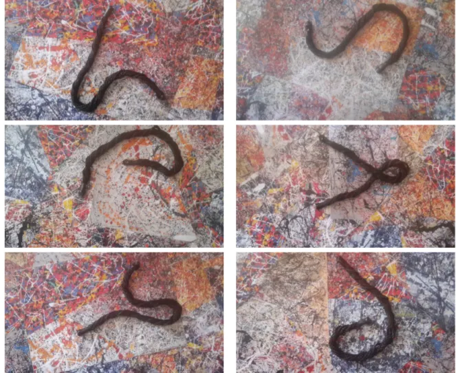
Another important point to consider about the deformable linear object is it is possible to shape a wide variety of curves. The point is not to find the object itself but its end-point. So, the form of the object should be variant to prevent the model from adapting to a unique form. Therefore, it was necessary to shoot several videos, where the object has different forms laying on different backgrounds. Figure 3.1 depicts some samples of the acquired dataset. Finally, about 5500 images from 7 videos got extracted to provide the training dataset.

It worth to mention that generating dataset did not happen in one trial. The point is although there is only one type of object which is the wiretip, a classification has been done based on the orientation of wiretip. In fact, the classification based on the orientation is done by the labelling tool that is used in this study. The tool demands user to determine the degree of discretization. For example, id one chooses to discretize the orientation with 10 degree bins, then there will be 36 classes of object. This means there is a requirement for about 36000 images and about 1000 images per class as training dataset. Otherwise, the model will be underfit. This is what happened at the first trial. Beside that, while shooting the video, the followed trajectories were not involving enough rotation and they were mostly translational movements.

Considering these points, second trial was much more successful but not good enough. The problem was that extracted frames from the videos were not properly spaced. In other words, frames were chosen too much close to each other and they were very similar. Although the algorithm prevents the model from overfitting, this kind of dataset implicitly makes the model overfit because it is getting traind by a bunch of images which all are very similar together. Addressing this issue by down sampling, finally a suitable dataset was provided. In fact the problem is that it is required for models to learn representations from the training data that can be generalizable to unseen test data.

(20)

CHAPTER 3. DATA GATHERING 20

(21)

Chapter 4 Labelling

Labeling In Supervised learning, the learner receives a set of input and output pairs as training data and then makes prediction for the test data which are unseen before. This is the most common scenario associated with classification, regression, and ranking problems. Therefore, data is required to be labeled or annotated. To do so, coordinates of four corners of a rectangle bounding the object (called bounding box) should be derived and stored along with the class of the object to provide the ground truth for training and also testing. This procedure should be followed for each object in the image and for all of the images in the training dataset.

Labeling can be carried out manually or automatically by the help of a software. Usually for the purpose of deep learning, a gross amount of data is required and as mentioned before, in this study 5500 number of images are used. Labeling this number of images manually would be extremely time consuming. Therefore, a novel software called Loop is used to label all the training images.

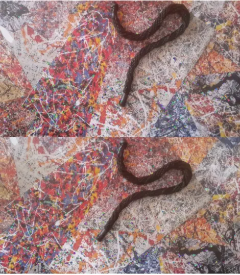
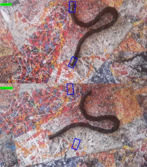
LOOP is a software developed by the researchers of the University of Bologna to reduce the human intervention during the process of annotation. It has been used numerous times for the purpose of deep learning application in industrial robotics and resulted very effectively. In case the requirements are met, working with LOOP is easy. In the first frame of each video, a box should be drawn around the considered object. Then, LOOP finds as many key points as it is determined and frame by frame, it follows the key points to transfer the box. To repeat the algorithm, monitoring by human is required because it is possible for the tool to miss the correct transformation. This can happen in the case of lighting variation, change in the scene or any other thing that leads to missing a big number of key points. Figure 4.1 is representing the situation in which corresponding key points are found in first and nth _{frame. Also, Figure 4.1}

exhibits the interface of the LOOP and the case that it has missed the object.

(22)

CHAPTER 4. LABELLING 22

(23)

CHAPTER 4. LABELLING 23

(24)

Chapter 5 Training

First thing to do before starting to train is setting the hyperparameters. most of the parameters are optimize and already tuned in the YOLO algorithm. Therefore, limited number of hyperpa-rameters including learning rate, batch size, and number of epochs where chosen to be tuned. There are different methods to choose the hyperparameters including random search and grid search; however, in this study, tuning procedure was performed manually and empirically. This procedure is performed based on the general ideas introduced in the literature.

The learning rate can be interpreted as the step size of the weight adjustment. The smaller is the learning rate, smaller the weight change after an iteration. As it was mentioned earlier, in YOLO architecture training is a gradient descent optimization algorithm. If learning rate is given a very large value, training will be faster; however, it might not converge toward an optimum solution. On the other hand, very small learning rate will lead to a very time consuming training. Regarding these behaviors, normally learning rate is not held constant and it is beneficial to decay during the training process. Usually, this is done by two type of methods named learning rate schedules and adaptive learning rate methods. Learning rate schedules are predefined sched-ules which may decay based on time or step or decay exponentially. The challenge of tuning the schedule in advance can be removed by the help pf adaptive learning rate methods including Adagrad, Adadelta, RMSprop, and Adam. YOLO employs Adam to tune the learning rate. In fact, Adam is extended version of stochastic gradient descent optimization algorithm. While in stochastic gradient descent learning rate is the same for all weights and does not change dur-ing traindur-ing, Adam “computes individual adaptive learndur-ing rates for different parameters from estimates of first and second moments of gradients”.

During training process, at every iteration a limited number of samples are chosen randomly to be used as the input data. This limited number of samples is the batch size. By increasing the model size, there will be less amount of GPU memory available for the input samples because the number of weights and calculations increases as well. Besides that, extremely large batch size leads to overfitting. Thus, upper limit of batch size is mainly influenced by the available GPU memory and the performance. On the other hand, very small batch size elongates the training time to converge. That’s because weight update is done based on the batch of input samples

(25)

CHAPTER 5. TRAINING 25 and as it gets smaller, generality of the input may decrease and weights change will be more fluctuating. Also, Smith[20] has shown that increasing batch size increases the test accuracy. Unfortunately, in the current study, the available GPU memory did not allow to increase the batch size to more than 8. Thus, at the end, there were not a lot of options.

One epoch is a step in which all the dataset propagates through the network. The right number for the epoch is the one that prevents underfitting and overfitting. There is a basic technique called regularization to overcome the problem of overfitting in neural networks. What this technique does is that it discourages the model from learning complex information which are not generalizable very much. The most popular regularization technique in deep learning is the idea of drop-out. The idea is during training randomly a set of activations in the hidden nodes are set to zero. The idea is extremely powerful because by lowering the network capacity it prevents the network from building memorization channels in which it tries to just remember the data instead of learning. In fact, drop-out wipes out a portion of data and consequently helps the network to generalize and build a more robust representation of its prediction.

Another regularization technique is early stopping. As mentioned earlier, training a network is basically an optimization problem and the goal is to minimize the loss. As training goes on, loss function value over training and test dataset should decrease. Eventually, there will be a point in which loss value of testing dataset diverges from the one corresponding to training dataset. Naturally, the model will always fit he training data because it is seeing the training data but testing data is unseen. Therefore, at some point model start to perform on training data much better than testing data. Early stopping identifies this point where loss starts to increase and diverge from the loss over training data.

YOLO employs both these methods to prevent overfitting. Therefore, the only burden is to choose the epoch number large enough in order to avoid underfitting. Since hyperparameter selection was empirically, several set of them have been tried and the set corresponding to the final training is:

• 15 epochs of initial training with batch size 4 and learning rate 1e− 4

• 85 epochs of main training (fine-tuning) with batch size 4 and learning rate 1e− 5 An interesting mutual phenomenon between a lot of deep neural networks which are trained on natural images is that, on the first layers, they all learn features similar to Gabor filters and color blobs. In other words, these features which are extracted at the first layers do not specifi-cally belong to a special dataset or task, but they are general in the sense that they are applicable to many datasets and tasks. This phenomenon is known as the transferability of the features. Yosinsky et al[24] have quantified how the transferability gap grows as the distance between tasks increase and it will be more extreme for transferring higher layers; however, they have demonstrated that even features transferred from distant tasks are better than random weights. Based on this behavior, YOLO can be initialized with its pre-trained model which is trained on

(26)

CHAPTER 5. TRAINING 26 the coco dataset. Since the features at first layers are more similar to each other when compar-ing different tasks, YOLO performs an initial traincompar-ing for the last layers, particularly the fully connected layers, while the first layers are frozen. Basically, this step is enough to obtain a not bad model. Then, to perform a fine tuning on the model in order to make it more specialized on the given task, another step of training is done where all the layers are engaged in the training.

(27)

Chapter 6 Results

6.1 Quantitative Assessments

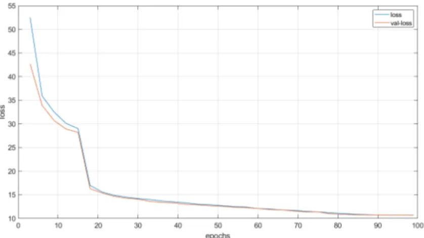
As it was stated earlier, during training the goal is to minimize the loss function. One may notice that after each epoch of training, YOLO releases two different losses. One is name val_lass which is the value of cost function for the cross-validation data and the other one is loss which is the value of cost function for the training data. Note that YOLO is given only the training dataset. Thus, a question may arise asking what is cross-validation data?

In the previous chapter, an approach called early stopping was introduced to prevent the model from overfitting. It was mentioned that when loss value on testing data diverges from the loss value on training data, training process is stopped. To this end, YOLO splits a portion of the training data to exploit it as the cross-validation data. Ratio of the split portion to training data is represented as val_split in the algorithm which takes a float between 0 and 1. Algorithm will store this portion of the training data and won’t perform training on it so it can compute the validation loss on this unseen data at the end of each epoch. Figure 6.1 depicts the variation of the loss and validation loss across 99 epochs of training. It was meant to be 100 epochs but YOLO early stopped at 99th epoch to prevent overfitting.

Figure 6.1: Loss and validation loss variation over the course of training.

(28)

CHAPTER 6. RESULTS 28

Figure 6.2: Precision-Recall curve of the model on the testing dataset.

To assess the model validity, mean average precision (mAP score) is calculated. To do so, 11 point interpolation technique is used[[https://www.cl.cam.ac.uk/teaching/1415/InfoRtrv/lecture5.pdf]]. Briefly explaining, first of all, Precision-Recall graph is plotted where Precision and Recall are defined as following:

P recision = true positive

true positive + f alse positive Recall = true positive

true positive + f alse negative

Then, precision is interpolated at 11 recall levels starting from 0.0 increasing with 0.1 step size until 1.0. Precision-Recall curve is supposed to be monotonically decreasing. So, precision at any point is the maximum of the last point and all the following points. Figure 6.2 shows how the curve is turned into. Finally, arithmetic mean of the 11 precision is calculated. Derived mAP score for the test data is 0.92.

6.2 Qualitative Assessment

The model performs reasonably well on the testing dataset images. Figure 6.3 exhibits some samples of the predictions. Usually the failed cases are the ones with a low quality and somewhat blurry appearance. Failure may happens because of the unstable lighting. Another problem is detecting multiple bounding box per object. This phenomenon is not very strange with YOLO. The issue is several predicted boxes are good enough to be detected. It can be handled by increasing the threshold on confidence score but it may lead to reducing the recall. So, a fair trade-off must be found.

Response of the model to the scenes with backgrounds different than the random back-grounds on training and testing datasets was tested too. The model was expected to respond

(29)

Figure 6.3: Predictions of the model on the testing dataset.

similarly to the testing datasets predictions. The result was not a total failure but it does not sat-isfies the expectation perfectly either. It is possible that the chosen backgrounds were not enough divers to set the requirements for domain randomization. After all, training dataset contains six different set of backgrounds. Figure 6.4 shows some of the predictions.

It was also of interest to check what would be the response of the model to other deformable linear objects beside the original rope which was used for the training. To this end, three shoe laces with different colors were used. After Observing several predictions, it seemed that the model has learned the color of the rope because it can detect the tip of the black and dark blue shoe laces but it never detects the tip of the white shoe lace. Figure 6.5 shows samples of these predictions.

(30)

Figure 6.4: Predictions of the model on the scenes with different backgrounds with respect to the training.

Figure 6.5: Predictions of the model on the scenes with different backgrounds with respect to the training.

(31)

Conclusion

In this thesis, neural networks and their application is the object detection is studied. It was tried to study the YOLOv3 algorithm very deep in order to get familiar with its potentials so it can be used effectively and as a matter of fact the results were strongly promising. Data collection procedure was a challenge to do and multiple points have learned by the author. To improve the dataset, it is suggested to provide more controlled environment particularly from the lighting aspect. Unstable lighting can play a very disturbing role during both training and testing. In this study, data were collected during daylight and it hardly can be called a controlled environment. It is better to collect the data during night and under particular lighting or collect a lot of data in different lighting situations.

Also, domain randomization helped to test the model on backgrounds different than on what it was trained but it was not totally successful. It is proposed to provide more diverse set of backgrounds to exploit the potential of domain randomization.

Moreover, the model was tested on objects different than what it was trained on and it showed some promising responses. If one wants to have a model that can detect a lot of different types of deformable linear objects, then by providing a few diverse target objects in the training dataset it seems an achievable goal.

Like Faster R-CNN, YOLO9000 and YOLOv3 model makes use of anchor boxes, pre-defined bounding boxes with useful shapes and sizes that are tailored during training. Using anchor boxes improved yOLO’s precision with respect to its original version. In this study, de-fault anchor boxes were used; however, it seems in case of defining particular anchor boxes for the custom dataset, the precision of the model can improve. Therefore, a k-means analysis can be carried out on the training dataset to define the custom made anchor boxes.

One more point that can improve the model is data augmentation. In this study it was not possible to capture images in different scales. Although YOLO itself carries out a multi-scale training, it will worth to try capturing images in different scales.

Finally, despite the fact that YOLOv3 performed very well in this project, today other ver-sions including YOLOv4 and YOLOv5 are introduced. So, it is advisable to try using these updated algorithms to have faster training and more accurate model.

(32)

Bibliography

[1] Igor Aizenberg, Naum N Aizenberg, and Joos PL Vandewalle. Multi-valued and universal

binary neurons: theory, learning and applications. Springer Science & Business Media,

2013.

[2] Soleimany Amini. MIT 6.S191 Deep Computer Vision. University Lecture, Available at http://introtodeeplearning.com/. 2020.

[3] Soleimany Amini. MIT 6.S191 Introduction to Deep Learning. University Lecture, Avail-able athttp://introtodeeplearning.com/. 2020.

[4] Jason Brownlee. A Gentle Introduction to Object Recognition With Deep Learning. Avail-able at https : / / machinelearningmastery . com / object recognition with -deep-learning/ (2020/07/13).

[5] Cezanne Camacho. Convolutional Neural Networks. Available athttps://cezannec. github.io/Convolutional_Neural_Networks/ (2020/07/13).

[6] D. De Gregorio et al. “Integration of Robotic Vision and Tactile Sensing for Wire-Terminal Insertion Tasks”. In: IEEE Transactions on Automation Science and Engineering 16.2 (2019), pp. 585–598.

[7] Daniele De Gregorio, Gianluca Palli, and Luigi Di Stefano. “Let’s take a walk on super-pixels graphs: Deformable linear objects segmentation and model estimation”. In: Asian

Conference on Computer Vision. Springer. 2018, pp. 662–677.

[8] Rina Dechter. “Learning while searching in constraint-satisfaction problems”. In: (1986).

[9] Famous Jackson Pollock Paintings. Available at https://www.jackson- pollock. org/jackson-pollock-paintings.jsp (2020/07/13).

[10] Rei Fujiki et al. “Autonomous recognition of multiple cable topology with image”. In:

2006 SICE-ICASE International Joint Conference. IEEE. 2006, pp. 1425–1430.

[11] Kyong-mo Koo et al. “Development of a robot car wiring system”. In: 2008 IEEE/ASME

International Conference on Advanced Intelligent Mechatronics. IEEE. 2008, pp. 862–

867.

(33)

BIBLIOGRAPHY 33 [12] Ethan Yanjia Li. Dive Really Deep into YOLO v3: A Beginner’s Guide. Available at https : / / towardsdatascience . com / dive really deep into yolo v3 a -beginners-guide-9e3d2666280e/ (2020/07/13).

[13] Wei Liu et al. “Ssd: Single shot multibox detector”. In: European conference on computer

vision. Springer. 2016, pp. 21–37.

[14] Hirofumi Nakagaki et al. “Study of insertion task of a flexible wire into a hole by using visual tracking observed by stereo vision”. In: Proceedings of IEEE International

Con-ference on Robotics and Automation. Vol. 4. IEEE. 1996, pp. 3209–3214.

[15] Joseph Redmon and Ali Farhadi. “Yolov3: An incremental improvement”. In: arXiv preprint

arXiv:1804.02767 (2018).

[16] Joseph Redmon et al. “You only look once: Unified, real-time object detection”. In:

Proceedings of the IEEE conference on computer vision and pattern recognition. 2016,

pp. 779–788.

[17] Axel Remde, Dominik Henrich, and Heinz Wörn. “Picking-up deformable linear objects with industrial robots”. In: (1999).

[18] Shaoqing Ren et al. “Faster r-cnn: Towards real-time object detection with region proposal networks”. In: Advances in neural information processing systems. 2015, pp. 91–99.

[19] Juergen Schmidhuber. Deep Learning. Available athttp://www.scholarpedia.org/ article/Deep_Learning (2020/07/13).

[20] Leslie N Smith. “A disciplined approach to neural network hyper-parameters: Part 1– learning rate, batch size, momentum, and weight decay”. In: arXiv preprint arXiv:1803.09820 (2018).

[21] Josh Tobin et al. “Domain randomization for transferring deep neural networks from sim-ulation to the real world”. In: 2017 IEEE/RSJ International Conference on Intelligent

Robots and Systems (IROS). IEEE. 2017, pp. 23–30.

[22] Sun-Chong Wang. Interdisciplinary computing in Java programming. Vol. 743. Springer Science & Business Media, 2012.

[23] Lilian Weng. “Object Detection Part 4: Fast Detection Models”. In:

lilianweng.github.io/lil-log (2018). URL: http://lilianweng.github.io/lil-log/2018/12/27/object-detection-part-4.html.

[24] Jason Yosinski et al. “How transferable are features in deep neural networks?” In:

(34)

Acknowledges

I Am obliged to appreciate all the support that I have received from my beautiful and kind family. In the lowest moments, their support was the warmth of my heart.

Also, I need to thank Professor Palli for trusting me and accepting me as his student. I sincerely thank Riccardo Zanella, my co-supervisor, who generously shared a lot of knowledge of his with me.

Finally, I thank ERGO which supported me during these three years. I hope Italy’s help to less privileged students goes on like this. Viva Italia.