Unsupervised Learning of Scene Flow

(1)

ALMA MATER STUDIORUM - UNIVERSITÀ DI BOLOGNA

SCUOLA DI INGEGNERIA E ARCHITETTURA

Dipartimento di Informatica – Scienza e Ingegneria

Corso di Laurea Magistrale in INGEGNERIA INFORMATICA

TESI DI LAUREA

in

Sistemi Embedded Riconfigurabili M

Unsupervised Learning of Scene Flow

CANDIDATO: RELATORE:

Matteo Boschini Prof. Stefano Mattoccia CORRELATORI: Dott. Matteo Poggi Dott. Fabio Tosi

Anno Accademico 2017/18 Sessione I

(2)

(3)

3

1. Introduction

As Computer Vision-powered autonomous systems are increasingly de-ployed to solve problems in the wild, the case is made for develop-ing visual understanddevelop-ing methods that are robust and flexible.

One of the most challenging tasks for this purpose is given by the extraction of scene flow, that is the dense three-dimensional vec-tor field that associates each world point with its corresponding position in the next observed frame, hence describing its three-dimensional motion entirely. The recent addition of a limited amount of ground truth scene flow information to the popular KITTI dataset prompted a renewed interest in the study of techniques for scene flow inference, although the proposed solutions in literature mostly rely on computation-intensive techniques and are character-ised by execution times that are not suited for real-time applica-tion.

In the wake of the recent widespread adoption of Deep Learning techniques to Computer Vision tasks and in light of the convenience of Unsupervised Learning for scenarios in which ground truth col-lection is difficult and time-consuming, this thesis work proposes the first neural network architecture to be trained in end-to-end fashion for unsupervised scene flow regression from monocular visu-al data, cvisu-alled Pantaflow. The proposed solution is much faster than currently available state-of-the-art methods and therefore represents a step towards the achievement of real-time scene flow inference.

(6)

(7)

7

2. State of the Art

2.1. Scene Flow

As innovative Computer Vision-powered applications, which have the potential to change the world we live in, are gaining increasing visibility, it is fundamental to develop flexible and reliable sys-tems to let computers make sense of the world they “see”.

For instance, it is essential to provide an autonomous vehicle with a robust understanding of how objects move within the three-dimensional space around it. This kind of motion information was first named scene flow by Vendula et al. in their seminal study [1] and described as the dense three-dimensional vector field that as-sociates each world point with its corresponding position in the next observed frame. Even though such scene understanding seems very natural to a human being, this is by every mean a very diffi-cult task, as it combines the complexity of computing correspond-ences with three-dimensional data that is both hard to acquire and process. In addition to autonomous driving/piloting, other tasks that would benefit from the availability of strong scene flow meth-ods include localisation, mapping, environmental monitoring, sur-veillance, robot control.

(a) (b) (c)

Figure 2.1 – (a) and (b) are subsequent frames in a simple 3D scene. We highlight in black in (c) some of the 3D vectors describing scene flow, connecting corresponding

points in the objects.

Early studies [2, 18, 19, 20] on the subject relied on cost-intensive mathematical procedures such as variational analysis,

(8)

8

that are unfit for any real-time application. Additionally, in or-der to simplify data collection, many of these studies relied on synthetic datasets or on monocular or binocular data describing very simple and constrained scenes. The lack of reliability in the wild of models that were tuned on synthetic or otherwise controlled data is one of the main drivers behind the introduction of the au-tonomous driving-oriented KITTI benchmark [4] in 2012. Among the studies that were subsequently carried out to develop methods capa-ble of handling this dataset, Vogel et al. [7] attempt tackling scene flow prediction by employing demanding and time-consuming matching techniques that deploy rigid models, making precise as-sumptions on camera velocity.

The 2015 extension to the KITTI dataset [13] was a major landmark in that, for the first time, it provided the scientific community with non-synthetic scene flow ground truth, although very limited in quantity. This is achieved by manually fitting geometrically ac-curate CAD models to the 3D point cloud that is acquired via laser scan, which is extremely expensive and time-consuming. Menze and Geiger supplement this new data with a scene flow prediction model that reasons about the structure of a driving scene, in that it in-terprets it as a collection of planar patches moving on a back-ground. In [17], Behl et al. extend this method by also employing recognition and segmentation. Even though their work achieves cur-rently state-of-the-art performance on the KITTI 2015 scene flow benchmark, the algorithm takes approximately ten minutes to process a single scene. A faster, although less precise, pipeline for scene flow estimate was presented by Taniai et al. in [12].

(9)

9

Figure 2.2 – An example of scene flow ground truth introduced in the 2015 extension to the KITTI dataset, picture taken from [13].

2.2. Deep Learning approaches for Stereo Matching

and Optical Flow

Scene flow is possibly described as an extension of Optical flow, which is the establishment of two-dimensional motions of corre-sponding pixels in the image plane in succeeding frames. However, since it deals with three-dimensional information, it is also strongly related to depth estimation. In fact, in [2], Huguet and Devernay suggested that scene flow can be obtained as a combination of optical flow and stereo matching, as the latter allows to restruct pixel depth, to be combined with the motion information con-tained in the former.

The recent widespread adoption of Deep Learning approaches kick-started many attempts to model stereo matching and optical flow as regression problems. Works like [10, 5, 6, 16] all put forward the employment of convolutional neural networks to infer these quanti-ties. Zbontar and LeCun’s proposal in [10] is the first attempt at stereo matching prediction on the original KITTI dataset with CNNs along with other optimisation techniques. A similar approach was then applied by Bai et al. in [16] to tackle optical flow regres-sion. Dosovitskiy et al.’s FlowNet, proposed in [5], represents the

(10)

10

first end-to-end architecture to be deployed for the same task. Ilg et al. propose FlowNet 2.0 in [22], which is ultimately the result of several combined FlowNet instances, achieving accurate results in optical flow prediction, although it requires a delicate train-ing schedule.

Figure 2.3 – An example of stereo matching inference by the means of CNNs, picture taken from [10].

Figure 2.4 – An example of optical flow inference by FlowNet, picture taken from [5]. Note that optical flow vectors are graphically expressed via the Middlebury Colour code

(see the colour wheel in the top-right coner).

Mayer et al.’s work [11] represents the first Deep Learning-based approach for scene flow inference. It works by combining FlowNet with two instances of a disparity-predicting network and fine tun-ing it all together. More recently, deep CNNs have also been used to assess the reliability of stereo matching by refining confidence

(11)

11

maps in [14], which can be subsequently used to improve stereo pre-dictions made by stereo regression models, as shown in [15]. Deep Learning also allows for more sophisticated methods to be de-ployed, which are able to learn to infer disparity starting from a single image in a stereo pair in an unsupervised manner. Flynn et al. in [9] introduce a network that synthesises new views by using several input images. Xie et al. specifically tackle the challenge of monocular depth estimation in [26], using a model that computes a high number of candidate disparity values whose probability is then used to synthesise the missing element in the stereo pair. A very important contribution is made by Godard et al. in [3] by in-troducing a fully-differentiable neural network model called Monodepth for monocular depth estimation that can be trained in an end-to-end fashion. Monodepth learns to predict both the left-to-right and left-to-right-to-left disparity starting from a single image in the stereo pair and is trained by verifying the consistency between synthetic versions of the left and right images generated by warp-ing the opposite one with the learned disparities and the actual images. Its operation is analysed in detail in chapter 2.3. Poggi et al. proposed [27] a lightweight model with comparable perfor-mance enabling real-time monocular depth estimation on standard CPU-based system and acceptable frame rate (e.g., 1 Hz) on embedded devices such as the Raspberry Pi 3.

A similar strategy is adopted by Meister et al. in [23] and by Wang et al. in [21] to achieve unsupervised learning of optical flow starting from unsupervised stereo pairs.

Among these very recent developments, at the time of this thesis, no published attempt has been made to introduce an end-to-end unsu-pervised model for scene flow inference.

(12)

12

2.3. Monodepth

2.3.1. Base architrecture

Godard et al.’s model in [3] constitutes the starting point for this thesis work. Monodepth is an Encoder/Decoder-structured CNN that aims at regressing disparity values starting from the left el-ement 𝑙₀ of a rectified stereo pair. More precisely, 𝑙₀ is initially subject to multiple convolutional layers in the encoder, then the result is processed through the same number of up-convolutional layers, yielding two inferred disparity maps 𝑑₀𝑟_{and 𝑑}

0𝑙, relative to

the right and left element of the pair respectively. Input images are initially scaled to a 512x256 resolution, output maps are then extracted at this same scale at the last layer of the decoder and their scaled versions by factors 1

2, 1

4 and 1

8, which are given as the

output of the three preceding decoder layers, are also used to gen-erate additional loss function gradient in the training procedure. Predictions are extracted at a given layer by applying an addition-al convolution with kernel size 3 and using a sigmoid as activation function.

The original codebase for Monodepth allows for the user to choose VGG’s or ResNet’s architecture for the encoder and – reversing it and using up-convolutions instead of convolutions – the decoder. By up-convolutions, we mean the combined application of upscaling and convolution with stride 1, whose result is effectively scaled up with respect to the input. All the experiments in this thesis were carried out using VGG, although they can be easily repeated using ResNet.

(13)

13

Figure 2.5 – An example of unsupervised monocular disparity prediction by Monodepth, pic-ture taken from [3].

2.3.2. Training Procedure and Loss function

Monodepth’s training is unsupervised, meaning that loss is not gen-erated by comparing the networks’ output with ground-truth dispari-ty, but rather by working on an unmarked stereo pair. Three loss functions are computed for each of the two predictions and combined to yield the total loss for training. In the following, only losses relative to 𝑑₀𝑟_{will be described in detail. The corresponding terms}

for 𝑑₀𝑙_{can be obtained by simply swapping all occurrences of 𝑟 and}

𝑙.

Figure 2.6 – A visual description showing how the right image is tentatively reconstruct-ed by backward-warping the left image of the stereo pair with disparity. The discrepancy between the reconstructed right image and the original right image is the primary source

(14)

14

The total loss is mainly influenced by image loss, computed as shown in figure 2.6. A reconstruction 𝑟̃0 of the right image can be

obtained by backward-warping the left image 𝑙0 according to the

right inferred disparity 𝑑₀𝑟_{. If 𝑑} 0

𝑟_{matches the ground-truth}

dispar-ity, 𝑟̃₀ will be identical to the actual right element of the pair 𝑟₀. Once again, it must be observed that leveraging this property does not ever require knowing any ground truth disparity. Monodepth is trained to minimise the dissimilarity between 𝑟̃0 and 𝑟0, which is

measured with a combination of L1 and SSIM, as recommended in [6]. Let 𝑁 be the number of pixels of the images and 𝛼 be a coefficient between 0 and 1 (0.85 in Godard et al.’s code), the image loss term can be expressed with:

𝑙𝑜𝑠𝑠_{𝑖𝑚𝑎𝑔𝑒}𝑟 = 1 𝑁∑ 𝛼

1 − 𝑆𝑆𝐼𝑀(𝑟̃₀(𝑖, 𝑗), 𝑟₀(𝑖, 𝑗))

2 + (1 − 𝛼)‖𝑟̃0(𝑖, 𝑗) − 𝑟0(𝑖, 𝑗)‖

𝑖,𝑗

A second order contribution to the overall loss is made by a loss function that is designed to keep the inferred disparities locally smooth. For this purpose, an L1 penalty is applied on the disparity gradients and weighted according to image gradients to introduce tolerance with respect to image edges (computed on a grayscale ver-sion of 𝑟₀), on which disparity is reasonably assumed to be discon-tinuous. Let 𝜕 indicate a gradient computed through central differ-ence, we can express this loss term as:

𝑙𝑜𝑠𝑠_{𝑠𝑚𝑜𝑜𝑡ℎ𝑛𝑒𝑠𝑠}𝑟 = 1

𝑁∑|𝜕𝑥𝑑0

𝑟_{(𝑖, 𝑗)|𝑒}−‖𝜕𝑥𝑟0(𝑖,𝑗)‖_{+ |𝜕}

𝑦𝑑0𝑟(𝑖, 𝑗)|𝑒−‖𝜕𝑦𝑟0(𝑖,𝑗)‖ 𝑖,𝑗

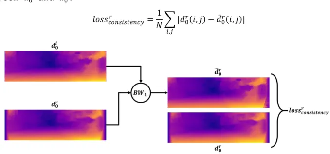
A third loss term is designed to enforce consistency between the two predictions. For this purpose, the left inferred disparity 𝑑₀𝑙

is backward-warped according to the right inferred disparity 𝑑₀𝑟 _,

(15)

indi-15

cate as 𝑑̃₀𝑟_{. The actual loss term is given by the L1 difference}

be-tween 𝑑₀𝑟_{and 𝑑̃} 0𝑟: 𝑙𝑜𝑠𝑠_{𝑐𝑜𝑛𝑠𝑖𝑠𝑡𝑒𝑛𝑐𝑦}𝑟 = 1 𝑁∑ |𝑑0 𝑟_{(𝑖, 𝑗) − 𝑑̃} 0 𝑟_{(𝑖, 𝑗)|} 𝑖,𝑗

Figure 2.7 – A visual description showing the procedure for the computation of left-right consistency loss with respect to the right inferred disparity.

The total loss for each training sample is then given by the combi-nation of all these contributions relative to both predictions and can be expressed as follows:

𝑙𝑜𝑠𝑠 = (𝑙𝑜𝑠𝑠_{𝑖𝑚𝑎𝑔𝑒}𝑙 + 𝑙𝑜𝑠𝑠_{𝑖𝑚𝑎𝑔𝑒}𝑟 ) ⋅ 𝑖𝑚𝑎𝑔𝑒_{𝑤𝑒𝑖𝑔ℎ𝑡}+ (𝑙𝑜𝑠𝑠_{𝑠𝑚𝑜𝑜𝑡ℎ𝑛𝑒𝑠𝑠}𝑙 + 𝑙𝑜𝑠𝑠_{𝑠𝑚𝑜𝑜𝑡ℎ𝑛𝑒𝑠𝑠}𝑟 )

⋅ 𝑠𝑚𝑜𝑜𝑡ℎ𝑛𝑒𝑠𝑠_{𝑤𝑒𝑖𝑔ℎ𝑡}+ (𝑙𝑜𝑠𝑠_{𝑐𝑜𝑛𝑠𝑖𝑠𝑡𝑒𝑛𝑐𝑦}𝑙 + 𝑙𝑜𝑠𝑠_{𝑐𝑜𝑛𝑠𝑖𝑠𝑡𝑒𝑛𝑐𝑦}𝑟 ) ⋅ 𝑐𝑜𝑛𝑠𝑖𝑠𝑡𝑒𝑛𝑐𝑦_{𝑤𝑒𝑖𝑔ℎ𝑡} Weighting coefficients default at 1.0 for image and consistency terms and at 0.1 for the smoothness term.

Figure 2.8 – A diagram showing how both the left and right items in a stereo pair are used for training (only the image loss is shown). Inference only depends on 𝑙₀.

(16)

16

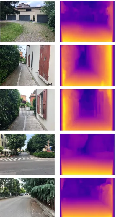
Even though the training procedure requires both the initial left and right images, inference depends on 𝑙₀ alone, while 𝑟₀ is only used for the generation of loss. For this reason, we are not re-quired to provide the right element of the stereo pair if we are just interested in inferring disparity, which makes it possible to obtain these predictions from very simple imaging setups, including generic smartphone cameras. Figure 2.9 shows some examples of depth inferences for images captured using a mobile phone camera.

(17)

17

Figure 2.9 – Images captured from a smartphone and their disparity maps inferred through Monodepth.

(18)

(19)

19

3. Monoflow

Since the purpose of this thesis is producing an unsupervised meth-odology for scene flow inference, it is necessary to devise a pro-cedure for optical flow prediction to work in synergy with Monodepth, thus allowing for the combination of disparity and opti-cal flow information (as already mentioned in chapter 2.2).

Instead of relying on a different neural network model, the choice was made to carry out these predictions through a slightly modified version of Godard et al.’s architecture, repurposed to produce two-dimensional output, that will be referred to as Monoflow.

3.1. Architecture and Training

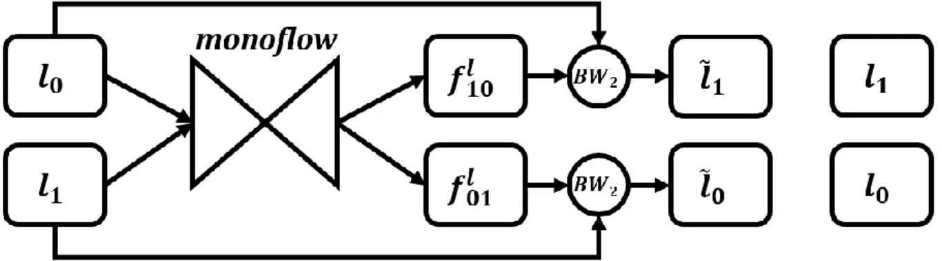
Instead of using a stereo pair, Monoflow is trained on a pair of subsequent monocular frames 𝑙₀ and 𝑙₁. Note that, unlike Monodepth, the new architecture uses both input images for the inference. This does reduce the portability of our solution at prediction-time, as they refer to the same camera and can therefore be assumed to be available on simple capture setups at prediction time.

Figure 3.1 – A diagram showing how two subsequent frames referring to the same camera are used for training Monoflow (only image loss is shown). Inference depends on both 𝑙₀ and 𝑙₁.

The network is still organised in an Encoder/Decoder structure, based on VGG. It must be noticed that, since optical flow conveys information about both horizontal and vertical displacements,

(20)

out-20 put predictions 𝑓₀₁𝑙 _{and 𝑓}

10𝑙 will include two channels each. These two

predictions correspond respectively to the forward flow that ac-counts for how points in 𝑙0 move to their new positions in 𝑙1 and to

the backward flow, expressing how points in 𝑙1 should move to go

back to their positions in 𝑙0. As pixels’ movements may be positive

and negative along each axis (unlike disparity), it is required to produce 𝑓₀₁𝑙 _{and 𝑓}

10𝑙 through convolutional layers whose activation

function is not exclusively positive. For this reason, sigmoidal activations were replaced by hyperbolic tangents in these layers. The loss function used to train Monoflow is made up of three pairs terms (that refer both to the forward and backward flow), corre-sponding to the ones used for Monodepth:

𝑙𝑜𝑠𝑠 = (𝑙𝑜𝑠𝑠_{𝑖𝑚𝑎𝑔𝑒}01 + 𝑙𝑜𝑠𝑠_{𝑖𝑚𝑎𝑔𝑒}10 ) ⋅ 𝑖𝑚𝑎𝑔𝑒_{𝑤𝑒𝑖𝑔ℎ𝑡}+ (𝑙𝑜𝑠𝑠_{𝑠𝑚𝑜𝑜𝑡ℎ𝑛𝑒𝑠𝑠}01 + 𝑙𝑜𝑠𝑠_{𝑠𝑚𝑜𝑜𝑡ℎ𝑛𝑒𝑠𝑠}10 )

⋅ 𝑠𝑚𝑜𝑜𝑡ℎ𝑛𝑒𝑠𝑠_{𝑤𝑒𝑖𝑔ℎ𝑡}+ (𝑙𝑜𝑠𝑠_{𝑐𝑜𝑛𝑠𝑖𝑠𝑡𝑒𝑛𝑐𝑦}01 + 𝑙𝑜𝑠𝑠_{𝑐𝑜𝑛𝑠𝑖𝑠𝑡𝑒𝑛𝑐𝑦}10 ) ⋅ 𝑐𝑜𝑛𝑠𝑖𝑠𝑡𝑒𝑛𝑐𝑦_{𝑤𝑒𝑖𝑔ℎ𝑡}

In the following, we will only describe loss terms relating to backward flow 𝑓₁₀𝑙 _{. The corresponding formulae for forward flow terms}

can be obtained by swapping all occurrences of 0 and 1 in the sym-bols.

The smoothness term applies an L1 penalty on the gradient of the optical flow prediction, weighted by the image gradient to intro-duce tolerance with respect to grayscale image discontinuities (𝑓₁₀𝑙

refers to 𝑙1). Loss terms are initially computed for each optical

flow channel separately and the overall result is given by their average. 𝑙𝑜𝑠𝑠_{𝑠𝑚𝑜𝑜𝑡ℎ𝑛𝑒𝑠𝑠}10 _𝑥 = 1 𝑁∑|𝜕𝑥𝑓10 𝑙 _{(𝑖, 𝑗)} 𝑥|𝑒−‖𝜕𝑥𝑙1(𝑖,𝑗)‖+ |𝜕𝑦𝑓10𝑙 (𝑖, 𝑗)𝑥|𝑒−‖𝜕𝑦𝑙1(𝑖,𝑗)‖ 𝑖,𝑗 𝑙𝑜𝑠𝑠_{𝑠𝑚𝑜𝑜𝑡ℎ𝑛𝑒𝑠𝑠}10 _𝑦 = 1 𝑁∑|𝜕𝑥𝑓10 𝑙 _{(𝑖, 𝑗)} 𝑦|𝑒−‖𝜕𝑥𝑙1(𝑖,𝑗)‖+ |𝜕𝑦𝑓10𝑙 (𝑖, 𝑗)𝑦|𝑒−‖𝜕𝑦𝑙1(𝑖,𝑗)‖ 𝑖,𝑗 𝑙𝑜𝑠𝑠_{𝑠𝑚𝑜𝑜𝑡ℎ𝑛𝑒𝑠𝑠}10 =𝑙𝑜𝑠𝑠𝑠𝑚𝑜𝑜𝑡ℎ𝑛𝑒𝑠𝑠𝑥 10 _{+ 𝑙𝑜𝑠𝑠} 𝑠𝑚𝑜𝑜𝑡ℎ𝑛𝑒𝑠𝑠𝑦 10 2

(21)

21

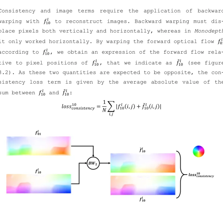
Consistency and image terms require the application of backward warping with 𝑓₁₀𝑙 _{to reconstruct images. Backward warping must}

dis-place pixels both vertically and horizontally, whereas in Monodepth it only worked horizontally. By warping the forward optical flow 𝑓₀₁𝑙

according to 𝑓₁₀𝑙 _{, we obtain an expression of the forward flow}

rela-tive to pixel positions of 𝑓₁₀𝑙 _{, that we indicate as 𝑓̃}

10𝑙 (see figure

3.2). As these two quantities are expected to be opposite, the con-sistency loss term is given by the average absolute value of the sum between 𝑓₁₀𝑙 _{and 𝑓̃}

10𝑙 : 𝑙𝑜𝑠𝑠_{𝑐𝑜𝑛𝑠𝑖𝑠𝑡𝑒𝑛𝑐𝑦}10 = 1 𝑁∑ |𝑓10 𝑙 _{(𝑖, 𝑗) + 𝑓̃} 10𝑙 (𝑖, 𝑗)| 𝑖,𝑗

Figure 3.2 – A visual description showing the procedure for the computation of left-right consistency loss with respect to the right inferred disparity. The correspondence between

colour hue and motion direction can be inferred from the colour wheel.

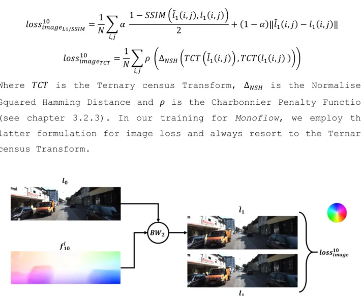
To generate the image loss term used in Monoflow’s training, a com-parison is made between the reconstruction of 𝑙1 that is obtained by

backward-warping 𝑙₀ according to 𝑓₁₀𝑙 _{, that is 𝑙̃}

1, and 𝑙1 itself (see

figure 3.3). In addition to the comparison methodology applied in by Godard et al., combining L1 and SSIM distances, a second dis-tance measure based on Ternary census Transform can also be used as suggested in [23]. Both formulae for the image loss term are listed

(22)

22

in the following; please refer to chapter 3.2 for a detailed expla-nation of the second possibility.

𝑙𝑜𝑠𝑠_{𝑖𝑚𝑎𝑔𝑒}10 _{𝐿1/𝑆𝑆𝐼𝑀} = 1 𝑁∑ 𝛼 1 − 𝑆𝑆𝐼𝑀 (𝑙̃₁(𝑖, 𝑗), 𝑙1(𝑖, 𝑗)) 2 + (1 − 𝛼)‖𝑙̃1(𝑖, 𝑗) − 𝑙1(𝑖, 𝑗)‖ 𝑖,𝑗 𝑙𝑜𝑠𝑠_{𝑖𝑚𝑎𝑔𝑒}10 _𝑇𝐶𝑇 = 1 𝑁∑ 𝜌 (Δ𝑁𝑆𝐻(𝑇𝐶𝑇 (𝑙̃1(𝑖, 𝑗)) , 𝑇𝐶𝑇(𝑙1(𝑖, 𝑗) ))) 𝑖,𝑗

Where 𝑇𝐶𝑇 is the Ternary census Transform, Δ𝑁𝑆𝐻 is the Normalised

Squared Hamming Distance and 𝜌 is the Charbonnier Penalty Function (see chapter 3.2.3). In our training for Monoflow, we employ the latter formulation for image loss and always resort to the Ternary census Transform.

Figure 3.3 – A visual description showing how the second frame is tentatively recon-structed by backward-warping the first frame with backward flow. The discrepancy between

the reconstructed and the original image is the primary source of loss.

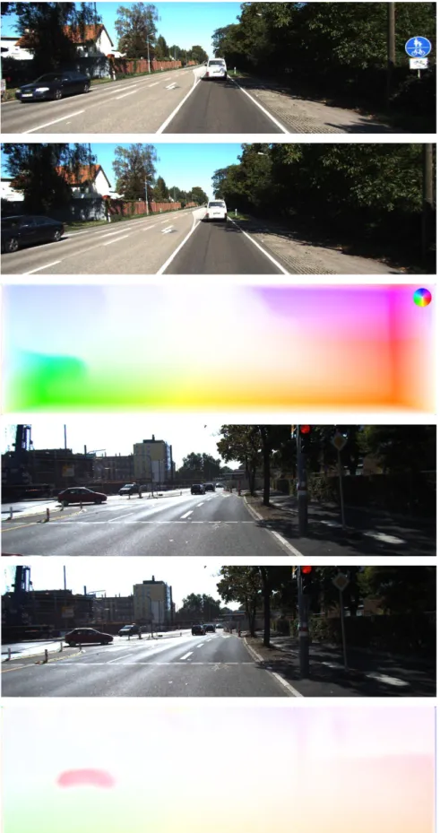
As qualitatively illustrated by the results in figure 3.4, Monoflow appears to be effective at optical flow prediction and requires a training routine that is much simpler than the one of Flownet [5, 22], which is one of the most popular deep-learning architectures for optical flow regression.

(23)

23

Figure 3.4 – Examples of optical flow inferences made by Monoflow on images coming from the KITTI dataset.

(24)

24

3.2. Census Transform

The newly introduced formulation for the image loss term is in-spired by the work of Meister et al. in [23]. It relies on the gen-eration of a descriptor for each pixel in the images to be com-pared, which summarises information about its neighbourhood in a bit string.

3.2.1. Census Transform

The census Transform was first proposed by Zabih and Woodfill in [8] as a non-parametric local transform to tackle the correspond-ence problems by highlighting the relation between intensity values in adjacent pixels.

Let 𝜉 be a binary function of two grey level values, defined as follows:

𝜉(𝑃, 𝑃′_{) = {}0 𝑖𝑓 𝑃 > 𝑃′

1 𝑖𝑓 𝑃 ≤ 𝑃′

Let 𝐼(𝑖, 𝑗) denote the grey level of the pixel at position (𝑖, 𝑗) in im-age 𝐼 , let 𝐷 be a set of displacements that we use to express its neighbourhood, the Census Transform of 𝐼(𝑖, 𝑗) produces a bit string according to the following formula:

𝑅𝜏(𝐼(𝑖, 𝑗)) = ##

𝑘,𝑙∈𝐷𝜉(𝐼(𝑖, 𝑗), 𝐼(𝑖 + 𝑘, 𝑗 + 𝑙))

where ## denotes concatenation. The resulting bit string is as long as the number of displacements contained in 𝐷.

For instance, consider the following 3x3 image region. 127 128 129

126 𝟏𝟐𝟖 129 127 131 129

The census Transform for the central element with respect to its 8-neighbourhood (visited from left to right and from top to bottom) is given by the linearization of the applications of 𝜉 to the cen-tral pixel and each other pixel in the neighbourhood:

(25)

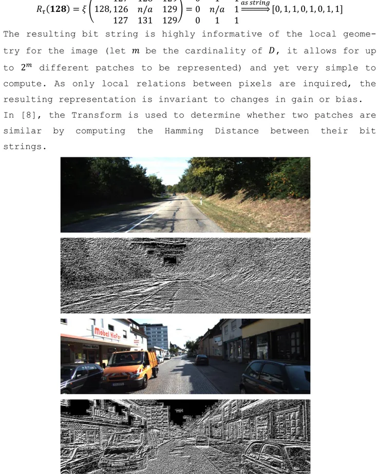
25 𝑅_𝜏(𝟏𝟐𝟖) = 𝜉 (128, 127 128 129 126 𝑛/𝑎 129 127 131 129 ) = 0 1 1 0 𝑛/𝑎 1 0 1 1 𝑎𝑠 𝑠𝑡𝑟𝑖𝑛𝑔 ⇒ [0, 1, 1, 0, 1, 0, 1, 1]

The resulting bit string is highly informative of the local geome-try for the image (let 𝑚 be the cardinality of 𝐷, it allows for up to 2𝑚_{different patches to be represented) and yet very simple to}

compute. As only local relations between pixels are inquired, the resulting representation is invariant to changes in gain or bias. In [8], the Transform is used to determine whether two patches are similar by computing the Hamming Distance between their bit strings.

Figure 3.5 – Examples of the application of the census Transform on KITTI images. The re-sulting bit strings are converted to grey level values (different levels mean different

(26)

26

3.2.2. Ternary census Transform

In [18], Stein modifies the original census Transform proposal by replacing 𝜉 with the following ternary function 𝜉₃ which employs an additional parameter 𝜖 called census:

𝜉₃(𝑃, 𝑃′_{) = {}

−1 𝑖𝑓 𝑃 − 𝑃′> 𝜀 0 𝑖𝑓 |𝑃 − 𝑃′| ≤ 𝜀

1 𝑖𝑓 𝑃′− 𝑃 > 𝜀

The introduction of 𝜀 allows for additional information to be gath-ered, explicitly describing the situation in which the grey levels of 𝑃 and 𝑃′_{are similar. The Ternary census Transform can therefore}

be expressed as:

𝑅_𝜏₃(𝐼(𝑖, 𝑗)) = ##

𝑘,𝑙∈𝐷𝜉3(𝐼(𝑖, 𝑗), 𝐼(𝑖 + 𝑘, 𝑗 + 𝑙))

Note that, while all the advantages that come from the employment of relative intensities between pixels are inherited by the Ternary Transform, the discriminative power of the resulting description string is higher, as we can represent 3𝑚_{different patches.}

The value we choose for census determines how sensitive the trans-form is to noise. For instance, choosing 𝜀 = 0 means that even mini-mal noise alters the descriptions consistently, while 𝜀 = 𝑔𝑟𝑒𝑦_𝑚𝑎𝑥 makes the descriptor insensitive to any kind of intensity varia-tion. Stein recommends choosing 𝜀 = 16 for common 8-bit images. Consider the following example 3x3 image region.

124 74 32 124 𝟔𝟒 18 157 116 84

If we assume that 𝜀 = 16, the Ternary census Transform for the cen-tral element with respect to its 8-neighbourhood (visited from left to right and from top to bottom) is given by:

𝑅_𝜏₃(𝟔𝟒) = 𝜉3(64, 124 74 32 124 𝑛/𝑎 18 157 116 84 ) = 1 0 −1 1 𝑛/𝑎 −1 1 1 1 𝑎𝑠 𝑠𝑡𝑟𝑖𝑛𝑔 ⇒ [1, 0, −1, 1, −1, 1, 1, 1]

(27)

27

With respect to the binary descriptor, storing the ternary string requires encoding the tree values. This means that twice as much computer memory as in the precious case is needed, as the three possible values must be encoded with the following 2-bit combina-tions:

{

−1 = 00 0 = 01 1 = 11

Although more efficient encodings could be devised (e.g. storing the most frequent value with a single bit and the others with two), the one specified above is still preferred as the distance between the two opposite values −1 and 1 is maximised as far as Hamming Distance is concerned.

The descriptor string from the example above could then be encoded in 16 bits as [11, 01, 00, 11, 00, 11, 11, 11].

(28)

28

Figure 3.6 – Examples of the application of the Ternary census Transform on KITTI images. The resulting decoded bit strings are decoded to red and blue level values (different

levels mean different strings).

3.2.3. Computing image loss

As anticipated in chapter 3.1, the Ternary census Transform can be used to compute a loss term accounting for the dissimilarity be-tween an image 𝐼 and its reconstruction 𝐼̃, as described in [23]:

𝑙𝑜𝑠𝑠_{𝑖𝑚𝑎𝑔𝑒}𝐼 _𝑇𝐶𝑇 = 1

𝑁∑ 𝜌 (Δ𝑁𝑆𝐻(𝑇𝐶𝑇 (𝐼̃(𝑖, 𝑗)) , 𝑇𝐶𝑇(𝐼(𝑖, 𝑗) )))

(29)

29

𝐼 and 𝐼̃ are initially elaborated through the Ternary census Trans-form, yielding a descriptive ternary string for each Image pixel. These richer descriptions are pixel-wise compared through the Nor-malised Squared Hamming Distance Δ_𝑁𝑆𝐻(𝑆, 𝑆′_{). Given two strings 𝑆 and}

𝑆′ with length 𝑙, we define this function as:

Δ_𝑁𝑆𝐻(𝑆, 𝑆′_{) = ∑} (𝑆(𝑖) − 𝑆′(𝑖))2

0.1 + (𝑆(𝑖) − 𝑆′(𝑖))2 𝑙

𝑖=1

where 𝐻𝐷 denotes simple Hamming Distance. As can be clearly seen in figure 3.7, employing Δ_𝑁𝑆𝐻 means introducing a huge penalty even in the case of small differences between the strings. This is fur-ther exemplified in figure 3.8, in which a visual comparison be-tween the Hamming distance and Δ_𝑁𝑆𝐻 of two images is shown.

Figure 3.7 – Graph showing how 𝛥𝑁𝑆𝐻’s output relates to the Hamming Distance for a single

string item. The comparison made by 𝛥𝑁𝑆𝐻 is normalised between 0 and 1 and even small edit

(30)

30 (a)

(b)

(c)

(d)

Figure 3.8 – An image from the KITTI dataset (a), its reconstruction with Monoflow (b) and a visual comparison between their Hamming Distance (c) and their Normalised Squared

Hamming Distance (d).

The result of Δ_𝑁𝑆𝐻 is further elaborated through the robust Gener-alised Charbonnier Penalty Function 𝜌 as described in [19] with:

𝜌(𝑥) = (𝑥2 + 𝜀2)𝑎

where 𝑎 = 0.45 and 𝜀 small (in our code 𝜀 = 0.001). This function is a differentiable variant of the absolute value, as shown clearly in figure 3.9.

(31)

31

Figure 3.9 – Graph for the Generalised Charbonnier Penalty Function, including a fine zoom to highlight differentiability.

(32)

(33)

33

4. Pantaflow

4.1. Scene flow inference methods

While in chapter 3 we described the necessary modifications that were carried out on the initial Monodepth architecture to come up with a system for optical flow prediction, the present chapter deals with the definition of an unsupervised architecture for scene flow inference referred to as Pantaflow.

To understand the 3D motion of a scene point in space, we need to combine the information we have on its movement along the image plane (optical flow) with information on its translation along the orthogonal axis, which can be expressed as disparity change.

Given two consecutive frames 𝑙0 and 𝑙1, showing an object that moves

in space, we can use Monodepth to infer the two corresponding dis-parity maps 𝑑₀𝑙 _{and 𝑑}

1𝑙. The difference between the disparity value

that we observe for the same moving object in these maps allows us to determine how it moved along the orthogonal axis with respect to the camera plane. As the movement, however, also occurs along image plane, in order to make the two disparity maps easily comparable, one needs to be backward warped with optical flow (that can be in-ferred by Monoflow) so as to compensate movement along the image plane and obtain two “superimposable” maps that can be easily com-pared by the means of a simple difference.

With reference to the visual exemplification of this procedure in figure 4.1, the version of 𝑑₁𝑙_{that is warped to be made comparable}

with 𝑑₀𝑙_{is called 𝑟}

0𝑑1𝑙. By inverting the two disparity maps and

us-ing the opposite optical flow for warpus-ing, we can similarly obtain 𝑟₁𝑑₀𝑙. We will refer to 𝑟₀𝑑₁𝑙 and 𝑟₁𝑑₀𝑙 as relative disparity maps.

(34)

34 (a) (b) (c) (d) (e) (f) (g) (h)

Figure 4.1 – Visual description of how disparity change can be used to assess depth flow: (a) 3D rendering of the simple scene, with some scene flow vectors and camera position; (b) 𝑙0; (c) 𝑑0𝑙; (d) 𝑙1; (e) 𝑑1𝑙; (f) 𝑓01𝑙 : optical flow map relative to 𝑙0; (g) 𝑟0𝑑1𝑙:

reprojec-tion of 𝑑₁𝑙_{by using 𝑓}

01𝑙 (backwards); (h) disparity change map given by the difference

be-tween 𝑑₀𝑙_{and 𝑟} 0𝑑1𝑙.

(35)

35

4.2. Architectural hypotheses

Depending on the methodology that we use for predicting relative disparities, we distinguish between two architectures for Panta-flow: mono* (mono-star) infers them by warping Monodepth’s predic-tions with Monoflow’s, while unison regresses them directly.

(a) (b)

Figure 4.2 – Visual comparison of the structures of the two candidate architectures for Pantaflow: mono* (a) and unison (b).

4.2.1. Mono*

The first proposed architecture for Pantaflow (see figure 4.2a) is called mono* and consists of the juxtaposition of a Monodepth-like encoder/decoder-structured CNN and a separate Monoflow-like encod-er/decoder-structured CNN, whose combined predictions we estab-lished to be sufficient to express scene flow. In order to obtain the two relative disparity maps, the portion of the net that infers depth is initially used to predict disparities for both input frames 𝑙₀ and 𝑙₁. The optical flow information that is regressed by the other sub-network is then used to re-project 𝑑₀𝑙_{and 𝑑}

1𝑙 so as to

localise their values to the position of the corresponding points at time 1 and 0 respectively, yielding 𝑟1𝑑0𝑙 and 𝑟0𝑑1𝑙.

(36)

36

Loss gradient is computed at training time from 𝑑₀𝑙_{, 𝑑}

0𝑟, 𝑓10𝑙 and 𝑓01𝑙

predictions exactly as in Monodepth and Monoflow. Coherently, rela-tive disparity maps predicted at four decreasing scales and are al-so used as a al-source of loss by the means of a weighted sum between an image loss term, a smoothness loss term and a consistency loss term, as described in section 4.3.

4.2.2. Unison

The second architecture that we propose for Pantaflow (figure 4.2b), called unison, relies on a simplified organisation by fac-torising the encoders between the two encoder/decoder-structures that we presented in mono*. Temporal pairs of input frames are fed into a single encoder that is then connected to three distinct de-coders, in charge of inferring disparity, optical flow and relative disparity respectively. This means that 𝑟1𝑑0𝑙 and 𝑟0𝑑1𝑙 are not

ob-tained through warping, but directly as products from one of the decoders. These predictions are logically employed to generate loss gradient along with the inferences coming from the other two decod-ers, as described in section 4.3.

4.3. Training Pantaflow

Regardless of the specific Pantaflow architecture employed, the network is trained by generating loss terms from the predicted dis-parity maps at time 0 𝑑₀𝑙 _{and 𝑑}

0

𝑟_{, from the inferred optical flow}

maps 𝑓₁₀𝑙 _{and 𝑓}

01𝑙 and from the two relative left disparity maps 𝑟0𝑑1𝑙

and 𝑟₁𝑑₀𝑙. These contributions are simply added up to form the over-all training loss, after dividing by two the term that relates to optical flow. This is done in order to enforce balance among the terms, as 𝑓₁₀𝑙 _{and 𝑓}

01𝑙 have twice as many channels as the other maps

and therefore generate twice as much loss gradient.

𝑙𝑜𝑠𝑠_{𝑝𝑎𝑛𝑡𝑎𝑓𝑙𝑜𝑤} = 𝑙𝑜𝑠𝑠_{𝑑𝑖𝑠𝑝}+ 𝑙𝑜𝑠𝑠_{𝑟𝑒𝑙𝑑𝑖𝑠𝑝}+𝑙𝑜𝑠𝑠𝑜𝑝𝑡𝑓𝑙𝑜𝑤 2

(37)

37

𝑙𝑜𝑠𝑠𝑑𝑖𝑠𝑝 and 𝑙𝑜𝑠𝑠𝑜𝑝𝑡𝑓𝑙𝑜𝑤 are computed like the overall losses for

Monodepth and Monoflow respectively:

𝑙𝑜𝑠𝑠𝑑𝑖𝑠𝑝 = (𝑙𝑜𝑠𝑠𝑖𝑚𝑎𝑔𝑒𝑙 + 𝑙𝑜𝑠𝑠𝑖𝑚𝑎𝑔𝑒𝑟 ) ⋅ 𝑖𝑚𝑎𝑔𝑒𝑤𝑒𝑖𝑔ℎ𝑡+ (𝑙𝑜𝑠𝑠𝑠𝑚𝑜𝑜𝑡ℎ𝑛𝑒𝑠𝑠𝑙 + 𝑙𝑜𝑠𝑠𝑠𝑚𝑜𝑜𝑡ℎ𝑛𝑒𝑠𝑠𝑟 )

⋅ 𝑠𝑚𝑜𝑜𝑡ℎ𝑛𝑒𝑠𝑠𝑤𝑒𝑖𝑔ℎ𝑡+ (𝑙𝑜𝑠𝑠𝑐𝑜𝑛𝑠𝑖𝑠𝑡𝑒𝑛𝑐𝑦𝑙 + 𝑙𝑜𝑠𝑠𝑐𝑜𝑛𝑠𝑖𝑠𝑡𝑒𝑛𝑐𝑦𝑟 ) ⋅ 𝑐𝑜𝑛𝑠𝑖𝑠𝑡𝑒𝑛𝑐𝑦𝑤𝑒𝑖𝑔ℎ𝑡

𝑙𝑜𝑠𝑠_{𝑜𝑝𝑡𝑓𝑙𝑜𝑤} = (𝑙𝑜𝑠𝑠_{𝑖𝑚𝑎𝑔𝑒}01 + 𝑙𝑜𝑠𝑠_{𝑖𝑚𝑎𝑔𝑒}10 ) ⋅ 𝑖𝑚𝑎𝑔𝑒_{𝑤𝑒𝑖𝑔ℎ𝑡}+ (𝑙𝑜𝑠𝑠_{𝑠𝑚𝑜𝑜𝑡ℎ𝑛𝑒𝑠𝑠}01 + 𝑙𝑜𝑠𝑠_{𝑠𝑚𝑜𝑜𝑡ℎ𝑛𝑒𝑠𝑠}10 ) ⋅ 𝑠𝑚𝑜𝑜𝑡ℎ𝑛𝑒𝑠𝑠_{𝑤𝑒𝑖𝑔ℎ𝑡}+ (𝑙𝑜𝑠𝑠_{𝑐𝑜𝑛𝑠𝑖𝑠𝑡𝑒𝑛𝑐𝑦}01 + 𝑙𝑜𝑠𝑠_{𝑐𝑜𝑛𝑠𝑖𝑠𝑡𝑒𝑛𝑐𝑦}10 ) ⋅ 𝑐𝑜𝑛𝑠𝑖𝑠𝑡𝑒𝑛𝑐𝑦_{𝑤𝑒𝑖𝑔ℎ𝑡}

Where the particular loss terms are the ones defined in chapters 2.3.2 and 3.1.

The contribution to loss coming from relative disparities is simi-larly computed as

𝑙𝑜𝑠𝑠_{𝑟𝑒𝑙𝑑𝑖𝑠𝑝} = (𝑙𝑜𝑠𝑠_{𝑖𝑚𝑎𝑔𝑒}𝑟𝑒𝑙0 + 𝑙𝑜𝑠𝑠_{𝑖𝑚𝑎𝑔𝑒}𝑟𝑒𝑙1 ) ⋅ 𝑖𝑚𝑎𝑔𝑒_{𝑤𝑒𝑖𝑔ℎ𝑡}+ (𝑙𝑜𝑠𝑠_{𝑠𝑚𝑜𝑜𝑡ℎ𝑛𝑒𝑠𝑠}𝑟𝑒𝑙0 + 𝑙𝑜𝑠𝑠_{𝑠𝑚𝑜𝑜𝑡ℎ𝑛𝑒𝑠𝑠}𝑟𝑒𝑙1 ) ⋅ 𝑠𝑚𝑜𝑜𝑡ℎ𝑛𝑒𝑠𝑠_{𝑤𝑒𝑖𝑔ℎ𝑡}+ (𝑙𝑜𝑠𝑠_{𝑐𝑜𝑛𝑠𝑖𝑠𝑡𝑒𝑛𝑐𝑦}𝑟𝑒𝑙0 + 𝑙𝑜𝑠𝑠_{𝑐𝑜𝑛𝑠𝑖𝑠𝑡𝑒𝑛𝑐𝑦}𝑟𝑒𝑙1 ) ⋅ 𝑐𝑜𝑛𝑠𝑖𝑠𝑡𝑒𝑛𝑐𝑦_{𝑤𝑒𝑖𝑔ℎ𝑡}

While disparities and relative disparities are very similar in that they are both always positive and ultimately express the same quan-tity, a novel warping procedure needs to be defined in order to use relative disparities in reprojections when we compute the image loss term. In the following, we will only examine the way we use 𝑟₀𝑑₁𝑙 to produce image loss. The equivalent contribution for 𝑟₁𝑑₀𝑙 is obtained by inverting all 0 and 1 indices in the formulae that will be introduced.

Since 𝑟₀𝑑₁𝑙 is a backward flow-warped version of the left disparity at time 1 𝑑₁𝑙_{, it can be used to tentatively reconstruct 𝑙}

1 by

back-ward-warping 𝑟₁, in analogy with what Monodepth does. In order to do this, however, it is necessary to refer 𝑟₀𝑑₁𝑙 to time 1 by the

(38)

38

means of a backward warping with flow 𝑓₁₀𝑙 _{. The result of this}

warp-ing is expressed as 𝑑̃₁𝑙_{in figure 4.2 and can be used to warp 𝑟} 1,

thus obtaining 𝑙̃̃₁, which is compared with 𝑙₁ by the means of the combination of L1 and SSIM distance metrics that we already pre-sented in chapter 3, as expressed in the formula that follows:

𝑙𝑜𝑠𝑠_{𝑖𝑚𝑎𝑔𝑒}𝑟𝑒𝑙0 = 1 𝑁∑ 𝛼

1 − 𝑆𝑆𝐼𝑀 (𝑙̃̃₁(𝑖, 𝑗), 𝑙1(𝑖, 𝑗))

2 + (1 − 𝛼)‖𝑙̃̃1(𝑖, 𝑗) − 𝑙1(𝑖, 𝑗)‖

𝑖,𝑗

Figure 4.2 – A visual description showing how the second left frame is tentatively recon-structed by backward-warping the second right frame with warped relative disparity. The

difference between reconstructed and original images is the primary source of loss.

For the term that enforces consistency between couples of predic-tions, we simply choose to compare 𝑑̃₁𝑙_{as obtained above with the}

other relative disparity.

𝑙𝑜𝑠𝑠_{𝑐𝑜𝑛𝑠𝑖𝑠𝑡𝑒𝑛𝑐𝑦}𝑟𝑒𝑙0 = 1

𝑁∑ |𝑟1𝑑0

𝑙_{(𝑖, 𝑗) − 𝑑̃} 1𝑙(𝑖, 𝑗)| 𝑖,𝑗

(39)

39

Figure 4.3 – A visual description showing the procedure for the computation of consisten-cy loss. Notice that this is a simple one-step warping with optical flow.

Finally, the smoothness term is computed like in the previous net-works, by associating a penalty to high 𝑟₀𝑑₁𝑙 gradients which is weighted accordingly to image gradients to introduce tolerance over image discontinuities. Notice how the image we use is 𝑙₀, as 𝑟₀𝑑₁𝑙 is expected to refer to it.

𝑙𝑜𝑠𝑠_{𝑠𝑚𝑜𝑜𝑡ℎ𝑛𝑒𝑠𝑠}𝑟𝑒𝑙0 = 1

𝑁∑|𝜕𝑥𝑟0𝑑1

𝑙_{(𝑖, 𝑗)|𝑒}−‖𝜕𝑥𝑙0(𝑖,𝑗)‖_{+ |𝜕}

𝑦𝑟0𝑑1𝑙(𝑖, 𝑗)|𝑒−‖𝜕𝑦𝑙1(𝑖,𝑗)‖ 𝑖,𝑗

(40)

40

Figure 4.4 – A diagram showing how two subsequent frames referring to the same camera are used for training Pantaflow (only image loss terms are displayed). The network is shown as a black-box as there are no differences in training tied to the specific architecture.

(41)

41

5. Experimental Results

5.1. Training specifications

Training for Pantaflow is carried out on the KITTI dataset [4], re-organised in 28969 temporal pairs of stereo frames. Batches of 8 items are used for each iteration for a grand total of 181100 iter-ations, corresponding to 50 epochs approximately.

An NVIDIA Titan X Graphic Processor equipped with 12 GB of RAM was used for both training and testing.

5.2. Post-Processing

An additional post-processing step similar to the one carried out by Godard et al. in [3] is applied to disparity, optical flow and relative disparity predictions by Pantaflow. Each prediction is separately computed both for the input temporal pair 𝑙₀, 𝑙₁ and its flipped version 𝑙₀𝑓𝑙𝑖𝑝, 𝑙₁𝑓𝑙𝑖𝑝. Let 𝑝 be the resulting prediction that re-lates to the former pair, 𝑝𝑓𝑙𝑖𝑝_{be the one relating to the latter}

pair and 𝑝𝑎𝑣𝑔_{be their average, they are combined as follows (see}

figure 5.1):

• The leftmost 5% of the post-processed result is sampled from 𝑝.

• The rightmost 5% of the post-processed result is sampled from 𝑝𝑓𝑙𝑖𝑝.

• The remaining is sampled from 𝑝𝑎𝑣𝑔

(42)

42

5.3. Results and Comparisons

This section contains a quantitative evaluation of the test of Pan-taflow on the 2015 extension to the KITTI dataset [13]. This da-taset is used as a reference as it comprehensively includes ground truth data for disparity, optical flow and scene flow. Results for these three types of inference are presented separately comparing the two architectures for the proposed network. Where suitable, ad-ditional comparisons will be made with other existing studies.

5.3.1. Disparity Inference

To quantify Pantaflow’s performances as regards disparity map re-gression, we employ the same evaluation code provided by Godard et al. in [3] and we compare our results directly with the one pre-sented in their paper.

The following evaluation metrics are used:

• Absolute Relative Difference (Abs Rel): the absolute mismatch between a ground truth value 𝑣 and its prediction 𝑣̃ , divided by 𝑣 in order to further penalise errors when attempting to predict higher values. This is averaged out by dividing by the total number of pixels 𝑁.

1 𝑁∑

|𝑣𝑖,𝑗− 𝑣̃𝑖,𝑗|

𝑣_𝑖,𝑗

𝑖,𝑗

• Squared Relative Difference (Sq Rel): similar to the one above, squaring the difference between 𝑣 and 𝑣̃.

1 𝑁∑

(𝑣_𝑖,𝑗− 𝑣̃_𝑖,𝑗)2 𝑣_𝑖,𝑗

(43)

43

• Root Mean Squared Error (RMSE): the square root of the average of the squared mismatches between 𝑣 and 𝑣̃.

√_𝑁1∑(𝑣𝑖,𝑗− 𝑣̃𝑖,𝑗) 2

𝑖,𝑗

• Logarithmic Root Mean Squared Error (RMSE log): the one above, where predictions are compared after applying logarithmic function. As log 𝑣 − log 𝑣̃ = log𝑣

𝑣̃ , this metric is much more

sensi-tive to larger differences.

√_𝑁1∑(log 𝑣𝑖,𝑗− log 𝑣̃𝑖,𝑗) 2

𝑖,𝑗

• Outliers percentage: a metric computing the percentage of out-liers, meaning points for which the mismatch between the ground truth value 𝑣 and the predicted value 𝑣̃ exceeds a given absolute threshold 𝑡_𝑎 and the ratio between the mismatch and the ground truth value exceeds a given relative threshold 𝑡_𝑟. In the following, we assume 𝑡_𝑎 = 3.0 and 𝑡_𝑟 = 0.05 for the Abso-lute and Relative Outlier percentage (AROP, also known as

D1-all) and 𝑡_𝑎 = 3.0 and 𝑡_𝑟 = 0 for the Absolute Outliers Percentage (AOP), which expresses this metric disregarding the relative threshold). 1 𝑁∑ 𝛾𝑖,𝑗 𝑖,𝑗 , 𝑤ℎ𝑒𝑟𝑒 𝛾_𝑖,𝑗 = {1 𝑖𝑓 |𝑣𝑖,𝑗− 𝑣̃𝑖,𝑗| ≥ 𝑡𝑎 𝑎𝑛𝑑 |𝑣_𝑖,𝑗− 𝑣̃_𝑖,𝑗| 𝑣̃_𝑖,𝑗 ≥ 𝑡𝑟 0

• Thresholded errors (𝜹 < 𝒕): the percentage of predictions such that their relative size with respect to ground truth (ex-pressed by the maximum between 𝑣

𝑣̃ and 𝑣̃

𝑣 ) is lower than a

(44)

44 1 𝑁∑ 𝛿𝑖,𝑗 𝑖,𝑗 , 𝑤ℎ𝑒𝑟𝑒 𝛿_𝑖,𝑗 = {1 𝑖𝑓 max ( 𝑣_𝑖,𝑗 𝑣̃𝑖,𝑗 ,𝑣̃𝑖,𝑗 𝑣𝑖,𝑗 ) < 𝑡 0 𝑒𝑙𝑠𝑒

The results that are presented in table 5.1 confirm that Pantaflow-mono* outperforms Monodepth with respect to almost every metric, indicating that taking into account optical flow and scene flow in-formation during training allows for a slight, yet consistent, im-provement. Note that this comparison cannot take post-processing into account, as [3] only provides post-processed data for models trained on the KITTI dataset [4] and the Cityscapes dataset [20], while Pantaflow is only trained on the former.

Additionally, it is shown that mono* steadily obtains better scores than unison.

Method Abs Rel Sq Rel RMSE RMSE log AROP 𝛿 < 1.25 𝛿 < 1.252 _{𝛿 < 1.25}3

Monodepth 0.124 1.388 6.125 0.217 0.303 0.841 0.936 0.975 unison 0.153 2.097 7.016 0.253 0.377 0.793 0.911 0.963 mono* 0.122 1.347 6.172 0.215 0.310 0.843 0.937 0.975 unison pp 0.147 1.905 6.709 0.243 0.376 0.796 0.915 0.966 mono* pp 0.116 1.160 5.845 0.206 0.305 0.846 0.943 0.978

Lower is better Higher is better

Table 5.1 – Quantitative evaluation of Pantaflow and Monodepth for disparity inference on the 2015 extension to the KITTI dataset.

(45)

45

Figure 5.2 – Qualitative comparison for disparity maps as predicted by mono*, unison and Monodepth.

5.3.2. Optical Flow Inference

As far as optical flow inference is concerned, we draw a comparison between Pantaflow and Monoflow in terms of the aforementioned Abso-lute Outlier Percentage and on the Average Endpoint Error (EPE). Notice that, since flow is a two-dimensional quantity, the mismatch between the ground truth value 𝑣 = (𝑣𝑥_{, 𝑣}𝑦_{) and predicted value 𝑣̃ =}

(𝑣̃𝑥_{, 𝑣̃}𝑦_{) is computed by the means of the Euclidean distance.}

𝐸𝑃𝐸(𝑣, 𝑣̃) = 1 𝑁∑ √(𝑣𝑖,𝑗 𝑥 _{− 𝑣̃} 𝑖,𝑗𝑥) 2 + (𝑣_𝑖,𝑗𝑦 − 𝑣̃_𝑖,𝑗𝑦)2 𝑖,𝑗 𝐴𝑂𝑃(𝑣, 𝑣̃) = 1 𝑁∑ 𝛾𝑖,𝑗 𝑖,𝑗 , 𝑤ℎ𝑒𝑟𝑒 𝛾_𝑖,𝑗 = {1 𝑖𝑓 √(𝑣𝑖,𝑗𝑥 − 𝑣̃𝑖,𝑗𝑥) 2 + (𝑣_𝑖,𝑗𝑦 − 𝑣̃_𝑖,𝑗𝑦)2 ≥ 3.0 0

The results that can be found in table 5.2 confirm that Pantaflow outperforms Monoflow. This suggests that tackling disparity, rela-tive disparity and optical flow prediction within the same end-to-end training allows for the obtainment of better results. It must be noted that mono* outperforms unison in this task as well.

(46)

46

Method

Occluded Non-occluded

Epe AOP Epe AOP

Monoflow 24.057 0.680 18.017 0.632 unison 22.220 0.638 14.860 0.581 mono* 19.685 0.510 11.988 0.434 Monoflow pp 23.084 0.688 16.909 0.640 unison pp 21.476 0.631 14.679 0.574 mono* pp 18.686 0.506 11.453 0.430

Table 5.2 – Quantitative evaluation of Pantaflow and Monoflow for optical flow prediction on the 2015 extension to the KITTI dataset.

mono* unison Monoflow

Figure 5.3 – Qualitative comparison for optical flow predictions by mono*, unison and Monoflow.

(47)

47

5.3.3. Scene Flow Inference

To account for the performances of the network with respect to sce-ne flow, we firstly evaluate how good it is at predicting relative disparity. This can be quantified by computing the same evaluation metrics used for disparity by taking 𝑟₀𝑑₁𝑙 into account. The results are listed in table 5.3.

Although there are not suitable architectures available for a com-parison in literature, it is once again confirmed that mono* proves to be more effective than unison. In figure 5.4, we show a qualita-tive comparison between relaqualita-tive disparities 𝑟0𝑑1𝑙 predicted by the

two architectures.

Method Abs Rel Sq Rel RMSE RMSE log AROP 𝛿 < 1.25 𝛿 < 1.252 _{𝛿 < 1.25}3

unison 0.238 2.633 7.621 0.299 0.624 0.633 0.900 0.957 mono* 0.234 2.255 7.102 0.287 0.589 0.641 0.909 0.962 unison pp 0.227 2.256 7.272 0.287 0.614 0.645 0.907 0.961 mono* pp 0.223 1.911 6.653 0.274 0.580 0.650 0.916 0.968

Table 5.3 – Quantitative evaluation of Pantaflow’s architectures for relative disparity inference on the 2015 extension to the KITTI dataset.

(48)

48

Figure 5.4 – Qualitative comparison between 𝑟0𝑑1𝑙 quantities as predicted by mono* and

unison.

Figure 5.5 contains a visualisation of the difference between dis-parities at time 0 𝑑₀𝑙_{and their relative equivalent at time 1 𝑟}

0𝑑1𝑙,

which is called disparity change and expresses points’ movements along the orthogonal axis to the image plane.

(49)

49

Figure 5.5 – Qualitative comparison between disparity changes as predicted by mono* and unison.

As it is desirable to have an overall performance index on scene flow inference, we calculate a scene flow Absolute Outlier Percent-age by regarding as outlier any pixel that exceeds the fixed AOP threshold with respect to disparity, relative disparity or optical flow.

The results, which are listed in table 5.4, can be compared against the competitors in the KITTI 2015 scene flow benchmark competition [24], although it must be noted that no disclosed competitor makes use of unsupervised monocular prediction techniques.

Method d0-AOP (D1-all) r0d1-AOP (D2-all) f-AOP (Fl-all) sf-AOP (SF-ALL) unison 0.386 0.622 0.581 0.676 mono* 0.317 0.586 0.434 0.541 unison pp 0.386 0.612 0.574 0.672 mono* pp 0.313 0.576 0.430 0.536

Table 5.4 – Quantitative evaluation of Pantaflow’s architectures in terms of percentage outliers for separate and joint prediction of disparity, relative disparity and optical

(50)

(51)

51

6. Conclusions and Future Developments

In this thesis, a novel neural network model capable of performing unsupervised monocular scene flow prediction was developed. To the best of the author’s knowledge, no published attempt has been made to predict this quantity without supervision by the means of an end-to-end trained model and the broad majority of the existing state-of-the-art techniques have ostensibly longer execution times. The improvement we obtain with respect to [3] confirms that dispar-ity map inference benefits from being tackled side-by-side with op-tical flow and relative disparity prediction.

While availability of Pantaflow represents a meaningful step to-wards the achievement of real-time scene flow prediction, possibly leading to important improvements in many applicative areas, there is definitely room for the attainment of better results via archi-tectural improvements and finer tuning as follows:

• Alternative architectures like FlowNet, that have already proved successful for inferring optical flow, might be de-ployed and trained along with MonoDepth to predict scene flow. • Experimentations can be made by considering different

combina-tions of image difference funccombina-tions in training (e.g. using Census for all image losses).

• According to very recent studies [25], self-supervised train-ing of Encoder/Decoder-structured CNNs might benefit from the loss function being computed for images at full-scale. Tests could be made by up-sampling the predictions that we extract from the deeper layers of the decoder prior to comparing them with the ground truth.

(52)

(53)

53

7. References

[1] S. Vedula, S. Baker, P. Rander, R. Collins and T. Kanade. Three-dimensional scene flow. In Proceedings of the Seventh IEEE International Conference on Computer Vision, volume 2, pages 722–729, 1999.

[2] F. Huguet and F. Devernay. A variational method for scene flow estimation from stereo sequences. In Computer Vision, 2007. ICCV 2007. IEEE 11th International Conference on, pages 1–7. IEEE, 2007.

[3] C. Godard, O. Mac Aodha and G. J. Brostow. Unsupervised monoc-ular depth estimation with left-right consistency. In Computer Vision and Pattern Recognition, 2017.

[4] A. Geiger, P. Lenz and R. Urtasun. Are we ready for autonomous driving? The kitti vision benchmark suite. In Conference on Computer Vision and Pattern Recognition (CVPR), 2012.

[5] A. Dosovitskiy, P. Fischer, E. Ilg, P. Hausser, C. Hazirbas, V. Golkov, P. van der Smagt, D. Cremers and T. Brox. Flownet: Learning optical flow with convolutional networks. In the IEEE International Conference on Computer Vision (ICCV), December 2015.

[6] H. Zhao, O. Gallo, I. Frosio and J.Kautz. Loss Functions for Neural Networks for Image Processing. ArXiv e-prints, Nov. 2015.

(54)

54

[7] C. Vogel, K. Schindler and S. Roth. 3d scene flow estimation with a piece-wise rigid scene model. International Journal of Computer Vision, 115(1):1–28, 2015.

[8] R. Zabih and J. Woodfill. Non-parametric local transforms for computing visual correspondence. In ECCV 1994.

[9] J. Flynn, I. Neulander, J. Philbin and N. Snavely. Deepstereo: Learning to predict new views from the world’s imagery. In CVPR, 2016.

[10] J. Zbontar and Y. LeCun. Computing the stereo matching cost with a convolutional neural network. In Conference on Computer Vision and Pattern Recognition (CVPR), 2015.

[11] N. Mayer, E. Ilg, P. Häusser, P. Fischer, D. Cremers, A. Doso-vitskiy and T. Brox. A large dataset to train convolutional networks for disparity, optical flow, and scene flow estima-tion. In the IEEE Conference on Computer Vision and Pattern Recognition (CVPR), 2016.

[12] T. Taniai, S. N. Sinha and Y. Sato. Fast multi-frame stereo scene flow with motion segmentation. In the IEEE Conference on Computer Vision and Pattern Recognition (CVPR), July 2017.

[13] M. Menze and A. Geiger. Object scene flow for autonomous vehi-cles. In Conference on Computer Vision and Pattern Recognition (CVPR), 2015.

[14] M. Poggi and S. Mattoccia. Learning to predict stereo relia-bility enforcing local consistency of confidence maps. IEEE Conference on Computer Vision and Pattern Recognition (CVPR 2017), Jul. 2017.

(55)

55

[15] A. Tonioni, M. Poggi, L. Di Stefano and S. Mattoccia. Unsuper-vised Adaptation for Deep Stereo. IEEE International Confer-ence on Computer Vision (ICCV 2017), Oct. 2017.

[16] M. Bai, W. Luo, K. Kundu and R. Urtasun. Exploiting semantic information and deep matching for optical flow. In European Conference on Computer Vision, pages 154–170. Springer, 2016.

[17] A. Behl, O. H. Jafari, S. K. Mustikovela, H. A. Alhaija, C. Rother and A. Geiger. Bounding boxes, segmentations and object coordinates: How important is recognition for 3d scene flow estimation in autonomous driving scenarios? In International Conference on Computer Vision (ICCV), 2017.

[18] F. Stein. Efficient computation of optical flow using the cen-sus transform. In DAGM 2004.

[19] D. Sun, S. Roth and M. J. Black. A Quantitative Analysis of Current Practices in Optical Flow Estimation and the Princi-ples Behind Them. In the International Journal of Computer Vi-sion, Volume 106, pp. 115-137. Jan. 2014.

[20] M. Cordts, M. Omran, S. Ramos, T. Rehfeld, M. Enzweiler, R. Benenson, U. Franke, S. Roth and B. Schiele. The cityscapes dataset for semantic urban scene understanding. In CVPR, 2016.

[21] Y. Wang, Y. Yang, Z. Yang, L. Zhao, P. Wang and W. Xu. Occlu-sion Aware Unsupervised Learning of Optical Flow. ArXiv e-prints, Nov. 2017.

[22] E. Ilg, N. Mayer, T. Saikia, M. Keuper, A. Dosovitskiy and T. Brox. FlowNet 2.0: Evolution of Optical Flow Estimation with

(56)

56

Deep Networks. In IEEE Conference on Computer Vision and Pat-tern Recognition (CVPR), Jul. 2017.

[23] S. Meister, J. Hur and S. Roth. UnFlow: Unsupervised Learning of Optical Flow with a Bidirectional Census Loss, in AAAI, Feb. 2018

[24] The benchmark refers to [13] and can be found at http://www.cvlibs.net/datasets/kitti/eval_scene_flow.php.

[25] C. Godard, O. M. Aodha, G. J. Brostow. Digging into self-supervised monocular depth estimation. ArXiv e-prints, Jun. 2018.

[26] Xie, R. Girshick and A. Farhadi. Deep3d: Fully automatic 2d-to-3d video conversion with deep convolutional neural net-works. In ECCV, 2016.

[27] M. Poggi, F. Aleotti, F. Tosi, S. Mattoccia. Towards real-time unsupervised monocular depth estimation on CPU. Accepted at IEEE/RSJ International Conference on Intelligent Robots and Systems (IROS 2018), Madrid, Spain, October, 1-5, 2018.