Automatic chord recognition based on the probabilistic modeling of diatonic modal harmony

(1)

POLITECNICO DI MILANO Facoltà di Ingegneria dell’Informazione Corso di Laurea in Ingegneria e Design del suono

Dipartimento di Elettronica e Informazione

Automatic chord recognition based on the

probabilistic modeling of diatonic modal

harmony

Supervisor: Prof. Augusto Sarti

Assistant supervisor: Dr. Massimiliano Zanoni

Master graduation thesis by: Bruno Di Giorgi, ID 740696

(2)

(3)

POLITECNICO DI MILANO Facoltà di Ingegneria dell’Informazione Corso di Laurea in Ingegneria e Design del suono

Dipartimento di Elettronica e Informazione

Riconoscimento automatico di accordi

basato sul modello probabilistico

dell’armonia modale diatonica

Relatore: Prof. Augusto Sarti

Correlatore: Dr. Massimiliano Zanoni

Tesi di Laurea di: Bruno Di Giorgi, matricola 740696

(4)

(5)

Abstract

One of the distinctive traits of our society in the last decade is the avail-ability and consequent fruition of multimedia content in digital format. The Internet, the growing density of storage systems and the increasing quality of compressed file formats, played the main roles in this revolution. Nowadays, audio and video contents are easily created, stored and shared by million of people.

This huge amount of data has to be efficiently organized and archived, to ease the fruition of large databases as online shops (as Amazon, iTunes) and content sharing website (Youtube, Soundcloud). The task of extraction of meaningful descriptors from digital audio and classification of musical con-tent are addressed by a new research field named Music Information Retrieval (MIR). Among the descriptors that MIR aims at extracting from audio are rhythm, harmony, melody. These descriptors are meaningful for a musician and can find many applications as computer aided music learning, and auto-mated transcription. The high demand for reliable autoauto-mated transcriptions comes from the hobby musicians too. Official transcriptions are not always published and often the information about chords is enough to reproduce the song.

This thesis propose a system that performs the two tasks of beat tracking and chord recognition. The beat-tracking subsystem exploits a novel tech-nique in finding the beat instants, based on the simultaneous tracking of many possible paths. This algorithm provide a useful self-evaluation prop-erty that can be exploited to achieve better accuracy. The downbeat is extracted by the same algorithm, proving the validity of the same approach at higher metrical level. The chord-recognition system proposed contem-plates all the four most used key modes in western pop music (previously only major and minor modes are considered). Two novel parametric proba-bilistic models of keys and chords are proposed, where each parameter has a musical meaning. The performances of the two parts of the system exceed those taken as state-of-art reference. Finally the information gathered by our

(6)

(7)

(8)

(9)

Sommario

Uno dei tratti distintivi della nostra societá nell’ultimo decennio é la disponi-bilitá, e conseguente fruizione, di contenuti multimediali in formato digitale. Internet, la crescente densitá dei sistemi di storage e l’aumento della qualitá dei formati di file compressi, sono i protagonisti di questa rivoluzione. Al giorno d’oggi, contenuti audio e video sono facilmente creati, immagazzinati e condivisi da milioni di persone.

É necessario che questa enorme quantitá di dati sia efficientemente or-ganizzata e archiviata, per facilitare la fruizione di grandi basi di dati come negozi online (Amazone, iTunes) e siti di condivisione di contenuti (Youtube, Soundcloud). Il compito di estrazione di descrittori significativi da file au-dio e la classificazione del contenuto musicale sono affrontati da una nuova area di ricerca chiamata Music Information Retrieval (MIR). Tra i descrittori che MIR mira ad estrarre dall’audio ci sono il ritmo, l’armonia, la melodia. Questi descrittori sono significativi per un musicista e possono trovare molte applicazioni, ad esempio nello studio della musica con il computer, o per la trascrizione automatica di brani musicali. La grande richiesta per sistemi affidabili di trascrizione automatica viene anche dai musicisti non profession-isti, in quanto non sempre vengono pubblicate trascrizioni ufficiali dei brani e la progressione di accordi é abbastanza per suonare il brano desiderato.

Questa tesi propone un sistema che esegue i due compiti di tracciamento del beat e riconoscimento degli accordi. Il sotto-sistema di tracciamento del beat sfrutta una nuova tecnica per trovare gli istanti di beat, basata sul trac-ciamento simultaneo di piú sentieri. Questo algoritmo fornisce un’utile pro-prietá di auto-valutazione che puó essere sfruttata per migliorarne l’accuratezza. I primi beat delle misure sono estratti mediante lo stesso algoritmo, provando cosí la validitá dello stesso approccio al livello gerarchico superiore. Il sotto-sistema di riconoscimento degli accordi proposto considera tutti e quattro i modi piú usati nel pop occidentale (precedentemente solo i modi maggiore e minore erano stati considerati). Due nuovi modelli probabilistici para-metrici per gli accordi e le tonalitá sono proposti, dove ogni parametro ha

(10)

le informazioni raccolte dal nostro sistema sono sfruttate per calcolare tre nuove descrittori emotivi basati sull’armonia.

(11)

(12)

(13)

List of Figures

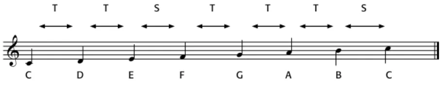
3.1 C major scale . . . 17 3.2 Harmonization of C major scale. Using only notes from the

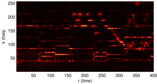
scale, we obtain a sequence of triads of different types. . . 18 3.3 Most used diatonic modes and their harmonization. . . 20 3.4 Steps of the Chromagram calculation . . . 23 3.5 Normalized spectrumA(r, k). r is the time index and k is the

frequency bin. In figure, for clarity, are showed only the first 256k of 4096. Only the first half (2048) of frequency bins are meaningful, as the transform of a real signal is symmetric. . . 24 3.6 Simple and complex pitch profiles matrices. k is the frequency

bin index andm is the pitch index. . . 25 3.7 Windows for bass and treble range chromagrams . . . 27 3.8 Treble and bass chromagrams . . . 27 3.9 State transition graph representation of hidden Markov

Mod-els. Nodes are states and allowed transitions are represented as arrows. . . 30 3.10 Hidden Markov Models are often represented by a sequence of

temporal slices to highlight howqt, the state variable at time

t, depends only on the previous one qt−1 and the observation

symbol at time t depends only on the current state qt. The

standard convention uses white nodes for hidden variables or states and shaded nodes for observed variables. Arrows be-tween nodes means dependence. . . 31 3.11 A directed acyclic graph . . . 32 3.12 Construction of a simple Dynamic Bayesian network, starting

from the prior slice and tiling the 2TBN over time. . . 34 XI

(16)

information is extracted by our beat tracker. Harmony-related information is extracted by our chord-recognition subsystem. These information are middle level features and are addressed to musically trained users. Harmony-related features are then extracted starting from key and chord information, and is ad-dressed to a generic user (no training needed). . . 36 4.2 Beat tracking system . . . 37 4.3 Signal s(n) and detection function η(m). The two functions

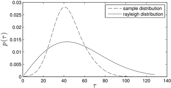
have different temporal resolutions but corresponding indices n and m are aligned in the figure for better understanding. . 39 4.4 Tempo estimation stage . . . 39 4.5 Comb filter matrixF . . . 41 4.6 Rayleigh distribution function with β = 43 compared to the

sample distribution of periods in our dataset . . . 41 4.7 Rhythmogram matrixyi(τ ). τ is the beat period expressed in

number of samples of the ODF. . . 42 4.8 Period transition distribution extracted from the dataset . . . 43 4.9 Rhythmogram. Chosen peaks and final path are showed

re-spectively as light and dark x.τ is the beat period expressed in number of samples of the ODF. . . 43 4.10 The performance of the beat tracking algorithm is influenced

byNpeaks . . . 44

4.11 Beat candidates cj are the highest peaks within each region,

marked with a cross. η(m) is the onset detection function and m is its time-intex . . . 45 4.12 Beat tracking stage . . . 45 4.13 Join and split rules applied to 6 path at the first 3 iterations . 47 4.14 Increasing the number of paths (Np = 2, 6, 10 in the figures)

influences the coverage of the space . . . 48 4.15 The performance of the beat tracking algorithm is influenced

byNp . . . 48

4.16 Precision and recall parameters plotted against the threshold tv 49

4.17 m is the sample index of tempo tracking songs and τ (m) is the estimated periodicity, expressed in number of ODF samples. At each iteration the algorithm smooths the tempo path in segments with least voted beats (most voted one are marked with an X). This way it can effectively correct the two tempo peaks, mistakenly detected by the earlier tempo tracking stage. 50

(17)

4.18 Performance of the algorithm slightly increase with the num-ber of iterations . . . 50 4.19 The spectral difference function for downbeat detection has

one value per beat. n is the audio sample index and m is the beat index. The two functions have different temporal resolutions but corresponding indicesn and m are aligned in the figure for better understanding. . . 51 4.20 The chroma variation function . . . 53 4.21 Performances of downbeat tracking stage are maximized for a

regularity parameter α = 0.5 . . . 54 4.22 Chord recognition scheme . . . 55 4.23 Beat-synchronized bass and treble chromagrams. . . 57 4.24 The two-slice temporal Bayes net of our chord tracking

sys-tem. Where shaded nodes are observed and white node are the hidden states nodes. L stands for beat label, and it rep-resents beat labels assigned during downbeat detection. K is the Key node, C the Chords node, B the bass note node, CB

is the Bass beat-synchronized Chromagram and S the chord salience node. . . 58 4.25 The pitch profile k∗(p) obtained from the dataset. . . 61 4.26 Norwegian Wood is a great example to show the power of

the Modal Envelope descriptor. Verses of the song are in Mixolydian mode and Choruses are in Dorian mode. The descriptor perfectly and precisely follows the shift in mood of the song. In this particular case it also achieve optimal structural segmentation . . . 63 4.27 Finer modal envelope feature obtained by a post-processing

of chords. The song is "Angel" by Robbie Williams. Spikes from major mode to mixolydian mode reveal where the com-poser made use of modal interchange. The longer zones are instead temporary modulations (key change) to the parallel mixolydian mode. . . 64 4.28 This function is a time window used to compute the

majMin-Feature. The rationale is simple: just listened events have a stronger influence than those happened before. . . 65 4.29 The figure shows an example of the majMinFeature on the

song "Hard Day’s Night" by The Beatles. The deepest valleys fall exactly at the choruses, where most minor chords are found. 66

(18)

The longest peaks represents parts of the song where chords changes are very frequent. . . 67 5.1 Continuously correct segments are showed as grey rectangles,

the longest is darker. CM Lt= 0.951 and CM Lc= 0.582 . . . 70

(19)

List of Tables

3.1 Pitch classes and their names. ] and [ symbols respectively rise and lower the pitch class by a semitone. . . 16 3.2 Pitches are related to their frequency using the standard

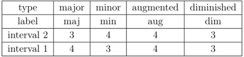
ref-erence frequencyA4 = 440Hz. . . 17 3.3 Sequence of tones and semitones in the major scale . . . 17 3.4 The four triad types. Intervals are specified in number of

semitones. . . 18 3.5 Relationships of major scale notes with the tonic . . . 18 3.6 Diatonic modes can be viewed as built sliding towards right a

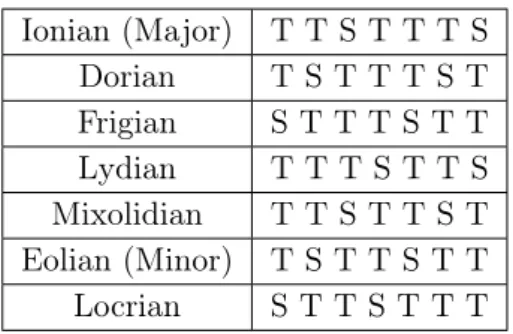
window over the major scale pattern. . . 19 3.7 Diatonic modes . . . 19 3.8 Examples of representative songs for the four main diatonic

modes . . . 19 3.9 Diatonic modes . . . 21 3.10 Diatonic modes . . . 21 4.1 Performances of sum of squared differences (SSD) and KL

Divergences (KLD) . . . 52 4.2 Signature distribution and transition probabilities . . . 53 4.3 Moods consistently associated with major and minor triads. . 64 5.1 Performances on the Beatles Dataset . . . 71 5.2 Performances on the Robbie Williams Dataset . . . 71 5.3 Performances of downbeat tracking on The Beatles Dataset . 72 5.4 Performances of downbeat tracking on the Robbie Williams

Dataset . . . 72 5.5 Performances on The Beatles dataset. krmRCO is computed

mapping key mode sequences of our system to only major and minor modes, as they only are present in the ground truth annotations . . . 73

(20)

fully evaluate only our system . . . 74 5.7 Results of theρ index shows that in 5 of the 6 cases, there is

a direct proportionality between our feature and the annota-tions. ME stands for Modal Envelope, Mm for MajMinRatio, HR for Harmonic Rhythm . . . 75 A.1 Album IDs . . . 88

(21)

(22)

(23)

Chapter 1

Introduction

The advent and the diffusion of the Internet and its increasing bandwidth availability, the growing density of newer storage systems, led to a new era for digital multimedia content availability and consumption. Music is rep-resentative of this revolution thanks to audio digital format such as mp3, aac, flac and new affordable music production tools. Online music stores as iTunes and Amazon, social platforms as last.fm and soundcloud are facing a crucial need to efficiently store and organize music content in huge databases. This involves the creation of meaningful descriptors to perform media search, classification and suggestion. This task has initially been accomplished by manually tagging songs with high-level symbolic descriptors (context-based approach). This approach is not suited for dealing with massive and ever increasing collections and, by definition, lacks of objectivity. The need of ob-jective and automated paradigms to extract information directly from music signals (content-based approach) contributed to the birth of a new research area, named Music Information Retrieval (MIR), a branch of Multimedia Information Retrieval. MIR is a broad field of research that takes advantage of signal processing techniques, machine learning, probabilistic modelling, musicological and psychoacoustic theories. The fundamental layer for MIR applications is the extraction of features able to describe several characteris-tics of musical content. These are generally categorized in three levels [15]. Low-level features (LLF) are directly extracted from the audio signal using signal processing techniques. Mid-Level features (MLF) make use of LLF and musicological knowledge to infer descriptors such as Melody, Harmony and Rhythm 1_{. High-level features have a higher degree of abstraction and}

are easily understandable by humans, like affective descriptors - emotional 1

These tasks and others are the object of Music Information Retrieval Evaluation eXchange (MIREX) annual evaluation campaign.

(24)

tags or continuous spaces as arousal, valence, dominance - and non-affective descriptors as genre, dynamicity, roughness, etc.

In this thesis we will focus on the Mid level. Particularly we will address the problem of automatic beat tracking and chord recognition. Further-more we propose three novel features computed from the extracted chord-progression by exploiting musicological background. We will then correlate these features to the emotion variation perceived in a song.

1.1 Beat Tracking and applications

Beat tracking is one of the most challenging task in the context of MIR field. Beat is a steady succession of pulses of that humans tend to follow when listening to a song.

Rhythm, as almost all aspects of music, is a hierarchical structure. It’s common to consider three metrical levels. Tatum is the lowest level of this hierarchy. The next level is the beat level or tactus, the period at which most humans would tap their foot or snap their fingers. The last and highest level is the measure level. Measure is a segment of time defined by a given number of beats. Downbeats are the first beats of each measure.

Extracting beat from audio is very useful for many applications. Beat information, for example, can be exploited in subsequent beat-synchronous analysis (sampling informations using the time-grid given by beats), in score alignment and chromagram synchronization for chord recognition, as we will see later on. Beat-synchronous processing can have applications in time-stretching. Professional DJ softwares make use of beats position and tempo information to help the user making rhythmically smooth cross-fades be-tween songs. In the music production field, music engineers can take great benefit from automatic slicing a track based on auto-detected beat instants, and then quantizing them to obtain a version with a steadier rhythm. A sequencer can vice versa adjust the tempo grid according to a track. Tempo, the period of the beats, can also be useful for automatic song library tagging. One of the id3 tags is in fact named beat per minute (bpm), and it indicates the average tempo of a song.

The downbeat extraction task has also many applications. Rhythmic pat-tern analysis can greatly benefit having a predefined grid over which to apply pattern recognition techniques. Downbeat positions can be also exploited as most likely temporal boundaries for structural audio segmentation.

Main techniques for beat-tracking work on an Onset Detection Function (ODF), extracted from the audio signal. This function is tailored as to highlight the transients and the start of new notes. Periodicities of this

(25)

1.2. Chord Recognition 5

function represent the tempo. The ODF is then scanned to find a regular pattern of peaks spaced by the tempo. The search of downbeat is carried out by finding regular patterns among the beats, with periodicities of three or four beats.

In this thesis we propose a new beat sequence technique based on a new multipath tracking algorithm based on dynamic programming, aware of tempo changes. This novel technique increases accuracy in beat track-ing by exploittrack-ing an iterative self evaluation. The same algorithm has been applied to downbeat detection with dynamic time signature tracking.

1.2 Chord Recognition

Automatic chord recognition task aims at generating chord transcriptions as similar as possible to those of highly trained musicians. Unlike beat-tracking, this isn’t an easy task for hobby musicians too. However, chords are important for modern pop music, given they provide alone enough infor-mation to allow musicians of any level to perform a recognizable version of a song. This is confirmed by a great demand for chord transcriptions on the Internet, where some web sites provide archives of home-made transcriptions submitted by users.

Aside from automatic transcription, the chord-recognition task encompass similarity-based applications like score synchronization and cover identifica-tion, and is used for genre classification as well. The harmony of a song is also connected to mood. Many psychoacoustic researches demonstrate how sensi-tive humans are with respect to harmonic structure. Chord progressions can influence mood in many ways, mainly by exploiting specific patterns linked to known emotional responses in the listeners. Sloboda [40] showed the bounds between harmonic patterns such as cycle of fifths, unprepared harmony or cadences, with responses as tears, shivers and racing heart. This is exactly what the composer does while writing a song, he searches the right balance to achieve a precise emotional meaning, often in tune with other layers as lyrics, arrangement or melody.

Harmony is not an exception in being a hierarchical structure, as rhythm is. Above the chords level is the key level. In tonal music, as is the vast majority of the music, one note, called tonic or key root, has greater im-portance than others. Other notes and chords have meaning in relation to the tonic, that is consequently said to provide a context. The relationships between notes and the key root, as we will see in chapter 3, form the key mode, one of the main aspects that induce mood in the listener.

(26)

addressed by creating probabilistic models or by filtering the chromagram in the time direction.

The goal of this thesis is to exploit diatonic modal harmony theory in order to improve chord transcription. We provide a novel parametric probabilistic modelling of chords and keys. Our model include all the four main key modes and not only the major and minor modes. Finally we exploit key mode and chord structure to extract harmony-related feature.

1.3 Thesis Outline

In chapter 2 we present some related works, representative of the state of the art in beat tracking and chord recognition techniques. Chapter 3 provides the theoretical background of algorithms and probabilistic models we use throughout our system. In chapter 4 attention is drawn to our system and we fully review each stage of beat and chord detection. Experimental results and comparison to existing systems is presented in chapter 5.

(27)

Chapter 2

State Of Art

In this chapter we will give an overview of the main existing approaches of beat tracking and chord recognition. The analysis will be subdivided in successive steps representing the common procedures in performing these tasks.

2.1 State Of Art in Beat Tracking

In this section we review the main existing approaches on the beat-tracking task. We split the analysis following the order of the building blocks of a standard beat-tracking system. Generally beat tracking task is divided in these successive steps:

• An Onset Detection Function (ODF) is generated from the input signal • Periodicities in the ODF are highlighted in the Rhythmogram

• Beat positions are detected starting from the ODF and the Rhythmo-gram

• Downbeats are found between beats 2.1.1 Onset detection function

Most of the beat tracking algorithms are based on a mono-dimensional fea-ture called Onset Detection Function (ODF) [4]. ODF quantifies the time-varying transientness of the signal where transients are defined as short in-tervals during which the signal evolves quickly in a relatively unpredictable way. More exaustive explanation of ODF will be given in Chapter 4.

Human ears cannot distinguish between two transients less than 10 ms apart, so that interval is used as the sampling period for ODFs. The process

(28)

of transforming the audio signal (44100 samples/s) to ODF (100 samples/s) is called reduction. Many approaches have been proposed for reduction. Some make use of temporal features as envelope [38] or energy. Others take into account the spectral structure, exploiting weighted frequency magnitude. In[28], for example, a linear weightingWk=|k| is applied to emphasize high

frequencies. Different strategies have advantages with different types of mu-sical signals. We choose the spectral difference detection function proposed by [2] as the state of art for pop songs.

2.1.2 Tempo estimation

Periodicities in the ODF represent beat period or tempo of the song and are searched using methods as auto-correlation, comb-filter resonator or short-time Fourier Transform (STFT). A spectrogram-like representation of such periodicities is called Rhythmogram (Fig. 4.7). This task, concerning the beat rate instead of beat positions, takes the name of tempo estimation. In [12] was proposed a very effective way to find periodicities using a shift-invariant comb filter-bank. Tempo generally varies along the piece of music. The analysis is, therefore, applied at windowed frames of 512 ODF samples, with 75% overlap. One of the main problem, at this level is the trade off between responsiveness and continuity. In [12] this problem was assessed using a two state model, in which the "General State" takes care of respon-siveness and the other, called "Context-Dependent State", try to maintain continuity.

2.1.3 Beat detection

The beat detection phase addresses the problem of finding the positions of beat events in the ODF. A simple peak picking algorithm would not be sufficient as there are many energy peaks that are not directly related to beats. Human perception as a matter of fact tends to smooth out inter-beat-intervals to achieve a steady tempo. This can be modelled, as proposed in [13], by an objective function that combines both goals: correspondence to ODF and interval regularity. Inter-beat-interval is the tempo, so it is derived from an earlier tempo detection stage. An effective search of an optimal beat sequence_{ti} can be done in a simple neat way by assuming tempo as given

and using a dynamic programming algorithm technique [1].

Irregularities in the detected tempo path are one of the main sources of error. We propose a novel beat-tracking technique that track simultaneously more likely beat sequences. In doing so it manages to identify and correct

(29)

2.2. State Of Art in Chord Recognition 9

some of the errors carried on from earlier stages, mainly the tempo estimation stage.

2.1.4 Time signature and downbeat detection

Downbeat detection stage focuses on the highest level of rhythmic hierarchy. Outputs of this stage are the set of the first beats of each measure. As inter-beat-intervals sequence constitute the tempo, inter-downbeat-intervals, expressed in beats per measure, represents the time signature. Common time signatures are 4/4 and 3/4 meaning respectively four beats per measure and three beats per measure. In [17] a chord-change probability function is exploited in making decisions on higher level beat structure. In [16], bass drum and snare drum onsets are detected by a frequency analysis stage. Patterns formed by these onsets and their repetitions are used as cues for detecting downbeats. The algorithm used as the state of art is described in [11]. The input audio is down-sampled and a spectrum is calculated for every beat interval. A spectral difference function D is then obtained by Kullback-Leibler divergence between successive spectra. This function gives the probability that a beat is also a downbeat. Downbeat phase is then found by maximizing the correlation ofD with a shifting train of impulses.

Our model exploits the same multipath algorithm to track the sequence of downbeats among beats. It exploits, as the downbeat’s ODF, a combination of an energy based feature and a chroma variation function.

2.2 State Of Art in Chord Recognition

In this section we review the existing approaches in Chords and Keys ex-traction. Again, we split the analysis following the major steps undertaken by a standard algorithm starting from the audio signal.

2.2.1 Chromagram extraction from audio domain

Most of the chord-recognition algorithms are based on a vectorial feature called Chromagram, which will be described in detail in chapter 3. Chroma-gram is a pitch class versus time representation of the audio signal [43]. It is computed starting from Spectrogram by applying a mapping from linear to log-frequency. This procedure is most often accomplished by the constant-Q transform [5].

For the task of chord-recognition, Chromagram is needed to show the relative importance of pitch classes of notes played by instruments. The

(30)

Spectrogram, however, contains noise coming from percussive transients and contains harmonics (tones at integer multiples of the fundamental frequency of a note). Furthermore the overall tuning reference frequency may not be the same for all songs. It’s therefore necessary to develop strategies and work-arounds to cope with these problems.

2.2.2 Chromagram enhancement

The basic approach in reducing percussive and transient noise is to apply a FIR low pass or a median filter to the Chromagram in the time axis. The same result is achieved as a side-effect of beat-synchronization, that consists in averaging Chroma vectors inside every beat interval. Beat-synchronization is usually performed in chord-recognition as proposed in [3]. Other methods include spectral peak picking ([18]) and time-frequency reassignment ([24]). The Harmonics contribute to characterize the timbre of instruments but are not perceived as notes and have no role in chord perception. For the chord-recognition task therefore, their contribute is undesirable. To address this issue, in [18], spectral peaks found in the spectrogram contribute also to sub-harmonic frequencies, with exponentially decreasing weight. In [29] each spectrogram frame is compared to a collection of tone profiles containing harmonics.

For historical reasons the frequencies of the notes in our tuning system, the twelve-tone equal temperament, are tuned starting from the standard reference frequency of a specific note: A4 = 440Hz. This frequency in some songs vary in the interval between 415 Hz and 445 Hz, then it is necessary to determine it to obtain a reliable chromagram. The approach generally used is to generate a log-frequency representation of the Spectrogram with frequency resolution higher than the pitch resolution. In [21] 36 bins per octave are extracted. The same resolution is achieved with pitch-profiles collection matrices in [30]. Since our temperament has 12 pitch classes per octave, we obtain 3 bins per pitch. Circular statistics or parabolic interpo-lation allow us to find the shift of the peak from the centre bin, hence the shift of the reference frequency.

2.2.3 Chord Profiles

Chord recognition is achieved by minimizing a distance or maximizing a similarity measure between the time slices of the Chromagram and a set of 12-dimensional pitch class templates of chords. Chord theory and derivation of pitch class templates is treated in full detail in the next chapter. Inner

(31)

2.2. State Of Art in Chord Recognition 11

product is used as a similarity measure in [21]. In [34] the use of Kullback-Leibler divergence as a distance measure is proposed. In [3], chords template vectors are centre-points of 12-dimensional Gaussian distribution with hand tuned covariance matrices.

2.2.4 Chord sequences

Finding a chord for each slice of the Chromagram would result in a messy and chaotic transcription, useless from any musical point of view. This is caused by 2 main factors: the percussive transients that results in a wide non-harmonic spectrum, and the melody notes and other non-chord passing notes that can make the automatic choice of the right chord an hard task. To obtain a reliable and musically meaningful chord transcription we must account for the connections and hierarchies of different musical aspects.

Chords are stable in a time-interval of several seconds. It is then necessary to find a strategy to exploit this evidence and find smooth chords progres-sions over time. A segmentation algorithm proposed in [14] uses a "chord change sensing" procedure that computes chord changes instants by apply-ing a distance measure between successive chroma vectors. In [21] a low pass filtering of chroma frames and then a median filtering of frame-wise chord labels is performed. In [34] the smoothing is applied not to the labels but on the frame-wise score of each chord. The majority of chord transcription algorithm use probabilistic models as Hidden Markov Models (HMMs), ex-plained in chapter 3, which are particularly suited for this task as they model sequences of events in a discrete temporal grid. In HMMs for chord recog-nition task, chords are the states and chroma vectors are the observations. The model parameters as the chord transitions and the chroma distribution for each chord express musically relevant patterns.

Chroma distributions are mainly based on chord profiles. One of the most important parameters is the self-transition, which models the probability that a chord remains stable. Between approaches exploiting HMMs, [3] is notable as the chord transition matrix is updated for each song, starting from a common base, that model the a-priori common intuition of a human listener. Another probabilistic model recently used [27] in the MIR field is the Dynamic Bayesian Network (DBN) [32], reviewed in chapter 3. DBN can be seen as a generalization of HMM that allows to model, besides chord transition patterns, any other type of musical context in a network of hidden and observed variables.

(32)

2.2.5 Musical contexts

Other musical context used along with chord transition patterns are Key, Metric position, and Bass note contexts.

The fundamental importance of Key in human perception of harmonic relationships is highlighted in chapter 3. This has been exploited success-fully in many chord recognition systems. Some of them [39] use the Key information to correct the extracted chord sequence, others [6] try to extract the Key simultaneously to the chord sequence. The Key changes, or mod-ulations, in a song are addressed only by some of the existing approaches, while the majority of them assumes the Key to remain constant throughout the song. The key modes addressed by these systems are major and minor modes.

Bass note (the lowest note of a chord) can be estimated by creating a sep-arated Bass-range Chromagram that include only the low frequency pitches. The pitch class of the Bass note is likely to be a note of the chord. This as-sumption is exploited in [31] by creating a CPD of chords given a bass-range chroma vector.

Metric position can also be used as a context, exploiting the fact that chord changes are likely to be found at downbeat positions, as done in [35]. We propose a novel probabilistic model of keys that include, besides major and minor modes, the Mixolydian and the Dorian mode. The parameters of this model express meaningful events as different types of modulations. Furthermore, we propose a new conditional probability model of chords, given the key context. This model assigns three different parameters to different group of chords, based on the key mode and the relationship with the tonic.

2.2.6 Key Extraction

Key extraction is usually done by comparing Chroma vectors with a set of key templates. Correlation is used as similarity measure as in [18]. HMMs are used to track the evolution of key in a song. The best known key tem-plates (the concept of key and tonality is reviewed in the chapter 3) are the Krumhansl’s key profiles ([26]). They contains 12 values that show how pitch classes fit a particular key. This profiles were obtained by musicological tests and, as expected, agree with music theory. Krumhansl’s key profiles are available for major and minor keys. Other key profiles are automatically extracted in [7] from a manually annotated dataset of folk songs.

To compute the keys we propose a hybrid system. It first weights our a-priori probability model by a vector of key root saliences, obtained by

(33)

correlating the chromagram with a set of key root profiles. Then the keys sequence is extracted together with chord sequence by viterbi inference for the Dynamic Bayesian Network.

(34)

(35)

Chapter 3

Theoretical Background

In this chapter we will review the theoretical background and tools used in our technique. We will begin with the basic musical background needed to understand chords, keys and key modes. Then, we will introduce two low level signal processing tools, the Short Time Fourier Transform (STFT) and the Chromagram. Successively, we will explain the main concepts of the probabilistic models we used in the beat tracking system: the Hidden Markov Models (HMM). Finally we will review a generalization of HMM, the Dynamic Bayesian Network (DBN): the probabilistic model that will be used in the chord recognition system to model a number of hidden state variables and their dependencies.

3.1 Musical background

In this section we review some basic concepts of music theory. In particular we cover what is pitch and pitch classes, how chords are formed and their relation to key and modes. For a comprehensive reference we remind the reader to [44].

3.1.1 Pitch and pitch classes

Pitch is a perceptual attribute which allows the ordering of sounds on a frequency-related scale extending from low to high ([25]). Pitch is propor-tional to log-frequency. In the Equal temperament it divides each octave (a doubling of frequency) in 12 parts:

fp = 2

1

12f_p−1. (3.1)

wherefp is the frequency of a note . In this study pitch and note terms are

used as synonyms from now on. The distance between two notes is called 15

(36)

interval, and is defined by a frequency ratio. The smallest interval, called semitone, is defined by the ratio

fp

fp−1

= 2121 . (3.2)

An interval of n semitones is therefore defined by 212n. The interval of 2 semitones is called tone.

Human are able to perceive as equivalent pitches that are in octave re-lation. This phenomenon is called octave equivalence. Pitch classes are equivalence classes that include all the notes in octave relation. Note names indicates, in fact, pitch classes (Table 3.1).

note name pitch class #

C 1 C]/D[ 2 D 3 D]/E[ 4 E 5 F 6 F]/G[ 7 G 8 G]/A[ 9 A 10 A]/B[ 11 B 12

Table 3.1: Pitch classes and their names. ] and [ symbols respectively rise and lower the pitch class by a semitone.

Octave is indicated by a number after the pitch class. In Table 3.2 pitches are related to their frequency in the the Equal temperament, tuned relative to the standard reference: A4 = 440Hz.

(37)

3.1. Musical background 17 Octave Note 2 3 4 5 6 C 66 Hz 131 Hz 262 Hz 523 Hz 1046 Hz C]/D[ 70 Hz 139 Hz 277 Hz 554 Hz 1109 Hz D 74 Hz 147 Hz 294 Hz 587 Hz 1175 Hz D]/E[ 78 Hz 156 Hz 311 Hz 622 Hz 1245 Hz E 83 Hz 165 Hz 330 Hz 659 Hz 1319 Hz F 88 Hz 175 Hz 349 Hz 698 Hz 1397 Hz F]/G[ 93 Hz 185 Hz 370 Hz 740 Hz 1480 Hz G 98 Hz 196 Hz 392 Hz 784 Hz 1568 Hz G]/A[ 104 Hz 208 Hz 415 Hz 831 Hz 1661 Hz A 110 Hz 220 Hz 440 Hz 880 Hz 1760 Hz A]/B[ 117 Hz 233 Hz 466 Hz 932 Hz 1865 Hz B 124 Hz 247 Hz 494 Hz 988 Hz 1976 Hz

Table 3.2: Pitches are related to their frequency using the standard reference frequency A4 = 440Hz.

Scales are sequences of notes that cover the range of an octave. Scales are classified based on the intervals between successive notes. The particular sequence of semitone and tone intervals depicted in the Table 3.3 compose the major scale (Fig. 3.1).

T T S T T T S

Table 3.3: Sequence of tones and semitones in the major scale

& œ œ œ œ œ œ œ œ

T T S T T T S

C D E F G A B C

Figure 3.1: C major scale

3.1.2 Chords

Chords are the combination of two or more intervals of simultaneous sound-ing notes. Chords are classified by their number of notes and the intervals between them.

(38)

The most used chord type in western pop music is the triad. Triads are three note chords, and divide in 4 types depending on the intervals between their notes (Table 3.4).

type major minor augmented diminished

label maj min aug dim

interval 2 3 4 4 3

interval 1 4 3 4 3

Table 3.4: The four triad types. Intervals are specified in number of semitones.

We can build a triad on each note of the major scale, using only scale notes. This process is called harmonization of the major scale. We obtain the series of triads showed in Fig. 3.2.

& œœœ œœœ œœœ œœœ œœœ œœœ œœœ œœœ

C:maj D:min E:maj F:maj G:maj A:min B:dim C:maj

Figure 3.2: Harmonization of C major scale. Using only notes from the scale, we obtain a sequence of triads of different types.

3.1.3 Tonal music and keys

Music is tonal when a pitch class more important than others can be outlined. This pitch acts as centre of gravity and is called tonic or key root. The tonic is the most stable pitch class where to end a melody, to obtain a final resolution (think of any western national anthem). The triad built on the tonic is the most likely chord where to end a song. Most of the western music is tonal.

The concept of key mode relates to the particular choice of other notes in relation with the key root. A mode correspond to a scale in the sense that notes are taken from a particular scale of the key root. For example, given the intervals pattern of the major scale (Table 3.3), the pattern of intervals of scale notes with the key root is

T T S T T T S

2 4 5 7 9 11 12

(39)

3.1. Musical background 19

Most used modes are taken from a set of scales called the diatonic scales that include the circular shifts of the major scale. They are therefore called diatonic modes.

... T T S T T T S T T S T T T S T T S T T T S ...

Table 3.6: Diatonic modes can be viewed as built sliding towards right a window over the major scale pattern.

Ionian (Major) T T S T T T S Dorian T S T T T S T Frigian S T T T S T T Lydian T T T S T T S Mixolidian T T S T T S T Eolian (Minor) T S T T S T T Locrian S T T S T T T

Table 3.7: Diatonic modes

Most used modes in western music (Table 3.8) are Major, Mixolydian, Dorian and Minor. Their scale and set of triads, in the key root of C, are showed in Fig. 3.3.

Major Mixolydian

Imagine (John Lennon) Sweet Child Of Mine (Guns ’n’ Roses) Blue Moon (Rodgers, Hart) Don’t Tell Me (Madonna)

We are golden (Mika) Teardrop (Massive Attack)

Something Stupid (Robbie Williams) Millennium (Robbie Williams)

Dorian Minor

I Wish (Steve Wonder) Losing My Religion (REM)

Oye Como Va (Santana) Rolling In The Deep (Adele) Great Gig In The Sky (Pink Floyd) Have a Nice Day (Bon Jovi)

Mad World (Gary Jules) I Belong To You (Lenny Kravitz)

Table 3.8: Examples of representative songs for the four main diatonic modes

In western music, modes have been shown to be linked with emotions, as for instance minor modes are related to sadness and major to happiness ([22]). If we evidence the intervals with key root for each diatonic mode, we can order them by the number of risen and lowered notes (Table 3.9).

(40)

& œ œ œ œ œ œ œ œ

T T S T T T S

C D E F G A B C

& œœœ œœœ œœœ œœœ œœœ œœœ œœœ œœœ

C:maj D:min E:maj F:maj G:maj A:min B:dim C:maj

(a) C Major scale and its harmonization

& œ œ œ œ œ œ œb œ

T T S T T S T

C D E F G A Bb C

& œœœ œœœ œœœb œœœ œœœb œœœ œœœb œœœ

C:maj D:min Eb:dim F:maj G:min Ab:min Bb:maj C:maj

(b) C Mixolydian scale and its harmonization

& œ œ œb œ œ œ œb œ

T S T T T S T

C D Eb F G A Bb C

& œœœb œœœ œœœbb œœœ œœœb œœœb œœœb œœœb

C:min D:min Eb:maj F:maj G:min A:dim Bb:maj C:min

(c) C Dorian scale and its harmonization

& œ œ œb œ œ œb œb œ

T S T T S T T

C D Eb F G Ab Bb C

& œœœb œœœb œœœbb œœœb œœœb œœœbb œœœb œœœb

C:min D:dim Eb:maj F:min G:min Ab:maj Bb:maj C:min

(d) C Minor scale and its harmonization

(41)

3.2. Audio features analysis 21

Lydian 2 4 6 7 9 11 12 1 risen note brightest Ionian (major) 2 4 5 7 9 11 12

-Mixolidian 2 4 5 7 9 10 12 1 lowered note Dorian 2 3 5 7 9 10 12 2 lowered notes Eolian (minor) 2 3 5 7 8 10 12 3 lowered notes Frigian 1 3 5 7 8 10 12 4 lowered notes

Locrian 1 3 5 6 8 10 12 5 lowered notes darkest

This ordering, not the circular shift one, is relevant from an emotional point of view. We believe it is consistent with a direction in the emotional meaning of the modes. We can notice how the four most used modes are in central positions. A collection of keywords used to describe emotions in these four modes is provided in Table 3.10 [23].

Major Mixolydian Dorian Minor

happiness bluesy soulful sadness brightness smooth hopeful darkness

confidence funky holy defeat

victory folky moon tragedy

3.2 Audio features analysis

In this section we will give a review of basic signal processing tools we will need in the next chapter. These tools are needed to extract low level fea-tures directly from the audio samples domain. Short-Time Fourier Trans-form (STFT) is a Fourier-related transTrans-form that computes a frequency-time representation of the signal, needed to calculate the Onset Detection Func-tion in the beat-tracking system. Chromagram is a pitch-class versus time representation of the signal. It is a prerequisite for chord recognition and is obtained from the STFT.

3.2.1 Short-Time Fourier Transform

Short-Time Fourier Transform (STFT) is a Fourier-related transform used to determine the sinusoidal frequency and phase content of local sections of a signals(n) as it changes over time (n is the sample index). It is computed by dividing the signal into frames by multiplication by a sliding window w(n)

(42)

(w(n)6= 0 for 0 ≤ n ≤ Lw− 1) and Fourier-transforming each frame. Three

parameters are specified: transform-size NF T, window length Lw < NF T

and hop-sizeH. The equation is

Sr(ωk) = NF T−1 X n=0 (s(n− rH)w(n))e−jωkn _{k = 0, ..., N} F T, (3.3)

whereωk = 2πk/NF T is the frequency specified in [rad/s],r is frame index,

k is the frequency bin. Usually Lw = NF T = 2η, because the Fourier

trans-form is computed by the fast implementation called Fast Fourier Transtrans-form (FFT), that has maximized performances for power of 2 transform sizes. For real valued signals the Fourier transform is symmetric, then we consider only the first half of the spectrum (k = 0, ..., NF T/2− 1). Sampling in the time

axis is controlled by the hop-size parameterH. The parameter NF T is linked

to frequency resolution∆f = fs/NF T wherefsis the sampling frequency of

the s(n). Frequency resolution however must account also for the effect of convolution with the Transform of the window functionW (ωk) due to

mul-tiplication in the time-domain. We will need to account this concept when choosing NF T large enough to obtain the resolution needed to distinguish

two tones at certain frequency. Sometimes only the magnitude information is needed so a matrix representation called Spectrogram,P (r, k) =_|Sr(ωk)|2,

is used instead.

3.2.2 Chromagram

Chromagram describes how much the pitch-classes are present in a frame of the audio, then is a pitch-class versus time representation. In our chord-tracking system it will be compared with chord templates to find which chord is playing at a given time.

To compute the Chromagram we follow a series of steps (Fig. 3.4). First we extract the STFT from audio, then we compare the magnitude spectrum with a series of pitch profiles. We obtain the pitch salience representation that indicates how much the pitches are present in the audio frame. We then perform noise reduction to retain only significant peaks and discard the noise due, for example, to percussive transients. Successively we perform tuning to compensate the potential offset from the standard A4 = 440Hz reference. Finally bass and treble Chromagram are separated to later exploit the importance of the bass note in the chord-recognition system.

(43)

3.2. Audio features analysis 23

STFT Pitch

saliences

Noise

reduction Tuning

Bass & Treble Mappings

Figure 3.4: Steps of the Chromagram calculation

Frequency-Domain Transform

First of all we must compute the STFT of the signal. Fundamentals of notes from C0 to C7 lie in the range of _{∼ [30, 2000]Hz then we can down-sample} the audio signal tofs= 11025 Hz without loss of information. Furthermore

we must ensure that we achieve the desired frequency resolution. The lower limit ofNF T is given by

NF T > K

fs

|f2− f1|

, (3.4)

where K is a parameter that depends on the window function used, for Hamming window K = 4. We want the frequencies of A3 and G]3 to be discernible, soNF T has to satisfy

NF T > 4

11025

|220 − 208| = 3675. (3.5)

The minimum (to save computation time) power of 2 that satisfy this require-ment is212_{= 4096. So we compute the STFT of the signal with N}

F T = 4096

and normalize each time slice with respect toL2 norm (Fig.):

A(r, k) = |Sr(ωk)| (P

q|Sr(ωq)|2)1/2

(3.6)

Pitch salience

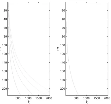
To construct the time-pitch representation and simultaneously account for harmonics in timbre of instruments we adopt the approach proposed in [18] and modified in [29]. We construct a pitch profile matrixMc_{(Fig. 3.6),}

simi-lar to a constant-Q transform kernel, where each row is the Fourier transform of a Hamming windowed [41] complex tone, containing four harmonics in ge-ometric amplitude sequence.

Mc(m, k) = F F TNF T(w(n)

4

X

h=1

(44)

k (freq) r (time) 50 100 150 200 250 300 350 400 50 100 150 200 250

Figure 3.5: Normalized spectrumA(r, k). r is the time index and k is the frequency bin. In figure, for clarity, are showed only the first 256 k of 4096. Only the first half (2048) of frequency bins are meaningful, as the transform of a real signal is symmetric.

where α = 0.9, w(n) is the Hamming window and the fundamentals starts from the fundamental frequency of A0 (27.5 Hz) and are

f0(m) = 27.5× 2

m−2

36 m = 1, ..., 6× 36, (3.8)

where m is the pitch index. This means that our pitches span 6 octaves, from A0 to G]6, with the resolution of 1/3 semitone. This fine resolution will allow us to perform tuning at a later stage.

We obtain a pitch salience matrix Sc _{by multiplying} _{A by M}c_. _This

however leads to a problem because also sub-harmonics (pitches at f = f0/n) have high values. This is addressed by constructing another pitch

profile matrixMs _{similar to}_Mc _{but considering only a simple tone with no}

harmonics. Pitch salience matrices are obtained by

Sc(m, r) = Mc(m, k)A(k, r) Ss(m, r) = Ms(m, k)A(k, r), (3.9)

and passed to the next stage where they will be filtered and combined. Broadband noise reduction

To lower broadband noise we have to retain only peaks in both salience matrices. We threshold each time-slice and retain only values higher than the local mean plus the local standard deviation. This two statistics are computed considering an interval of half an octave. ThresholdedSc _and _Sc

(45)

3.2. Audio features analysis 25 k m 500 1000 1500 2000 20 40 60 80 100 120 140 160 180 200 k m 500 1000 1500 2000 20 40 60 80 100 120 140 160 180 200

Figure 3.6: Simple and complex pitch profiles matrices. k is the frequency bin index andm is the pitch index.

S_m,tpre=      Ss m,tSm,tc ifSm,ts > µsm,t+ σm,ts andSc m,t> µcm,t+ σm,tc 0 0 (3.10) Tuning

Having recovered the pitch salience matrix with three times the resolution needed, we can compensate for tuning shifts from the standard reference of 440 Hz, by performing circular statistics. To achieve a more robust tuning we exploit the fact that the tuning do not change within a song, so we can average all the temporal slices

¯ S = 1

T X

tS_m,tpre. (3.11)

To find the tuning offset find the phase of the complex number obtained by

c =X

m

¯

S(m)ej2π3 (m−1), (3.12)

and divide it by 2π to obtain the tuning shift in semitones: t = phase(c)

(46)

With this information we can interpolateSpre _{so that the middle bin of each}

semitone corresponds to the pitch estimated. Now the extra resolution of 1/36 semitone is not needed any more, so we sum the three bins for each semitone: Sn,t = 3n X m=3n−2 S_m,tpre. (3.14)

Bass and treble Chroma

As said, we need two chromagram representation for the different ranges. Given the importance of the bass note in the harmony, we will exploit the bass chromagram to increase the accuracy of chord detection.

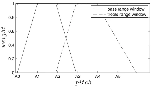
The bass and treble chromagrams (Fig. 3.8) are obtained by multiplying Sn,t by two windows functions wt(n) and wb(n) (Fig. 3.7), that satisfy 2

constraints:

• they sum to 1 in the interval from A1 to G]3

wt(n) + wb(n) = 1 13 < n < 48. (3.15)

• they give the a constant total weight to all the pitch classes P5

k=0(wt(12k + pc)) = ρt

P5

k=0(wb(12k + pc)) = ρb,

(3.16)

The two chromagrams are obtained by: CT p,t= P5 k=0wt(12k + p)S12k+p,t CB p,t= P5 k=0wb(12k + p)S12k+p,t (3.17)

A third version of the chromagram that we will use for creating the chord salience matrix, called wide chromagram CW_{, is obtained by summing the}

two.

C_p,tW = C_p,tT + C_p,tB. (3.18)

3.3 Dynamic programming

Dynamic programming (DP) is a technique for the design of efficient al-gorithms. It can be applied to optimization problems that generate sub-problems of the same form. DP solves sub-problems by combining the solutions

(47)

3.3. Dynamic programming 27 A0 A1 A2 A3 A4 A5 0 0.2 0.4 0.6 0.8 1

pitch

w

e

ig

h

t

bass range window treble range window

Figure 3.7: Windows for bass and treble range chromagrams

treble chromagram pitch classes time 500 550 600 650 700 750 C D E F G A B bass chromagram pitch classes time 500 550 600 650 700 750 C D E F G A B

(48)

to sub-problems. It can be applied when the sub-problems are not indepen-dent, i.e. when sub-problems share sub-sub-problems. The key technique is to store the solution to each sub-problem in a table in case it should reap-pear. The development of a dynamic-programming algorithm can be splitted into a sequence of four steps.

1. Characterize the structure of an optimal solution. 2. Recursively define the value of an optimal solution.

3. Compute the value of an optimal solution in a bottom-up fashion. 4. Construct an optimal solution from computed information.

A simple example is the assembly-line scheduling problem proposed in [8], which shares many similarities with beat-tracking algorithm in [13]. Let’s focus on beat tracking and see how DP can be applied to our problem.

Given a sequence of candidate beat instants t(i) with i = 1, ..., N , two specific functions can be formulated: O(i) and T (i). O(i) is an onset detec-tion funcdetec-tion and says how much a beat candidate is a good choice based on local acoustic properties. T (i) is the tempo estimation that describe the ideal time interval between successive beat instants. We search a optimal beat sequence t(p(m)) with m = 1, ..., M , such that onset strengths and correspondence to the tempo estimation is maximized.

As the first step let’s characterize the structure of the optimal beat se-quence that ends with the beat candidatet(iend). To obtain it, we must

eval-uate all the J sequences that end with tiend, that we represent ast(pj(m)) with pj(M ) = iend, and choose the best one t(pbest(m)). t(pbest(m)) will

surely contain the best sequence up to t(pj(M − 1)). The key is to realize

that the optimal solution to a problem contains optimal solutions to sub-problems of the same kind.

In the second step we have to recursively define the value of an optimal solution. The optimal beat sequence solution t(pbest(m)) will have to both

maximize P O(pbest(m)) and the probabilities of all the transitions. Let’s

define a single objective function C that combines both of these goals. C evaluates a sequencep(m) and returns a score:

C(p) = M X m=1 O(p(m)) + M X m=2 F (t(p(m))− t(p(m − 1)), T (p(m))) (3.19) where F is a score function that assign a score to the time interval ∆t between two beats, given an estimationT of the beat period. F is given by

(49)

3.4. Hidden Markov Models 29

this equation:

F (∆t, T ) =−(log∆t T )

2_. _(3.20)

The key property of this objective function is that the score of the best beat sequence up to the beati can be assembled recursively. This recursive formulation C∗ is given by:

C∗(i) = O(i) + max

prev=1,...,i−1(F (t(i)− t(prev), T (i)) + C

∗_(prev)) _(3.21)

The third step is another key point in dynamic algorithms. If we base a recursive algorithm on equation 3.21 its running time will be exponential in N , the number of beats in the sequence. By computing and storing C∗(p(m)) in order of increasing beat times, we’re able to compute the value of the optimal solution in Ω(N ) time.

Fourth and last step regards the actual solution. For this purpose, while calculatingC∗, we also record the ideal preceding beatP∗(i):

P∗(i) = arg max

prev=1,...,i−1(F (t(i)− t(prev), T (i)) + C ∗

(prev)) (3.22) Once the procedure is complete,P∗ allows us to retrieve the ideal preceding beat P∗(i) for each beat i. We can now backtrace from the final beat time to the beginning of the signal to find the optimal beat sequence.

3.4 Hidden Markov Models

In the MIR field is typical to characterize signals as statistical models. They are particularly useful for the recognition of sequence of patterns. One ex-ample are the hidden Markov Models(HMMs) [37]. Within beat tracking task, HMM can be used, for example, to find the tempo-path, given the Rhythmogram.

Markov models describe a system that may be in one ofN distinct states, S1, S2, ..., SN. After a regular specific quantum of time it changes the state,

according to a set of probabilities associated with the current state. Let’s denote the actual state at timet as qt. The probability of being in the state

qt= Sj given the previous stateqt−1= Si is given by

p(qt= Sj|qt−1= Si). (3.23)

In eq. 3.23, p is independent by the time, then we can gather those proba-bilities in a state-transition matrix with elements:

(50)

where aij ≥ 0, N X j=0 aij = 1,∀i. (3.25)

Markov models where each stateSj corresponds to an observable eventvjare

called observable Markov models or simply Markov Models. The three states model of the weather proposed in [37] is an example. The only parameters required to specify the model are the state-transition matrixA ={aij} and

the initial state probabilitiesπi = p(q1 = Si).

In contrast to Markov models, in hidden Markov Models, observations symbolsvk do not correspond to a state, but depend to the state, following

a series of conditional probability distributions CPDs bkj:

bkj = p(Ot= vk|qt= Sj), 1≤ j ≤ N, 1 ≤ k ≤ M, (3.26)

whereOt is the symbol observed at time t. An easy example is the tossing

ofN coins, differently biased, where each coin is a state Sj withj = 1, ..., N

and outcomes are the observationsvkwithk = 0, 1. HMM are fully specified

by the state-transition matrix A, the initial state probabilities π and the observation symbol CPDs B = _{bij}. The complete parameter set is then

indicated byλ = (A, B, π).

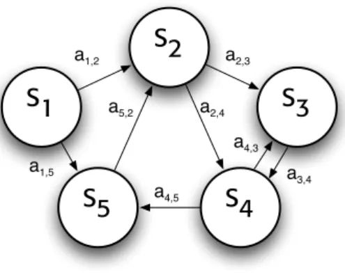
There are two main graphic representations of HMM. The first, called state-transition diagram, is a graph where node represent states and arrows are allowable transitions between them (Fig. 3.9). The second is a directed graphical model that shows variables in a sequence of temporal slices, high-lighting time dependencies (Fig. 3.10).

S5

S4

S1

S2

S3

a1,2 a2,3 a3,4 a4,5 a1,5 a5,2 a2,4 a4,3

Figure 3.9: State transition graph representation of hidden Markov Models. Nodes are states and allowed transitions are represented as arrows.

(51)

3.5. Viterbi decoding algorithm 31

q1

q2

q3

O1

O2

O3

π

A

B

t

Figure 3.10: Hidden Markov Models are often represented by a sequence of temporal slices to highlight howqt, the state variable at timet, depends only on the previous one

qt−1 and the observation symbol at timet depends only on the current state qt. The

standard convention uses white nodes for hidden variables or states and shaded nodes for observed variables. Arrows between nodes means dependence.

3.5 Viterbi decoding algorithm

The Viterbi algorithm is a formal technique, based on the dynamic program-ming method that finds the single best state sequence Q = _{q1, q2, ..., qT}

that maximize p(Q|O, λ), where O is the sequence of observations O = {O1, O2, ..., OT}. First we define in a recursive fashion the value or score

of a solution: we define the best score that ends to the state Si at timet as

δt(i) = max q1,q2,...,qt−1

p(q1, q2, ..., qt= Si|O1, O2, ..., Ot, λ) (3.27)

And find the recursive relationship δt+1(j) = max

i [δt(i)aij]bj(Ot+1) (3.28)

Then we compute this value from the start of the sequence, keeping track along the way of both sub-solution score δt(i) and best previous state ψt(i)

(needed for backtracking). These are computed for every time slice and for every state. The full procedure follows these four steps. Initialization

δ1(i) = πibi(O1) 1≤ i ≤ N (3.29)

ψ1(i) = 0 (3.30)

Recursion

δt(j) = max

(52)

ψt(j) = arg max i [δt−1(i)aij] 1≤ j ≤ N, 2 ≤ t ≤ T (3.32) Termination score = max i [δT(i)] (3.33) q_T∗ = arg max i [δT(i)] (3.34) Backtracking q_t∗= ψt+1(qt+1) t = T − 1, T − 2, ..., 1 (3.35)

3.6 Dynamic Bayesian networks

Dynamic Bayesian Networks (DBN) are a generalization of HMMs that al-lows the state space to be represented in factored form, instead of a single discrete random variable.

A Directed Acyclic Graph (DAG Fig. 3.11) is a set of nodes and edges G = (N odes, Edges), where Nodes are vertices and Edges are connections between them. Edges are directed if they imply a non-symmetric relation-ship, in this case the parent_{→son relationship. A graph is directed if all its} edges are directed. Acyclic means that it is impossible to follow a path from N odei that arrives back at N odei, as to say that N odei is an ancestor of

itself. Node 2 Node 1 Node 4 Node 5 Node 3

Figure 3.11: A directed acyclic graph

A Bayesian network (BN) is a directed acyclic graph whose nodes represent a set of random variables_{X1:N}, where N is the number of nodes, and whose

edge structure encodes a set of conditional independence assumptions about the distribution P (X1:N):

(53)

Under these assumptions, and if the set _{X1:N} is topologically ordered

with parents preceding their children,P (X1:N) can be factored as the

prod-uct of local probabilistic modelsP (Xi|P arents(Xi)):

P (X1, ..., XN) = N

Y

i=1

P (Xi|P arents(Xi)). (3.37)

For example, the DAG in Fig. 3.11 is already ordered, then its joint proba-bility is:

P (X1, ..., XN) = P (X1)P (X2|X1)P (X3|X1)P (X4|X3, X2)P (X5|X3, X4).

(3.38) This ability to divide a complex system into smaller ones is what renders it a great modelling tool. For each variable in a system we simply add a node and connect with other nodes, where there are direct dependencies. Let’s now introduce the time axis and temporal sequences.

First order Markov Models perform a prediction of typeP (Ni|Ni−1) that

can be seen as a special case of a general inference queryP (Attributei|Contexti).

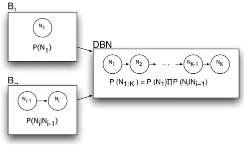
In the chord-recognition task, attribute and context variables can range from chord, key, meter, and any other variables of interest. DBNs extend the capability of first-order Markov Models increasing the number of musical re-lationships and hierarchies that can be tracked. This renders it particularly suited to model musical systems that include lots of interconnected variables. A DBN is defined to be a pair,(B1, B→), where B1 is a BN which defines

the prior P (Z1), and B→ is a two-slice temporal Bayes net (2TBN) which

definesP (Zi|Zi−1) by means of a DAG that factors as follows:

P (Zi|Zi−1) = K

Y

i=1

P (Z_ij_{|P arents(Z}_ij)). (3.39) where Z_ij indicates the Zj _{variable at time index} _{i. The resulting joint}

distribution is given by:

P (Z1:K) = K Y i=1 J Y j=1 P (Z_ij_{|P arents(Z}_ij)). (3.40) Building a DBN that include unobserved hidden states is straightforward. We only need to add the nodes and create the dependencies. Model specifi-cation is accomplished by specifying probability distributions inB1 andB→,

as in HMMs.

There are many standard inference types [32]. The one we will use is called offline smoothing because our system will have access to all the observations.

(54)

N1 Ni-1 Ni N1 N2 . . . NK-1 NK

B

_→

B

₁

DBN

P(N1) P(Ni|Ni-1) P (N1:K ) = P (N1)∏P (Ni|Ni−1)

Figure 3.12: Construction of a simple Dynamic Bayesian network, starting from the prior slice and tiling the 2TBN over time.

It is based on a 2 pass forward filtering-backward smoothing strategy, which is not discussed here because it is beyond the scope of this thesis.

(55)

Chapter 4

System Overview

In this chapter we will review the main components of our system. The first section is devoted to the beat-tracker subsystem. In the second section we will give an overview of the chord-recognition subsystem. Finally we will explain the three novel harmony-based features and the ideas behind them.

4.1 Beat tracking system

In this section we review in full detail every building block of the beat track-ing system (Fig. 4.2).

Starting from the audio signal s(n), we first compute the STFT and ex-tract the onset detection functionη(m). Periodicities in η(m) are estimated and stored inτ (m) by the tempo estimation block. Starting from η(m) and τ (m) the beat tracking stage extract the beat times b(i). These are exploited by the downbeat extraction stages, which extract downbeats db(k) among beats.

4.1.1 Onset strength envelope

The first step in computing the onset strength envelope is taking the short-Time Fourier Transform (STFT) of the signal. Starting from a stereo signal we first average the two channels to achieve a mono signal s(n), then the STFT is computed with window length ofN = 1024 samples and overlap of 50% (h = 512) obtaining a time-resolution of 11.6 ms: Sk(m) = ∞ X n=−∞ s(n)w(mh_{− n)e}−j2πk/N (4.1) 35

(56)

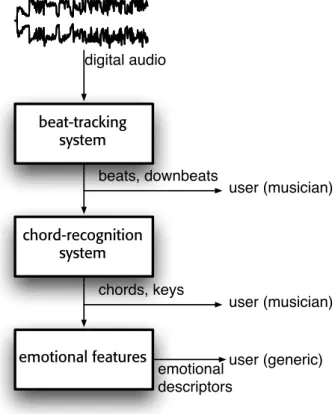
beat-tracking system chord-recognition system emotional features digital audio beats, downbeats chords, keys emotional descriptors user (musician) user (musician) user (generic)

Figure 4.1: The blocks that constitutes our system. Three types of information are extracted starting from digital audio. Rhythmic information is extracted by our beat tracker. Harmony-related information is extracted by our chord-recognition subsystem. These information are middle level features and are addressed to musically trained users. Harmony-related features are then extracted starting from key and chord information, and is addressed to a generic user (no training needed).

(57)

4.1. Beat tracking system 37

Tempo estimation

Rhythmogram Tempo path

Beat tracking

States reduction Beat sequence (Multipath) Onset detection η(m) η(m) τ(m) STFT Sk(m) s(n) b(i) Features extraction Time-signature estimation Downbeat tracking D(i) D(i) TS(i) beat level measure level db(k)

(58)

A basic energy-based onset detection function can be constructed by differ-entiating consecutive magnitude frames:

δSk(m) = N

X

k=1

|Sk(m)| − |Sk(m− 1)| (4.2)

This exploits the fact that energy bursts are often related to transients. Ne-glecting the phase information, however, results in great performance losses when dealing with non-percussive signals, where soft "tonal" onsets are re-lated to abrupt phase shifts in a frequency component. To track phase rere-lated onsets, we consider the phase shift difference between successive frames. This consists in taking the second derivative of unwrapped phaseψk(m) and then

wrapping again into the [−π, π] interval:

dψ,k(m) = wrap[(ψk(m)− ψk(m− 1)) − (ψk(m− 1) − ψk(m− 2))]. (4.3)

As said, the onset detection computed through a combination of energy-based and phase-energy-based approaches performs better than using only one of them. Simultaneous analysis of both energy and phase-based approach is obtained through a computation in the complex domain. The combined equation is:

Γk(m) ={|Sk(m− 1)|2+|Sk(m)|2−

− 2|Sk(m− 1)||Sk(m− 1)| cos dψ,k(m)}1/2 (4.4)

And the detection functionη(m) (Fig. 4.3) is obtained by summing over the frequency bins. η(m) = K X k=1 Γk(m) (4.5)

η(m) is equal to the energy based onset function when dψ,k(m) = 0.

η(m) = K X k=1 {|Sk(m− 1)|2+|Sk(m)|2− 2|Sk(m− 1)||Sk(m− 1)|}1/2= = K X k=1 |Sk(m)| − |Sk(m− 1)| (4.6)

Before proceeding to next stage we remove leading and trailing zeros from η(m).

Automatic chord recognition based on the probabilistic modeling of diatonic modal harmony