2021-01-27T10:02:31Z
Acceptance in OA@INAF
þÿALMA [C i]3 P 1 3 P 0 Observations of NGC 6240: A Puzzling Molecular Outflow,
þÿand the Role of Outflows in the Global ± CO Factor of (U)LIRGs
Title
CICONE, CLAUDIA; SEVERGNINI, Paola; Papadopoulos, Padelis P.; Maiolino,
Roberto; Feruglio, Chiara; et al.
Authors
10.3847/1538-4357/aad32a
DOI
http://hdl.handle.net/20.500.12386/30026
Handle
THE ASTROPHYSICAL JOURNAL
Journal
863
ALMA
[C
I
]
3P
1–
3P
0
Observations of NGC 6240: A Puzzling Molecular Out
flow, and the
Role of Out
flows in the Global α
COFactor of
(U)LIRGs
Claudia Cicone1,15 , Paola Severgnini1, Padelis P. Papadopoulos2,3,4, Roberto Maiolino5,6, Chiara Feruglio7, Ezequiel Treister8 , George C. Privon9 , Zhi-yu Zhang10,11, Roberto Della Ceca1, Fabrizio Fiore12, Kevin Schawinski13 , and Jeff Wagg14
1INAF—Osservatorio Astronomico di Brera, Via Brera 28, I-20121 Milano, Italy;
2
Department of Physics, Section of Astrophysics, Astronomy and Mechanics, Aristotle University of Thessaloniki, Thessaloniki, Macedonia, 54124, Greece 3
Research Center for Astronomy, Academy of Athens, Soranou Efesiou 4, GR-115 27 Athens, Greece 4
School of Physics and Astronomy, Cardiff University, Queen’s Buildings, The Parade, Cardiff, CF24 3AA, UK 5
Cavendish Laboratory, University of Cambridge, 19 J. J. Thomson Ave., Cambridge CB3 0HE, UK 6
Kavli Institute of Cosmology Cambridge, Madingley Road, Cambridge CB3 0HA, UK 7
INAF—Osservatorio Astronomico di Trieste, via G.B. Tiepolo 11, I-34143 Trieste, Italy 8
Instituto de Astrofisica, Facultad de Fisica, Pontificia Universidad Catolica de Chile, Casilla 306, Santiago 22, Chile 9
Department of Astronomy, University of Florida, 211 Bryant Space Sciences Center, Gainesville, 32611 FL, USA 10
European Southern Observatory, Karl-Schwarzschild-Strae 2, D-85748 Garching, Germany 11
Institute for Astronomy, University of Edinburgh, Royal Observatory, Blackford Hill, Edinburgh EH9 3HJ, UK 12INAF—Osservatorio Astronomico di Roma, via Frascati 33, I-00078 Monteporzio Catone, Italy 13
Institute for Particle Physics and Astrophysics, ETH Zurich, Wolfgang-Pauli-Str. 27, CH-8093 Zurich, Switzerland 14SKA Organisation, Lower Withington Macclesfield, Cheshire SK11 9DL, UK
Received 2018 April 7; revised 2018 June 29; accepted 2018 July 11; published 2018 August 20
Abstract
We present Atacama large millimeter/submillimeter array (ALMA) and compact array (ACA) [CI]3P - P
1 3 0([CI]
(1–0)) observations of NGC6240, which we combine with ALMA CO(2–1)and IRAM Plateau de Bure Interferometer CO(1–0)data to study the physical properties of the massive molecular (H2) outflow. We discover that the receding and approaching sides of the H2outflow, aligned east–west, exceed 10 kpc in their total extent. High resolution( 0. 24) [CI](1–0)line images surprisingly reveal that the outflow emission peaks between the two
active galactic nuclei (AGNs), rather than on either of the two, and that it dominates the velocity field in this nuclear region. We combine the[CI](1–0)and CO(1–0)data to constrain the CO-to-H2conversion factor(aCO) in
the outflow, which is on average 2.11.2M(K km s-1pc2)-1. We estimate that 60±20% of the
total H2 gas reservoir of NGC6240 is entrained in the outflow, for a resulting mass-loss rate of
= - º
˙
Mout 2500 1200M yr 1 50 30 SFR. These energetics rule out a solely star formation-driven wind, but the puzzling morphology challenges a classic radiative-mode AGN feedback scenario. For the quiescent gas, we compute aá COñ =3.21.8M(K km s-1pc2)-1, which is at least twice the value commonly employed for
(ultra) luminous infrared galaxies ((U)LIRGs). We observe a tentative trend of increasingr21º ¢LCO 2 1( - ) LCO 1 0¢ ( -) ratios with velocity dispersion and measure r21>1 in the outflow, whereas r21;1 in the quiescent gas. We propose that molecular outflows are the location of the warmer, strongly unbound phase that partially reduces the opacity of the CO lines in(U)LIRGs, hence driving down their global aCOand increasing their r21values. Key words: galaxies: active– galaxies: evolution – galaxies: individual (NGC 6240) – galaxies: ISM – submillimeter: ISM
1. Introduction
Massive(Mmol>108Me) and extended (r1 kpc) outflows of cold and dense molecular(H2) gas have been discovered in a large number of starbursts and active galactic nuclei (AGNs) (Turner1985; Nakai et al.1987; Sakamoto et al.2006; Feruglio et al.2010,2013a,2017; Fischer et al.2010; Alatalo et al.2011; Sturm et al. 2011; Dasyra & Combes 2012; Combes et al.
2013; Morganti et al. 2013; Spoon et al. 2013; Veilleux et al.
2013; Cicone et al. 2014; García-Burillo et al. 2014, 2015; Zschaechner et al. 2016; Carniani et al. 2017; Barcos-Muñoz et al. 2018; Fluetsch et al. 2018; Gowardhan et al. 2018).
Although so far limited mostly to local(ultra) luminous infrared galaxies ([U]LIRGs), these observations indicate that the mass-loss rates of H2gas are higher compared to the ionized gas phase participating in the outflows (Carniani et al. 2015; Fiore et al. 2017). Therefore, molecular outflows, by displacing and
perhaps removing the fuel available for star formation, can have a
strong impact on galaxy evolution. More luminous AGNs host more powerful H2winds, suggesting a direct link between the two (Cicone et al.2014).
The presence of massive amounts of cold and dense H2gas outflowing at v1000 km s−1across kpc scales in galaxies is itself puzzling. A significant theoretical effort has gone into reproducing the properties of multiphase outflows in the context of AGN feedback models (Cicone et al. 2018). In
one of the AGN radiative-mode scenarios, the outflows result from the interaction of fast highly ionized winds launched from the pc-scales with the kpc-scale interstellar medium (ISM), which occurs through a “blast-wave” mechanism (Silk & Rees 1998; King 2010; Faucher-Giguère & Quataert 2012; Zubovas & King 2012; Costa et al. 2014; Gaspari & Sa̧dowski 2017; Biernacki & Teyssier 2018). In this picture,
because molecular clouds overtaken by a hot and fast wind are quickly shredded (Brüggen & Scannapieco 2016), it is
more likely that the high-velocity H2 gas forms directly within the outflow, by cooling out of the warmer gas (Zubovas & King 2014; Costa et al.2015; Nims et al. 2015;
© 2018. The American Astronomical Society. All rights reserved.
15
Thompson et al.2016; Richings & Faucher-Giguère2018). An
alternative scenario, not requiring shockwaves, is the direct acceleration of the molecular ISM by radiation pressure on dust (Ishibashi & Fabian 2015; Thompson et al. 2015; Costa et al.2018). This mechanism is most efficient in AGNs deeply
embedded in a highly IR optically thick medium, such as local (U)LIRGs.
In order to advance our theoretical understanding of galactic-scale molecular outflows, we need to place more accurate constraints on their energetics. Indeed, most current H2outflow mass estimates are based on a single molecular gas tracer(CO or OH), implying uncertainties of up to one order of magnitude (Veilleux et al.2017; Cicone et al.2018). The luminosity of the
CO(1–0)line, which is optically thick in typical conditions of molecular clouds, can be converted into H2 mass through an CO(1–0)-to-H2conversion factor (aCO) calibrated using known
sources and dependent on the physical state of the gas. For the molecular ISM of isolated (or only slightly perturbed) disk galaxies like the Milky Way, the conventional aCOis
-
-( )
M
4.3 K km s 1pc2 1 (Bolatto et al. 2013). Instead, for
merger-driven starbursts like most (U)LIRGs, which are characterized by a more turbulent and excited ISM, a lower aCOof ~0.6 1.0– M(K km s-1pc2)-1is often adopted(Downes
& Solomon1998; Yao et al.2003; Israel et al.2015). Such low
aCOvalues have been ascribed to the existence, in the inner
regions of these mergers, of a warm and turbulent “envelope” phase of H2gas, not contained in self-gravitating clouds(Aalto et al. 1995). However, some recent analyses of the CO spectral
line energy distributions (SLEDs) including high-J (3) transitions suggest that near-Galactic aCOvalues are also possible
for(U)LIRGs, especially when a significant H2gas fraction is in dense, gravitationally bound states(Papadopoulos et al.2012a).
Dust-based ISM mass measurements also deliver galactic-type aCOfactors for (U)LIRGs, although they depend on the
under-lying assumptions used to calibrate the conversion (Scoville et al.2016).
Molecular outflows can be significantly fainter than the quiescent ISM, and so multi-transition observations aimed at estimating their aCOare particularly challenging. Dasyra et al.
(2016) and more recently Oosterloo et al. (2017), for the
radio-jet driven outflow in IC5063, derived a low optically thin aCOof ~0.3M(K km s-1pc2)-1, in line with theoretical
predictions by Richings and Faucher-Giguère (2018). On the
other hand, for the starburst-driven M82 outflow, Leroy et al. (2015) calculated16 a2 1CO- =1 2.5– M(K km s-1pc2)-1. The
detection of high density gas in the starburst-driven outflow of NGC253 would also favor an aCOhigher than the optically
thin value(Walter et al.2017), and a similar conclusion may be
reached for the outflow in Mrk231, found to entrain a substantial amount of dense H2gas(Aalto et al. 2012,2015; Cicone et al.2012; Lindberg et al.2016).
An alternative method for measuring the molecular gas mass, independent of the aCOfactor, is through a tracer such as
the3P - P
1 3 0transition of neutral atomic carbon(hereafter [CI]
(1–0)). This line, optically thin in most cases, has an easier partition function than molecules, and excitation requirements similar to CO(1–0).17 More importantly, [CI] is expected
to be fully coexisting with H2 (Papadopoulos et al. 2004; Papadopoulos & Greve 2004). Therefore, by combining the
information from CO(1–0)and [CI](1–0),it is possible to
derive an estimate of the aCOvalue. Similar to any optically
thin species used to trace H2(e.g., dust, 13
CO), converting the [CI](1–0)line flux into a mass measurement is plagued by the
unavoidable uncertainty on its abundance. However, in this regard, recent calculations found not only that the average [C/H2] abundance in molecular clouds is more robust than that of molecules such as CO, but also that[CI] can even trace the
H2gas where CO has been severely depleted by cosmic rays (CRs, Bisbas et al.2015,2017).
In this work we use new Atacama large millimeter/ submillimeter array (ALMA) and Atacama compact array (ACA) observations of the [CI](1–0)line in NGC6240 to
constrain the physical properties of its molecular outflow. NGC6240 is a merging LIRG hosting two AGNs with quasar-like luminosities(Puccetti et al.2016). The presence of
a molecular outflow was suggested by van der Werf et al. (1993), based on the detection of high-velocity wings of the
ro-vibrational H2 v=1–0 S(1)2.12 μm line and by Iono et al.(2007) based on the CO(3–2) kinematics, and it was later
confirmed by Feruglio et al. (2013a) using IRAM PdBI CO
(1–0)observations. This is one of the first interferometric [CI](1–0)observations of a local galaxy (see also Krips
et al.2016) and, to our knowledge, the first spatially resolved
[CI](1–0)observation of a molecular outflow in a quasar.
Probing the capability of [CI](1–0)to image molecular
outflows is crucial: besides being an alternative H2 tracer independent of the aCOfactor, [CI](1–0)is also sensitive to
CO-poor gas, which may be an important component of molecular outflows exposed to strong far-ultraviolet (UV) fields (Wolfire et al. 2010) or CR fluxes (Bisbas
et al. 2015, 2017; Krips et al. 2016; González-Alfonso et al. 2018). Moreover, testing [CI](1–0)as a sensitive
molecular probe in a local and well-studied galaxy such as NGC6240 has a great legacy value for studies at z>2, where the [CI] lines are very valuable tracers of the bulk of
the molecular gas accessible with ALMA(Zhang et al.2016).
The paper is organized as follows. In Section2we describe the data. In Section3.1we present the CO(1–0), CO(2–1), and [CI]
(1–0)outflow maps and the [CI](1–0)line moment maps. In
Sections3.2–3.3 we identify the outflowing components of the molecular line emission and derive the aCOand r21 values separately for the quiescent ISM and the outflow. The outflow energetics are constrained in Section3.4. In Section3.5we study the variations of aCOand r21as a function of svand distance of the different spectral components from the nucleus. Ourfindings are discussed in Section 4 and summarized in Section 5. Throughout the paper, we adopt a standardΛCDM cosmological model with H0=67.8 km s−1Mpc−1,ΩΛ=0.692, ΩM=0.308 (Planck Collaboration et al.2016). At the distance of NGC6240
(redshift z=0.02448, luminosity distance DL=110.3 Mpc), the physical scale is 0.509 kpcarcsec−1. Uncertainties correspond to 1σstatistical errors. The units of aCO[M(K km s-1pc2) ]-1 are
sometimes omitted.
2. Observations
The Band8 observations of the [CI](1–0)(n[restCI]=492.16065 GHz) emission line in NGC6240 were carried out in 2016 May with the 12 m diameter antennas of ALMA, and in 2016 August with the 7 m diameter antennas of the Atacama Compact Array
16By using the CO(2–1)transition. 17
CO(1–0)and [CI](1–0)are similar in critical density, but E10/kb=5.5 K for CO and 23 K for [CI]; however, as long as most of the H2 gas has Tk>15–20 K, as expected, the E/kbdifference between the two lines makes no real excitation difference in the level population(Papadopoulos et al.2004).
(ACA) as part of our Cycle3 programme 2015.1.00717.S (PI: Cicone). The ALMA observations were effectuated in a compact configuration with 40 antennas (minimum and maximum baselines, bmin=15 m, bmax=640 m), yielding an angular resolution (AR) of 0. 24 and a maximum recoverable scale (MRS) of 2. 48. Only one of the two planned 0.7-hour-long scheduling blocks was executed, and the total on-source time was 0.12 hours. The PWV was 0.65 mm, and the average system temperature was Tsys=612 K. The ACA observations were performed using nine antennas with bmin=9 m and bmax=45 m, resulting in AR= 2. 4 and MRS=14 . The total ACA observing time was 3.5 hours, with 0.7 hours on source. The average PWV and Tsys were 0.7 mm and 550 K, respectively. J1751+0939 and Titan were used for flux calibration, J1924-2914 for bandpass calibration, and J1658 +0741 and J1651+0129 for phase calibration.
We employed the same spectral setup for the ALMA and the ACA observations. Based on previous CO(1–0)observations of NGC6240 (Feruglio et al. 2013a, 2013b), and on the
knowledge of the concurrence of the [CI](1–0)and
CO(1–0)emissions, we expected the [CI](1–0)line to be
significantly broad (full width at zero intensity, FWZI > 1000 km s−1). Therefore, to recover both the broad [CI]
(1–0)line and its adjacent continuum, we placed two spectral windows at a distance of 1.8 GHz, overlapping by 75MHz in their central 1.875 GHz wide full sensitivity part, yielding a total bandwidth of 3.675 GHz (2293 km s−1) centered at n[obs]=480.40045 GHz
CI .
After calibrating separately the ALMA and ACA data sets with the respective scripts delivered to the PI, we fit and subtracted the continuum in the uv plane. This was done through the CASA18task uvcontsub, by using a zeroth-order polynomial for the fit, and by estimating the continuum emission in the following line-free frequency ranges:
n
< [ ]<
478.568 obs GHz 478.988 and 481.517<νobs[GHz] < 482.230. The line visibilities were then deconvolved using clean with Briggs weighting and robust parameter equal to 0.5. A spectral binning of Δν=9.77 MHz (6 km s−1) was applied, and the cleaning masks were chosen interactively. In order to improve the image reconstruction, following the strategy adopted by Hacar et al. (2018), we used the cleaned
ACA data cube corrected for primary beam as a source model to initialize the deconvolution of the ALMA line visibilities (parameter “modelimage” in clean). The synthesized beams of the resulting ACA and ALMA image data cubes are 4. 55 ´ 2. 98 (PA=−53°.57) and 0. 29´ 0. 24 (PA= 113°.18), respectively. In addition, a lower resolution ALMA [CI](1–0)line data cube was produced by applying a tapering
(outer taper of 1. 4), which resulted in a synthesized beam of
´
1. 28 1. 02 (PA=77°.49). Primary beam correction was applied to all data sets. We checked the accuracy of the ALMA and ACA relative flux scales by comparing the flux on the overlapping spatial scales between the two arrays, and found that they are consistent within the Band8 calibration uncertainty of 15%.
As a last step, in order to maximize the uv coverage and the sensitivity to any extended structure possiblyfiltered out by the ALMA data, we combined the(tapered and non) ALMA image data cubes with the ACA one using the task feather. For a detailed explanation of feather, we refer the reader to the
CASA cookbook.19The same steps were used to produce all the interferometric maps shown in this paper: (1) clean of ACA visibilities followed by primary beam correction, (2) clean of ALMA visibilities by using the ACA images as a source model followed by primary beam correction, and (3) feather of the ACA and ALMA images. The resulting ACA+ALMA merged images inherit the synthesized beam and cell size(the latter set equal to 0. 01 and 0. 2, respectively, for the higher and lower resolution data) of the corresponding input ALMA images. At the phase tracking center (central beam), the 1σsensitivities to line detection, calculated using the line-free spectral channels, are 1.4 mJy beam−1 and 5 mJy beam−1 per dv=50 km s−1 spectral channel, respec-tively, for the higher and lower resolution[CI](1–0)line data
cubes. The sensitivity decreases slightly with distance from the phase center. At a radius of 5″, the [CI](1–0)line sensitivities
per dv=50 km s−1 spectral channel are 3.3 mJy beam−1 and 5.5 mJy beam−1.
In this paper we make use of the IRAM PdBI CO(1–0)data previously presented by Feruglio et al.(2013a,2013b). The CO
(1–0)line image data cube used in this analysis has a synthesized beam of 1. 42´ 1. 00 (PA=56°.89) and a cell size of 0 2. The CO(1–0)1σline sensitivity per dv= 50 km s−1 spectral channel is 0.6 mJy beam−1 at the phase center, and 0.65 mJy beam−1at a 5 radius.
Our analysis also includes ALMA Band 6 (programme 2015.1.00370.S, PI: Treister) snapshot (1 minute on source) observations of NGC6240 targeting the CO(2–1)transition, which were performed in 2016 January (PWV=1.2 mm) using the compact configuration (AR= 1. 2, MRS =10). These observations were executed in support of the long baseline campaign carried out by E. Treister et al. (2018, in preparation). We calibrated the data using the script for PI, estimated the continuum from the line-free spectral ranges (224.106<νobs [GHz]<224.279 and 225.780< νobs[GHz] < 225.971), and subtracted it in the uv plane. We deconvolved the line visibilities using clean with Briggs weighting(robust=0.5) and applied a correction for primary beam. Thefinal CO(2–1)cleaned data cube has a synthesized beam of 1. 54´ 0. 92 (PA=60°.59) and a cell size of 0 2. The 1σ CO(2–1)line sensitivity per dv=50 km s−1channel is 0.80 mJy beam−1at the phase center and 1mJy beam−1at a 5″ radius.
In the analysis that follows, the comparison between the CO (1–0), CO(2–1), and [CI](1–0)line tracers in the molecular
outflow of NGC6240 will be done by using the lower resolution ALMA+ACA [CI](1–0)data cube, which matches
in AR (~ 1. 2) the IRAM PdBI CO(1–0)and ALMA CO (2–1)data. Unless specified, quoted errors include the systematic uncertainties on the measured fluxes due to flux calibration, which are 10% for the IRAM PdBI CO(1–0)and ALMA CO(2–1)data, and 15% for the ALMA [CI](1–0)line
observations. We report the presence of some negative artifacts, especially in the cleaned CO(1–0)and CO(2–1)data cubes. These are due to the interferometric nature of the observations, which does not allow to properly recover all the faint extended emission in a source with a very bright central peak emission such as NGC6240. However, the negative features lie mostly outside the region probed by our analysis, and they are not expected to significantly affect our flux recovery, since the total
18
CO(1–0)and CO(2–1)line fluxes are consistent with previous single-dish measurements (Costagliola et al. 2011; Papadopoulos et al. 2012b). Our total [CI](1–0)line flux is
higher than that recovered by Papadopoulos and Greve (2004) by using the James Clerk Maxwell telescope (JCMT,
FWHMbeam=10), but lower by 34±15% than the flux measured by the Herschel Space Observatory (Papadopoulos et al. 2014). This indicates that some faint extended emission
has been resolved out and/or that there is additional [CI]
(1–0)line emission outside the field of view of our observations.
3. Data Analysis and Results
3.1. Morphology of the Extended Molecular Outflow and Its Launch Region
With the aim of investigating the extent and morphology of the outflow, we produced interferometric maps of the CO(1–0), CO(2–1), and [CI](1–0)high-velocity emissions. The maps,
shown in Figures1(a)–(c), were generated by merging together
and imaging the uv visibilities corresponding to the blue- and redshifted wings of the molecular lines, integrated respectively within vä(−650, −200) km s−1 and v ä(250, 800) km s−1. These are the velocity ranges that, following from the identification of the outflow components performed in Section 3.3 (and further discussed in Section 4.1 and
AppendixB), are completely dominated by the emission from
outflowing gas. The data displayed in panels (a)–(c) have a matched spatial resolution equal to ~ 1. 2(details in Section2).
Panels(d), (e) of Figure1show the maps of the blue and red [CI](1–0)line wings at the native spatial resolution of the
ALMA Band 8 observations( 0. 24, Section2).
The extended(>5 kpc) components of the outflow are best seen in Figures 1(a)–(c), whereas panels (d), (e) provide a
zoomed view of the molecular wind in the inner 1–2 kpc. The bulk of the outflow extends eastward of the two AGNs, as already pointed out in the previous analysis of the CO (1–0)data done by Feruglio et al. (2013a). In addition, we
identify for thefirst time a western extension of the molecular outflow, roughly aligned along the same east–west axis as the eastern component. At the sensitivity allowed by our data, we detect at a S/N > 5 CO emission features associated with the outflow up to a maximum distance of 13. 3(6.8 kpc) and 7. 2 (3.7 kpc) from the nucleus, respectively, in the east and west directions(Figure1(a)–(c)). The [CI](1–0)map in Figure1(c)
shows extended structures similar to CO, although the limited field of view of the Band8 observations does not allow us to probe emission beyond a radius of ~ 7. 5.
Feruglio et al. (2013a) hinted at the possibility that the
redshifted CO detected in NGC6240 could be involved in the feedback process, but did not explicitly ascribe it to the outflow because of the smaller spatial extent of the red wing with
Figure 1.Extended NGC6240 outflow observed using different molecular gas tracers. The outflow emission, integrated within vä(−650, −200) km s−1(blue wing) and vä(250, 800) km s−1(red wing) and combined together, is shown in the maps (a)–(c), respectively, for the CO(1–0), CO(2–1), and [CI](1–0)transitions. The
three maps have matched spatial resolution(~ 1. 2, details in Section2). Contours correspond to (−3σ, 3σ, 6σ, 12σ, 24σ, 48σ, 150σ) with 1σ=0.14 mJy beam−1in panel(a); (−3σ, 3σ, 6σ, 24σ, 48σ, 200σ, 400σ) with 1σ=0.23 mJy beam−1in panel(b); (−3σ, 3σ, 6σ, 12σ, 24σ, 48σ) with 1σ=1.23 mJy beam−1in panel(c). Panels(d) and (e) show the maps of the [CI](1–0)blue and red wings at the original spatial resolution of the ALMA Band8 data ( 0. 24, details in Section2). Contours
correspond to(−3σ, 3σ, 6σ, 12σ, 18σ, 20σ) with 1σ=1.1 mJy beam−1in panel(d) and 1σ=1 mJy beam−1in panel(e). The black crosses indicate the VLBI positions of the AGNs from Hagiwara et al.(2011). The synthesized beams are shown at the bottom-left of each map. The grid encompassing the central ´ 12 6 region and employed in the spectral analyses presented in Sections3.2and3.3is drawn in panel(a).
respect to the blue wing. In Figure 2we directly compare the blue and red line wings using the ALMA CO(2–1)data. Based on their close spatial correspondence, whereby the red wing overlaps with the blue one across more than 7 kpc along the east–west direction, we conclude that both the redshifted and blueshifted velocity components trace the same massive molecular outflow. It follows that the eastern and western sides of the outflow are detected in both their approaching and receding components. At east, the blueshifted emission is brighter than the redshifted one and dominant beyond a 3.5 kpc radius.
The ALMA [CI](1–0)data can be used to identify with high
precision the location of the inner portion of the molecular outflow. Figures 1(d), (e) clearly show that the red wing peaks in the
midpoint between the two AGNs, and that the blue wing has a maximum of intensity closer to the southern AGN, as already noted by Feruglio et al.(2013a). However, these data reveal for the
first time that neither the blue nor the redshifted high-velocity [CI]
(1–0)emissions peak exactly at the AGN positions. The blue wing has a maximum of intensity at R.A.(J2000)=16:52:58.8946± 0.0011s, decl.(J2000)=+02.24.03.52 0. 02, offset by 0. 18
0. 02 to the north-east with respect to the southern AGN. The red wing instead peaks at R.A.(J2000)=16:52:58.9224±0.0007s, decl.(J2000)=+02.24.04.0158 0. 007 (i.e., at an approxi-mately equal distance of 0. 8 from the two AGNs ). The [CI]
(1–0)red and blue wing peaks are separated by 0. 65 0. 02. This separation is consistent with the distance between the CO(2–1)peaks reported by Tacconi et al. (1999), although in that
work they were interpreted as the signature of a rotating molecular gas disk.
The presence of such nuclear rotating H2structure has been largely debated in the literature, especially due to the very high CO velocity dispersion in this region(σ>300 km s−1), and to the mismatch between the dynamics of H2 gas and stars (Gerssen et al. 2004; Engel et al. 2010). Following
Tacconi et al. (1999) and Bryant and Scoville (1999), if a
rotating disk is present, its signature should appear at lower projected velocities than those imaged in Figures1(d), (e). In
Figure 3 we show the high resolution intensity-weighted moment maps of the [CI](1–0)line emission within -200<
<
-[ ]
v km s 1 250. The velocity field does not exhibit the characteristic butterfly pattern of a rotating disk, but it presents a highly asymmetric gradient whereby blueshifted velocities dominate the southern emission, whereas near-systemic and redshifted velocities characterize the northern emission. These features in the velocityfield are correlated in both velocity and position with the high-velocity wings (Figures 1(d), (e)).
Furthermore, the right panel of Figure3shows that the velocity dispersion is uniform ( 50 sv[km s-1]80) throughout the entire source and enhanced (σv 100 km s−1) in a central hourglass-shaped structure extending east–west, which is the same direction of expansion of the larger-scale outflow. This structure has a high-σvpeak withσv 150 km s−1to the east and another possible peak to the west with σv 130 km s−1. Such high-σv points coincide with the blue and redshifted velocity peaks detected in the moment1 map. Therefore, based on Figure 3, we conclude that the molecular gas emission between the two AGNs is dominated by a nuclear outflow expanding east–west and connected to the larger-scale outflow shown in Figure 1. The regions of enhanced turbulence may represent the places where the outflow opening angle widens up, hence increasing the line of sight velocity dispersion and velocity of the molecular gas.
3.2. The aCOValues Estimated from the Integrated Spectra: A
Reference for Unresolved Studies
Figure4shows the CO(1–0), CO(2–1), and [CI](1–0)spectra
extracted from the12 ´ 6 -size rectangular aperture reported in Figure 1(a), encompassing both the nucleus and the extended
molecular outflow of NGC6240. The analysis of these integrated spectra, described later, is aimed at deriving a source-averaged aCOfor the quiescent and outflowing molecular ISM in
NGC6240. Such analysis is included here because it can be useful as a reference for unresolved observations (e.g., high redshift analogues of this merger). We stress, however, that the quality of our data, the proximity of the source, and its large spatial extent allow us to perform a much more detailed, spatially resolved analysis. The latter will be presented in Section3.3and delivers the most reliable aCOvalues for the outflow and the
quiescent gas.
The spectra in Figure4 were fitted simultaneously using two Gaussians to account for the narrow core and broad wings of the emission lines, by constraining the central velocity(v) and velocity dispersion(σv) of each Gaussian to be equal in the three transitions. Table 1 reports the best fit results and the corresponding line luminosities calculated from the integrated fluxes following Solomon et al. (1997). The [CI](1–0)line luminosities listed in
Table1are employed to measure the molecular gas mass(Mmol, including the contribution from helium) associated with the narrow and broad line components. The expression for local thermo-dynamic equilibrium (LTE; i.e., uniform Tex) and optically thin emission (t[CI]( – )1 0 1), assuming a negligible background
(CMB temperature, TCMB=Tex) and the Rayleigh–Jeans
Figure 2.Comparison between the CO(2–1)blue and red wing emissions in NGC6240. For visualization purposes, only positive contours starting from 5σare shown, with 1σ=0.33 mJy beam−1for the blue wing(blue contours) and 1σ=0.3 mJy beam−1for the red wing(red contours). The corresponding interferometric maps including negative contours are displayed in AppendixA
approximation(hν[CI](1–0)=kTex), is = + + ¢ - -- - [ ] ( · ) · · ( )· · [ ] ( ) [ ] [ ] [ ] [ ]( – ) M M X e e e L 4.31 10 1 3 5 K km s pc , 1 T T T mol 5 C1 23.6 K 62.5 K 23.6 K C I 1 0 1 2 I ex ex ex
where XCI is the [CI H2] abundance ratio and Tex is the excitation temperature of the gas(see detailed explanations by Papadopoulos et al. 2004 and Mangum & Shirley2015). We
adopt Tex=30 K and XCI=(3.0±1.5)×10−5, which
are appropriate for (U)LIRGs (Weiß et al. 2003, 2005; Papadopoulos et al. 2004; Walter et al. 2011; Jiao et al.
2017). These assumptions will be further discussed in
Section 4.1.2.
By defining a [CI](1–0)-to-H2 conversion factor (α[CI])
in analogy with the commonly employed aCOfactor
(Bolatto et al.2013), Equation (1) resolves into
a a º ¢ = -- - [ ] [ ] [ ( ) ] ( ) [ ] [ ] [ ] M M L M K km s pc with 9.43 K km s pc . 2 mol C C 1 2 C 1 2 1 I I I
Using the values in Table1and Equation(2), we obtain a total
molecular gas mass of Mmol=(1.50.8) ·1010 M, of
which (53) ·109 M is in the narrow component, and
(10 5) ·109 M in the broad wings. We then use these M mol
Figure 3.Intensity-weighted moment maps of the[CI](1–0)line emission in the merger nucleus. The maps were computed from the higher resolution ALMA+ACA
merged data cube(see Section2) by using the task immoments and by selecting the spectral range vä(−200, 250) km s−1. Contours correspond to[−100, −50, 0, 50, 100, 150] km s−1(moment 1, central panel) and [50, 80, 100, 110, 130, 170, 180] km s−1(moment 2, right panel).
Figure 4.Total CO(1–0), CO(2–1), and [CI](1–0)spectra extracted from a
´
12 6 -size rectangular region centered at R.A.=16:52:58.900, decl.=02.24.03.950, and displayed in Figure 1(a). The rms values per
spectral channel are 3.2mJy (δv=53 km s−1), 17mJy (δv=13 km s−1), and 78mJy (δv=49 km s−1), respectively, for CO(1–0), CO(2–1), and [CI](1–0).
The spectra were simultaneously fitted using two Gaussian functions (white dashed curves) tied to have the same velocity and width in all three transitions. The best fit results are reported in Table 1. The source-averaged r21 and aCOcalculated from this fit are listed in Table2.
Table 1
Results of the Simultaneous Fit to the Total Spectraa
CO(1–0) CO(2–1) [CI](1–0) Narrow component vb[km s−1] −9.1±1.0 −9.1±1.0 −9.1±1.0 sv[km s−1] 101.0±1.0 101.0±1.0 101.0±1.0 Speak[mJy] 211±4 1058±12 1360±70 òS dvv [Jy km s−1] 53.4±1.0 268±4 344±18 ¢ L [109K km s−1pc2] 1.55±0.03 1.94±0.03 0.55±0.03 Broad component vb[km s−1] 78.0±1.2 78.0±1.2 78.0±1.2 σv[km s−1] 264.4±1.0 264.4±1.0 264.4±1.0 Speak[mJy] 301±3 1458±12 1040±40 òS dvv [Jy km s−1] 199±2 966±9 690±30 L′ [109K km s−1pc2] 5.78±0.06 7.01±0.06 1.09±0.05 Total line òS dvv [Jy km s−1] 253±2 1234±10 1030±30 L′ [109K km s−1pc2] 7.33±0.07 8.96±0.07 1.64±0.05 Notes. a
The errors quoted in this table are purely statistical and do not include the absoluteflux calibration uncertainty.
bWe employ the optical Doppler definition. The fit allows for a global velocity shift of CO(2–1)and [CI](1–0)with respect to CO(1–0)to take into account the
different spectral binning. The best fit returns: vCO 2(-1)-vCO 1(-0)=10.2 0.9 km s−1andv[CI](1-0)-vCO 1(-0)= -184km s−1.
values to estimate aCO: a = ¢ - - [ ] ( ( – )[ ]) ( ) M M L K km s pc . 3 CO mol CO 1 0 1 2 1
The results are reported in thefirst three rows of Table2for the the total, narrow, and broad emissions in NGC6240. The so-derived aCOfactors differ between the narrow and broad line
components, being a factor of 1.8±0.5 lower in the latter.20In the narrow component, the aCOis significantly higher than the
typical (U)LIRG value. As mentioned in Section 1, higher aCOvalues become possible in (U)LIRGs if a significant
fraction of the mass is“hidden” in dense and bound H2clouds. This is probably the case of NGC6240, in which a large study using CO SLEDs from J=1–0 up to J=13–12 from the Herschel Space Observatory, as well as multi-J HCN, CS, and HCO+ line data from ground-based observatories, finds aCO
~ -
-
– M ( )
2 4 K km s 1pc2 1(Papadopoulos et al. 2014),
con-sistent with our estimates.
Table 2 lists also the CO(2–1)/CO(1–0)luminosity ratios, defined as
º ¢ ( - ) ¢ ( - ) ( )
r21 LCO 2 1 LCO 1 0. 4 Wefind r21as consistently∼1.2—hence higher than unity (at the 1.5σ level)—for both the narrow and broad Gaussian components. Since our total CO(1–0)and CO(2–1)fluxes are consistent with previous measurements(Costagliola et al.2011; Papadopoulos et al.2012b; Saito et al.2018), we exclude that
spatial filtering due to an incomplete uv coverage is significantly affecting the r21 values. As pointed out by Papadopoulos et al. (2012b), galaxy-averaged r21>1 values are not uncommon in(U)LIRGs and are indicative of extreme gas conditions. In this analysis of the integrated spectra, we derived r21>1 in both the broad and narrow components. However, as we will show in Sections3.3and3.5, the spatially resolved analysis will reveal that r211 values are typical of
the outflowing gas and in general of higher-σv components, while the“quiescent” ISM has r21∼1.
3.3. Spatially Resolved Analysis: The Average aCOof the
Quiescent and Outflowing Gas
The previous analysis(Section3.2) was based on the spectral fit
shown in Figure4, where we decomposed the total molecular line emission into a narrow and a broad Gaussian. In first approximation, these two spectral components can be respectively identified with the quiescent and outflowing molecular gas reservoirs of NGC6240. However, the superb S/N and spatial resolution of our data allow us to take this analysis one step further and refine the definition of quiescent and outflowing components. This is done by including the spatially resolved information provided by the interferometric data, as described later.
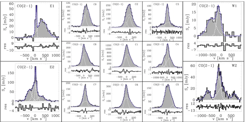
We divide the central 12 ´ 6 region employed in the previous analysis into a grid of 13 squared boxes and use them as apertures to extract the corresponding CO(1–0), CO(2–1), and [CI](1–0)spectra. As shown in Figure 1(a), the central
nine boxes have a size of 2 ´ 2 , while the external four boxes have a size of ´ 3 3 . The box spectra are presented in AppendixB(Figures 8–10).
For each box, the CO(1–0), CO(2–1), and [CI](1–0)spectra are
fitted simultaneously with a combination of Gaussian functions tied to have the same line centers and widths for all three transitions. In the fitting procedure, we minimize the number of spectral components required to reproduce the line profiles, up to a maximum of four Gaussians per box. The Gaussian functions employed by the simultaneous fit span a wide range in FWHM and velocity, shown in Figure5. The next step is to classify each of these components as“systemic” or “outflow.” In many local (U) LIRGs, molecular outflows can be traced through components whose kinematical and spatial features deviate from a rotating molecular structure(Cicone et al.2014; García-Burillo et al.2014).
However, in this source we do not detect any clear velocity gradient that may indicate the presence of a rotating molecular gas disk (Figure 3). Therefore, we adopt a different method and
identify as“quiescent” the gas probed by the spectral narrow line components that are detected throughout the entire source extent (Figures8–10). Our simultaneous fit to the CO(1–0), CO(2–1), and
Table 2 aCOand r21Valuesa aCO r21 - - [M (K km s 1pc2) ]1 Totalb 2.1±1.1 1.22±0.14
Totalbnarrow comp 3.3±1.8 1.25±0.18
Totalbbroad comp 1.8±0.9 1.21±0.17
Meancglobal 2.5±1.4 1.17±0.19
Meancsystemic comp 3.2±1.8 1.0±0.2
Meancoutflow comp 2.1±1.2 1.4±0.3
Notes. a
Quoted errors are dominated by systematic uncertainties(e.g., absolute flux calibration errors, error on XCI).
b
Calculated from the simultaneousfit to the total CO(1–0), CO(2–1), and [CI]
(1–0)spectra shown in Figure4, whose results are reported in Table1(details
in Section3.2).
c
Mean values calculated from the simultaneousfit to the CO(1–0), CO(2–1), and [CI](1–0)spectra extracted from the grid of 13 boxes shown in
Figure1(a), as explained in Section3.3. The corresponding spectralfits are shown in AppendixB(Figures8–10).
Figure 5.FWHM as a function of central velocity of all Gaussian components employed in the simultaneous fitting of the CO(1–0), CO(2–1), and [CI]
(1–0)box spectra. The blue dashed rectangle constrains the region of the parameter space that we ascribe to the“systemic” components.
20
In estimating the error on this ratio, we have ignored the systematic uncertainty on XCI, assuming it affects both aCOmeasurements in the same way.
[CI](1–0)spectra returns for these narrow components typical
FWHM and central velocities in the ranges:
FWHM<400 km s−1 and -200<v[km s-1]<250, consis-tent with what found by Feruglio et al. (2013b).21 Based on these results, we assume that all components with -200 <v[km s-1]<250 and FWHM < 400 km s−1 trace quiescent gas that is not involved in the outflow. These constraints correspond to the region of the FWHM-v parameter space delimited by the blue dashed lines in Figure 5. All components outside this rectangular area are classified as “outflow.” These assumptions are discussed in detail and validated in AppendixB, whereas more general considerations about our outflow identifica-tion method are reported in Secidentifica-tion4.1.1.
Using the results of the simultaneous fit, we measure, for each box and for each of the CO(1–0), CO(2–1), and [CI]
(1–0)transitions, the velocity-integrated fluxes apportioned in the“systemic” and “outflow” components. These are computed by summing the fluxes from the respectively classified Gaussian functions fitted to the molecular line profiles. For example, in the case of the central box (labeled as “C1” in Figures8–10), the simultaneous fit employs three Gaussians: a
narrow one classified as “systemic,” and two additional ones classified as “outflow.” The flux of the first Gaussian corresponds to the flux of the “systemic” component for this box, whereas the total “outflow” component flux is given by the sum of thefluxes of the other two Gaussians (the errors are added in quadrature).
The velocity-integrated fluxes (total, systemic, outflow) are then converted into line luminosities and, from these, the corresponding aCOand r21 can be derived by following the same steps as in Section 3.2 (Equations (2)–(4)). Table 2
(bottom three rows) lists the resulting mean values of aCOand
r21obtained from the analysis of all 13 boxes. In computing the mean, we only include the components detected at a S/N 3 in each of the transitions used to calculate aCOor r21—that is, CO(1–0)and [CI](1–0)for the former, and CO(1–0)and
CO(2–1)for the latter. The new aCOvalues derived for the
systemic and outflowing components, respectively equal to 3.2±1.8 and 2.1±1.2, are perfectly consistent with the previous analysis based on the integrated spectra. Instead, this new analysis delivers different ár21ñ values for the systemic
(1.0 ± 0.2) and outflowing component (1.4 ± 0.3), although still consistent if considering the associated uncertainties (dominated by the flux calibration errors).
By using the CO(1–0)line data and summing the contrib-ution from all boxes, including both the systemic and the outflowing components, we derive a total molecular gas mass of Mmoltot =(2.10.5)´1010 M. To compute the Mmol within each box we adopt, when available, the “global” aCOfactor estimated for that same box; otherwise, we use the
mean value of aCO=2.5±1.4.22 Compared with previous
works recovering the same amount of COflux, our new Mmol tot
estimate is higher than in Tacconi et al. (1999) and Feruglio
et al.(2013a), but consistent with Papadopoulos et al. (2014).
3.4. Molecular Outflow Properties
In this section we use the results of the spatially resolved spectral analysis presented in Section 3.3 to constrain the mass (Mout), mass-loss rate ( ˙Mout), kinetic power (1 2M˙outv2), and
momentum rate( ˙Moutv) of the molecular outflow. We first select the boxes in which an outflow component is detected in the CO (1–0)spectrum with S/N 3. As described in Section 3.3, the outflow component is defined as the sum of all Gaussian functions employed by the simultaneousfit that lie outside the rectangular region of the FWHM-v parameter space shown in Figure5. With this S/N 3 constraint, 12 boxes (that is, all except W1) are selected to have an outflow component in CO(1–0), and for each box,23we measure the following:
(i) The average outflow velocity (vout,i), equal to the mean of the (moduli of the) central velocities of the individual Gaussians classified as “outflow”
(ii) The molecular gas mass in outflow (Mout,i), calculated by multiplying the LCO 1 0¢ ( – ) of each outflow component by an appropriate aCO. In ten boxes, the outflow component
is detected with S/N 3 also in the [CI](1–0)transition;
hence for these boxes we can use their corresponding aCOfactor (see Section3.3). For the remaining two boxes
(E1 and W2), we adopt the galaxy-averaged outflow aCOof 2.1±1.2 (Table2).
(iii) The dynamical timescale of the outflow, defined as τdyn,i= Ri/vout,i, where Ri is the distance of the center of the box from R.A.=16:52:58.900, decl.=02.24.03.950. This definition cannot be applied to the central box (C1) because the so-estimated R would be zero, hence boosting the mass-loss rate to infinite. Therefore, for box C1, we conservatively assume that most of the outflow emission comes from a radius of 1 ; hence we set R=0.5 kpc. For all boxes, we assume the uncertainty on Ri to be 0. 6 (0.3 kpc), which is half a beam size.
(iv) The mass-loss rate ˙Mout,i, equal to Mout,i/τdyn,i All uncertainties are derived by error propagation.
The resulting total outflow mass and mass-loss rate, obtained by adding the contribution from all boxes, are respectively
=( )´
Mout 1.2 0.3 1010 M and dMout/dt=2500± 1200 M yr -1. As discussed in Appendix B, the largest
contribution to both ˙Mout and its uncertainty is given by the
central box. Indeed, box C1 has at the same time the highest estimated Moutand the smallest—and most uncertain—R, because the outflow is launched from within this region, likely close to the midpoint between the two AGNs, as suggested by Figures1(d), (e).
Similar to the mass-loss rate, we calculate the total kinetic power and momentum rate of the outflow by summing the contribution from all boxes with a CO(1–0)outflow component, and we obtain, respectively, 1 2M˙out outv2 º å 1 2M˙ v =(0.0330.019) L
i out, out,i 2 i AGN and vM˙outº
åi iv M˙out,i=(8050) LAGN c. If all the gas carried by the outflow escaped the system and the mass-loss continued at the current rate, the depletion timescale of the molecular gas reservoir in NGC6240 would be τdep=8±4 Myr. All the relevant numbers describing the properties of the source and of
21Feruglio et al. (2013b) analyzed the CO(1–0)spectra extracted from different positions within NGC6240 and found maximum velocity shift and FWHM of the narrow Gaussians of ∣vsysmax∣=824km s−1 and FWHMsysmax=380150 km s−1.
22
This was the case for the three boxes(labeled as “E1,” “W1,” and “W2” in Figures8–10) without a S/N 3 detection of [CI](1–0).
23
All quantities relevant to the individual boxes are identified by an index i=1, 12 (e.g., vout,i) in order to distinguish them from the corresponding galaxy-integrated quantities(e.g., vout).
the molecular outflow are reported in Table 3 and will be discussed in Section4.3in the context of feedback models.
Very stringent lower limits on the outflow energetics can be derived by assuming that its CO(1–0)emission is fully optically thin. For optically thin gas and Tex=30 K, the aCOfactor would
be∼0.34 (Bolatto et al.2013), and the outflow mass and mass-loss
rate would beMout =(1.980.09)´109 Mand dMout/dt= 430±160 M yr -1. However, we stress that the assumption of
fully optically thin CO(1–0)emission in the outflow is not supported by our data, which instead favor an aCOfactor for
outflowing gas that is intermediate between the optically thin and the optically thick values(for solar metallicities).
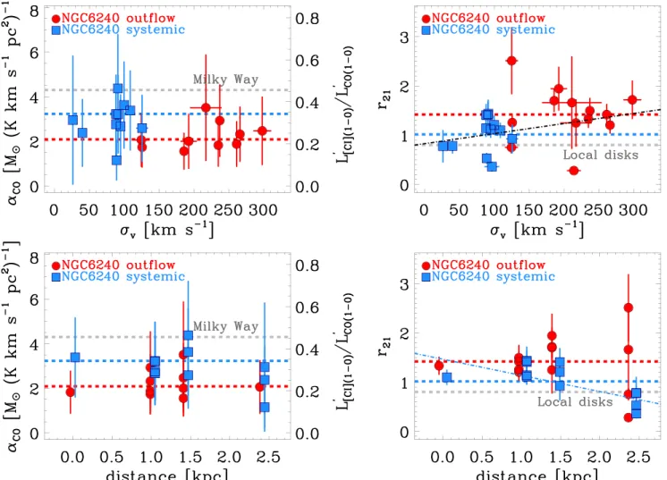
3.5. Physical Properties of Quiescent and Outflowing Gas Using the results of the spatially resolved analysis presented in Section3.3, we now study how the aCOand r21parameters vary as a function of velocity dispersion (σv) and projected distance(d) from the nucleus of NGC6240. The relevant plots are shown in Figure 6. To investigate possible statistical correlations, we conduct a Bayesian linear regression analysis of the relations in Figure 6, following Kelly(2007).24
The left panels of Figure6 do not indicate any statistically significant relation between aCOand either σv or d. Instead, they show that the aCOfactor is systematically higher—
although formally only at a significance of 1.2σ (Table2)—in
the quiescent gas than in the outflow, regardless of the velocity dispersion of the clouds, or of their position with respect to the merger nucleus. For the non-outflowing components, the aCOfactors are at least twice the so-called (U)LIRG value
(Downes & Solomon1998), and reach up to Galactic values.
This result is consistent with the multi-transition analysis by Papadopoulos et al.(2014), and is likely due to the state of the
dense gas phase that low-J CO lines alone cannot constrain, but which instead is accounted for when using [CI](1–0)as a
molecular mass tracer. Nevertheless, the outflowing H2gas has lower aCOvalues than the quiescent ISM. This is indeed
expected from the ISM physics behind aCOfor warm and
strongly unbound gas states(Papadopoulos et al.2012a)—that
is, the type of gas that we expect to be embedded in outflows. In particular, in the case that molecular outflows are ubiquitous in(U)LIRGs, as suggested by observations (Sturm et al.2011; Spoon et al.2013; Veilleux et al.2013; Cicone et al.2014), the
outflow may be the location of the diffuse and warm molecular gas phase that is not contained in self-gravitating cooler clouds —a sort of “intercloud” medium advocated by some of the previous analyses based solely on low-J CO, 13CO line observations (Aalto et al. 1995; Downes & Solomon 1998).
Furthermore, the flat trend between aCOand d observed in
Figure 6 does not support the hypothesis that the lower aCOvalues in (U)LIRGs are related to the collision of the
progenitors’ disks, since in this case we would naively expect the loweraCOclouds to be concentrated in the central regions
of the merger. The aCOvalues measured for the outflow
components are, however, significantly higher than the optically thin value, suggesting that not all of the outflowing material is diffuse and warm, but there may still be a significant amount of dense gas. These results are further discussed and contextualized in Section4.2.
The right panels of Figure 6 show a weak correlation between the r21andσv(correlation coefficient, ρ=0.4±0.2) and an anti-correlation with the distance, although only for the systemic/quiescent components (ρ=−0.7±0.2). The corresponding best fit relations, of the form r21=α+βx, plotted in Figure 6, have (α, β)=(0.8±0.2, 2.1±1.4× 10⁻³) for x=σv, and(α, β)=(1.5±0.2, −0.33±0.13) for x=d. The systemic ISM shows 0.8r211.4, whereas the outflow is characterized by higher ratios, with most compo-nents in the range 1.2r212.5, although we observe a large spread in r21values at d>2 kpc.
CO(2–1)/CO(1–0)luminosity ratios of r21∼0.8–1.0 are typically found in the molecular disks of normal spiral galaxies (Leroy et al. 2009) and are indicative of optically thick CO
emission with Tkin∼10–30 K (under LTE assumptions). Nevertheless, such low-J CO line ratios, in absence of additional transitions, are well-known to be highly degenerate tracers of the average gas physical conditions. Higher-J data of CO, molecules with larger dipole moment, and isotopologues can break such degeneracies. Such studies exist for NGC6240 (Greve et al. 2009; Meijerink et al 2013; Papadopoulos et al. 2014), and found extraordinary states for the molecular
gas, with average densities typically above 104cm−3 and temperatures Tkin∼30–100 K.
Table 3
Summary of Source and Outflow Properties Source properties m ( – ) LTIR 8 1000 m [erg s−1] 2.71×1045a LBol[erg s−1] 3.11×1045b LAGN[erg s−1] (1.1±0.4)×1045c αAGN≡LAGN/LBol 0.35±0.13 SFR[Myr−1] 46±9d Mmoltot [M ] (2.1±0.5)×1010e
Molecular outflow properties (estimated in Section3.4)
rmax[kpc] 2.4±0.3f ávoutñ[km s−1] 250±50g s áoutñ[km s−1] 220±20g t ádynñ[Myr] 6.5±1.8g Mout[M] (1.2±0.3)×1010 ˙ Mout[Myr−1] 2500±1200 ˙ vMout[g cm s-2] (3.1±1.2)×1036 ˙ M v 1 2 out 2[erg s-1] (3.6±1.6)×1043 h º ˙Mout/SFR 50±30 ( ˙vMout)/(LAGN/c) 80±50 (1 2M˙outv2)/LAGN 0.033±0.019 tdepºM M˙
moltot out[Myr] 8±4
Notes. a
From the IRAS Revised Bright Galaxy Sample(Sanders et al.2003).
b
LBol=1.15 LTIR, following Veilleux et al.(2009).
c
Total bolometric luminosity of the dual AGN system estimated from X-ray data by Puccetti et al.(2016).
d = -a ´
-( )
SFR 1 AGN 10 10LTIR, following Sturm et al.(2011). e
Total molecular gas mass in the12 ´ 6 region encompassing the nucleus and the outflow, derived in Section3.4.
f
Maximum distance at which we detect[CI](1–0)in the outflow at a S/N > 3;
hence the quoted rmaxshould be considered a lower limit constraint allowed by current data.
g
Mean values obtained from the analysis of all boxes.
24
On the contrary, global CO(2–1)/CO(1–0)ratios exceeding unity have a lower degree of degeneracy in terms of the extraordinary conditions that they imply for molecular gas, as they require warmer (Tkin100 K) and/or strongly unbound states(Papadopoulos et al.2012b). In NGC6240, optical depth
effects are most likely at the origin of ther21>1values. More specifically, such ratios can result from highly non-virial motions (e.g., the large velocity gradients of the outflowing clouds), causing the CO lines to become partially transparent, as also supported by the tentative trend of increasing r21 with σv (Figure 6). This finding independently strengthens our explanation for the lower aCOfactors derived for the
out-flowing gas, which are intermediate between an optically thin and an optically thick value(for typical solar CO abundances).
4. Discussion
4.1. Assumptions and Caveats of Our Analysis Our results build, on the one hand, on the identification of the outflow components, and on the other hand on the assumption that CO(1–0)and [CI](1–0)trace the same
molecular gas, implying that Mmol can be measured from [CI](1–0). In this section we further comment on these steps
and discuss their caveats and limitations. 4.1.1. The Outflow Identification
The outflow identification is a fundamental step of our analysis, and leads to one of our most surprisingfindings: that 60±20% of the molecular ISM in NGC6240 belongs to the outflow. This unprecedented result may hold the key to finally understanding the extreme ISM of this source, which makes it an outlier even compared to other(U)LIRGs, as acknowledged by several authors (Meijerink et al 2013; Papadopoulos et al. 2014; Israel et al.2015). For example, Meijerink et al. (2013) suggested that
the CO line emission in NGC6240 is dominated by gas settling down after shocks, which would be consistent with gas cooling out of an outflow. A massive outflow would also explain why the gaseous and stellar kinematics are decoupled(Tacconi et al.1999; Engel et al.2010).
In Section 3.3 we have ascribed to the outflow all spectral line components with FWHM>400 km s−1, v<−200 km s−1, or v>+250 km s−1detected within the central12 ´ 6 region
Figure 6. aCO(left) and r21(right) as a function of the average velocity dispersion (top) and of the distance from the nucleus (bottom) of the corresponding molecular line components. A detailed explanation on how aCOand r21were calculated can be found in Section3.3. The y-axis on the right side of the aCOplots shows the corresponding[CI](1–0)/CO(1–0)line luminosity ratio. The horizontal blue and red dashed lines are the mean values reported in Table2for the systemic and outflow components, respectively. The gray lines indicate the Milky Way aCOfactor (Bolatto et al.2013, left panels) and the average r21=0.8 measured in star-forming galaxies(Leroy et al.2009, right panels). The best fits obtained from a Bayesian linear regression analysis following the method by Kelly (2007) are plotted using
dot-dashed lines: black lines show the bestfits to the total sample, whereas blue and red lines correspond to the fits performed separately on the systemic and outflowing components.
investigated in this paper. However, the spatial information is also crucial for identifying outflowing gas, especially in a source undergoing a major merger, since the outflow signatures may be degenerate with gravity-driven dynamical effects. In the specific case of NGC6240, as explained later and shown in detail in Appendix B, the high S/N and spatial resolution of our observations allow us to disentangle feedback-related effects from other mechanisms and reliably identify the outflow emission.
During a galaxy collision, high-v/high-σv gas can be concentrated in the nuclear region as a consequence of gravitational torques, which cause a fraction of the gas to lose angular momentum and flow toward the center. At the same time, gravitational torques and tidal forces can drive out part of the gas from the progenitors’ disks and form large-scale filaments denominated “tidal tails” and “bridges.” However, in the case of NGC6240, these gravity-induced mechanisms can hardly explain the kinematics and morphology of the∼10 kpc-scale, wide opening angle-emission shown in Figures 1–3. In particular, the high-v/high-σv structures revealed by the [CI] (1–0)moment maps, which are correlated with features observed on much larger scales (see Section 3.1), cannot be
due to nuclear inflows. In this case, we would indeed expect the σv of the gas to be enhanced toward the nucleus(or nuclei), rather than in offset positions that are several 100s of pc away from the nuclei or from the geometric center of the AGN pair (see, for example, the different signature of outflows and inflows in the velocity dispersion maps shown by Davies et al.2014). The hourglass-shaped configuration visible in the
[CI](1–0)velocity dispersion map is more suggestive of an
outflow opening toward east and west (i.e., along the same directions of expansion of the high-v gas).
On larger scales, tidal tails or bridges produced in galaxy collisions may also affect the dynamical state of the ISM. However, the line-widths of the molecular emission from such filamentary structures are rather low (∼50–100 km s−1, Braine et al.2001). Therefore, in order to reproduce the spatially and
kinematically coherent structure shown in Figures 1, and especially the spatial overlap across several kpc between the highly blueshifted and redshifted emissions (Figure 2), one
would need to postulate a very specific geometry where several tidal tails overlap along the line of sight across more than 10 kpc.
Based on these considerations, and on the detailed discussion reported in Appendix B, we conclude that other mechanisms such as rotating disks or gravity-induced dynamical motions, possibly also coexisting in NGC6240, are unlikely to significantly affect our outflow energetics estimates.
4.1.2. Combining[CI](1–0)and CO(1–0)Data to Infer aCOand Mmol
The second key step of our analysis is to combine the[CI]
(1–0)and CO(1–0)line observations to derive molecular gas masses. As described in Sections3.2–3.4, our strategy is to use the places where[CI](1–0)and CO(1–0)are both detected at a
S/N 3 to measure the corresponding aCO. Molecular gas
masses are then computed by using the CO(1–0)data. In particular, we select components where CO(1–0)is detected at a S/N 3 and convert ¢LCO 1 0( - )into Mmolby employing either the corresponding [CI]-derived aCO (possible only if [CI]
(1–0) is also detected with S/N 3) or alternatively by using the mean aCOvalue appropriate for that component (i.e.,
“global,” “systemic,” or “outflow”; Table2).
The fundamental underlying assumption is that [CI]
(1–0)and CO(1–0)trace the same material. Earlier theoretical works envisioned neutral carbon to be confined in the external (low extinction AV) layers of molecular clouds—hence to probe a different volume compared to CO. However, as discussed by Papadopoulos et al. (2004), this theory was dismantled by
observationsfinding a very good correlation between [CI] and
CO as well as uniform[CI]/CO ratios across a wide range of
Galactic environments, including regions shielded from FUV photons (e.g., Keene et al. 1985; Ojha et al. 2001; Tanaka et al. 2011). The few available observations of [CI] lines in
local galaxies have further supported the concurrence of CO and [CI] in different physical conditions (Israel et al. 2015; Krips et al.2016).
The good mixing of CO and[CI] could be a consequence of
turbulence and/or CRs. Turbulent diffusion can merge any [CI
]-rich H2 phase (expected to prevail in low AV regions) with the more internal CO-rich H2 gas, hence uniforming the [CI]/CO abundance ratio throughout molecular clouds(Glover et al.2015).
CRs, by penetrating deep into molecular clouds and so destroying CO(but not H2) over larger volumes compared to FUV photons, can also help enrich the internal regions of clouds with neutral carbon(Bisbas et al.2015,2017). Both mechanisms are expected
to be efficient in (U)LIRGs and in their molecular outflows. The latter are (by definition) highly turbulent environments. Further-more, CRs originating in the starburst nuclei can leak along such outflows, hence influencing the chemistry of their embedded ISM (see the discussion in Papadopoulos et al.2018, and recent results by González-Alfonso et al. 2018). For these reasons, we can
assume that CO and[CI] trace the same molecular gas, for both
the quiescent and outflowing components of NGC6240. Thanks to the simple three-level partition function of neutral carbon, and to its lines being optically thin in most cases (including NGC 6240, Israel et al. 2015), the main sources of
uncertainties for [CI]-based mass estimates are XCI and Tex (Equation (1)). Previous observations indicate very little
variations in XCI in the metal-enriched ISM of IR-luminous
galaxies at different redshifts (Weiß et al. 2003, 2005; Danielson et al.2011; Alaghband-Zadeh et al.2013), including
the extended (r>10 kpc) circumgalactic medium of the Spiderweb galaxy (Emonts et al. 2018). In our calculations
we assumed XCI=(3.0±1.5)×10−5to take into account a
systematic uncertainty associated with the[CI]/H2abundance ratio. Because of the particular LTE partition function of neutral carbon, [CI]-derived masses depend little on Tex for Tex15 K. We set Tex=30 K, which is consistent with the value that can be estimated from the global [CI]2-1/1–0
brightness temperature ratio measured in NGC6240 (Papadopoulos et al.2014).
Therefore, our assumptions regarding the conversion between [CI](1–0)line data and Mmol are well justified by previous results. However, we caution that a giant galactic-scale outflow such as the one hosted by NGC6240 constitutes an unprecedented environment for molecular gas clouds, and there is no comparable laboratory in our Galaxy that can be used as a reliable reference. The study of the physical conditions of such outflows has only just started, and this is the first time that the [CI](1–0)line emission from
high-velocity gas components extending by several kpc has been imaged at high spatial resolution. Further investigation is needed, and our work constitutes just a starting point.

spectra extracted from the 12 ´ 6 -size rectangular aperture reported in Figure 1 (a), encompassing both the nucleus and the extended molecular out flow of NGC6240](https://thumb-eu.123doks.com/thumbv2/123dokorg/8099259.124870/6.918.65.439.77.412/extracted-rectangular-aperture-reported-figure-encompassing-extended-molecular.webp)
line emission in the merger nucleus](https://thumb-eu.123doks.com/thumbv2/123dokorg/8099259.124870/7.918.74.849.78.366/figure-intensity-weighted-moment-maps-emission-merger-nucleus.webp)