Generalizing identity-based string similarity metrics: theory and applications

(1)

Universit`

a della Calabria

Dipartimento di Matematica e Informatica

Dottorato di Ricerca in Matematica e Informatica

XXX ciclo

Tesi di Dottorato

Generalizing Identity-Based String

Similarity Metrics:

Theory and Applications

Settore Disciplinare INF/01 – INFORMATICA

Coordinatore: Ch.mo Prof. Nicola Leone

Supervisore:

Prof. Giorgio Terracina

(2)

(3)

(4)

(5)

Acknowledgments

First of all, I would like to thank my supervisor Professor Giorgio Terracina. He has been an inspired figure for me during the whole course of this “adventure”. His advices and suggestions helped me become the person I actually am. His knowledge inspired me and I can just consider myself lucky and honored for his consideration towards myself.

Among all of the people I’ve worked with, I would like to thank Professor Domenico Ursino. His patient guidance in all of our works has been of great inspiration for me. Also, I would like to thank Doctor Dominique Sappey-Marinier who embraced my research visiting period in Lyon. Furthermore, I would also to thank Professor Nicola Leone, Coordinator of the Ph.D. programme in Mathematics and Computer Science.

˜

Ci siamo. Quando queste parole abiteranno una città di carta, questa tesi sarà indele-bilmente terminata e degli occhi, adesso, staranno navigando queste parole. Qui, i miei ringraziamenti informali. Per iniziare, ringrazio la mia famiglia, incommensurabile costante della mia vita, matrice della mia esistenza. Ringrazio Francesco, che conosco da piccino e che rappresenta per me fonte di grande ammirazione. Ringrazio ancora una volta lei, che mi ha ascoltato senza che io dicessi alcunché. Ringrazio Ferdinando, il mio migliore amico e fidato (scarso) support, che è sempre qui vicino anche se a più di duemila chilometri di distanza. Ringrazio Claudia, la mia migliore amica, che è al mio fianco anche quando io non ci sono. Ringrazio Jennifer, una delle persone più umili e intelligenti che io conosca, e soprattutto mia cara amica. Ringrazio i miei amici di sempre Angelo, Antonio e Corrado, che sono sempre qui e che sanno trasformare un insieme di semplici passaggi in un’epocale odissea. Ringrazio Claudio, che oltre ad essere un collega è soprattutto un sacro amico, per il quale a↵etto e stima si sommano. Ringrazio, fra tutti, Aldo, Carmelo, Antonella, Marianna e Roberta, e tutte le altre persone che probabilmente, in questa rocambolesca valanga di emozioni, ho dimenticato. Infine, senza fine alcuna, ringrazio Ilaria, per avermi insegnato come anch’io possa essere un mostrum.

“Chi non dà nulla non ha nulla. La disgrazia più grande non è non essere amati, ma non amare.” — Albert Camus, “Taccuini 1935–1959”

(6)

(7)

Abstract

Strings play a fundamental role in computer science. Data is codified into strings, and by interpreting them information can be derived. Given a set of strings, few interesting questions arise, such as “are these strings related?”, and “if they are related, how can we measure this relatedness?”. The definition of a degree of similarity (or correlation) between strings is strongly important. Di↵erent definitions of similarity between strings already exist in literature and they steam from the concept of metric in mathematics. One of the most famous and well-known string similarity metric is the edit distance, which measures the minimum number of edit operations required to transform one string into another one. However, in the definition of the similarity between two strings, one important natural as-sumption is made: identical symbols among strings represent identical information, whereas di↵erent symbols introduce some form of di↵erentiation. This last assumption results to be extremely reductive. In fact, there are cases in which symbol identity seems to be not enough, and even if there are no common symbols between two strings, it could happen that they represent similar information. Moreover, there are cases in which a one-to-one mapping between symbols is not enough, thus a many-to-many mapping is needed. The necessity of a suitable metric capable of capturing hidden correlations between strings emerges and this metric should take into account that di↵erent symbols may express similar concepts.

This thesis aims to provide a contribution in this setting. Initially, we present a frame-work that generalizes most of the existing string metrics based on symbol identity, making them suitable for application scenarios which involve strings defined on heterogeneous al-phabets. We formally define the Multi-Parameterized Edit Distance, a generalization of the edit distance with the support of our framework, and we discuss its computational issues.

Then, we present various heuristics designed, implemented and tested out, in order to approach computational issues of the generalization: we start with a survey on heuristics to acquire a global view of the problem, then we select, discuss and test three of them in detail.

In the last part, we discuss several application contexts which have been studied in this thesis. These scenarios span from engineering to biomedical informatics. In particular, they concentrate on Wireless Sensors Area Networks, White Matter Fiber-Bundles analysis and Electroencephalogram analysis.

Finally, at the end of the thesis, we draw our conclusions and highlight future work.

(8)

(9)

Sommario

Le stringhe giocano un ruolo fondamentale in informatica: codificando i dati, la loro inter-pretazione permette di derivare informazione. Dato un insieme di stringhe, alcune interes-santi domande emergono: “queste stringhe sono correlate?”, e se lo sono, “possiamo misura la loro correlazione?”. La definizione di un grado di similarità tra stringhe risulta essere fortemente importante. Varie definizioni di similarità tra stringhe sono state definite nella letteratura, derivanti dal concetto di metrica in matematica. Una delle più famose metriche di similarità tra stringhe è la edit distance, definita come il numero minimo di edit operation necessarie a trasformare una stringa in un’altra. Tuttavia, le varie definizioni presentano un’assunzione chiave: simboli uguali tra le stringhe rappresentano la stessa identica infor-mazione, mentre simboli diversi introducono una qualche di↵erenza. Questa assunzione risulta essere estremamente riduttiva: esistono casi in cui l’identità tra simboli sembra non essere sufficiente a definire una similarità, e nel caso in cui non ci siano simboli in comune tra due stringhe, si può verificare che simboli diversi rappresentino la stessa informazione. Inoltre, in alcuni casi una mappatura one-to-one tra i simboli risulta inefficace, quindi si necessita una mappatura many-to-many. La necessità di avere una metrica di similarità tra stringhe che sia in grado di catturare correlazioni nascoste tra le stringhe emerge, ove il concetto chiave è rappresentato dal considerare che simboli di↵erenti possono esprimere concetti simili.

Lo scopo di questa tesi è di contribuire in questo scenario. In primis, un framework che generalizza la maggior parte delle metriche di similarità tra stringhe (basate sull’identità tra simboli) viene presentato, idoneo a scenari di applicazione in cui sono presenti stringhe definite su alfabeti eterogenei. La Multi-Parameterized Edit Distance (una generalizzazione della edit distance con il supporto del framework) viene definita formalmente e studiata dal punto di vista della complessità computazionale.

In seguito, di↵erenti euristiche, definite, implementate e testate, vengono presentate, in modo da approcciarsi alle difficolt`a computazionali presenti. Varie euristiche sono presentate e tre di esse sono studiate, discusse e testate in dettaglio.

Alcuni contesti di applicazione, studiati in questa tesi, sono quindi discussi, spaziando dal settore ingegneristico a quello informatico biomedico: anomaly detection nelle Wireless Sensors Area Network, analisi dei White Matter Fiber-Bundles e analisi degli Elettroence-falogrammi. Le conclusioni e una panoramica dei lavori futuri chiudono la tesi.

(10)

(11)

List of Figures

5-1 Applying a genetic algorithm for a vehicle routing problem. A video tour of HL and further information can be found athttps://dev.heuristiclab.

com/trac.fcgi/ . . . 54

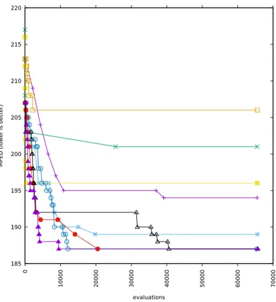
5-2 Runs with alphabets cardinality 16 and added correlation 0 . . . 62

5-3 Runs with alphabets cardinality 16 and added correlation 0.5 . . . 63

5-11 Examples ofh⇡1, ⇡2i-matching schemas for ⇡1= 3 and ⇡2 = 2 . . . 72

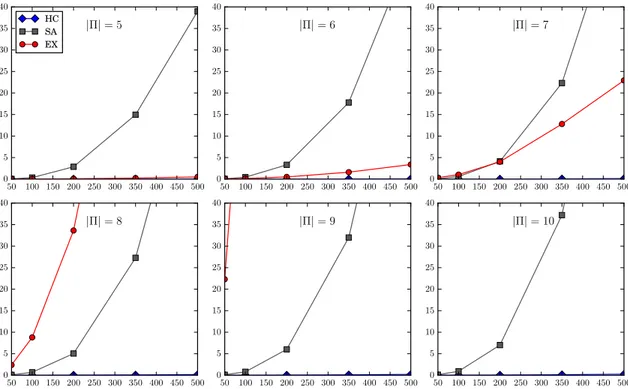
5-12 Execution time (in seconds) of HC, SA and EX against|⇧|. The four graphs, from top to bottom and from left to right, indicate the results for len(s) = 100, 200, 350 and 500, respectively. . . 79

5-13 Execution time (in seconds) of HC, SA and EX against len(s). The six graphs, from top to bottom and from left to right, indicate the result for |⇧| 2 {5..10}. . . 80

5-14 Execution time (in seconds) of HC against len(s) for several values of_{|⇧|. .} 81

5-15 Runtime comparison of ES and HC with_{|⇧| = 14, len(s) = 2000, ⇡}1= ⇡2 = 1 97

5-17 Runtime comparison of ES and HC with|⇧| = 18, len(s) = 2000, ⇡1= ⇡2 = 1 98

(16)

5-23 Comparison of mutation operators with|⇧| = 20, len(s) = 1000, ⇡1 = ⇡2 =

{1, 2, 3} . . . 105

5-24 Comparison of mutation operators with_{|⇧| = 20, len(s) = 1000, ⇡}1 = ⇡2 = {4, 5, 6} . . . 106

5-25 Comparison of mutation operators with_{|⇧| = 20, len(s) = 1000, ⇡}1 = ⇡2 = {7, 8, 9} . . . 107

5-26 Comparison of mutation operators with_{|⇧| = 20, len(s) = 1000, ⇡}1 = ⇡2 = 10 108 5-27 Comparison of ES variants with_{|⇧| = 20, len(s) = 1000, ⇡}1= ⇡2 ={1, 2, 3} 110 5-28 Comparison of ES variants with|⇧| = 20, len(s) = 1000, ⇡1= ⇡2 ={4, 5, 6} 111 5-29 Comparison of ES variants with_{|⇧| = 20, len(s) = 1000, ⇡}1= ⇡2 ={7, 8, 9} 112 5-30 Comparison of ES variants with_{|⇧| = 20, len(s) = 1000, ⇡}1= ⇡2 = 10 . . . 113

5-31 Probability distribution for a particular MPED value with|⇧| = 20, len(s) = 1000, ⇡1= ⇡2= 1 . . . 116

5-32 Probability distribution for a particular MPED value with|⇧| = 20, len(s) = 1000, ⇡1= ⇡2={2, 3, 4} . . . 117

5-33 Probability distribution for a particular MPED value with_{|⇧| = 20, len(s) =} 1000, ⇡1= ⇡2={5, 6, 7} . . . 118

5-34 Probability distribution for a particular MPED value with_{|⇧| = 20, len(s) =} 1000, ⇡1= ⇡2={8, 9, 10} . . . 119

6-1 Wireless sensor nodes deployed at DIMES. . . 125

6-2 A BMF Network. . . 126

6-3 Plot of (T)emperature and (L)ight collected from nodes a,b,c,d . . . 127

6-4 Sensitivity to sensor faults, Node (d) . . . 129

6-5 The virtual phantom used for our experimental campaign . . . 141

6-6 The clusters generated by our approach with the adoption of k-means as clustering algorithm . . . 143

6-7 The clusters generated by QuickBundles . . . 143

(17)

6-8 The 17 bundles identified in the di↵usion MR phantom adopted in our test 145

6-9 a. Approximate shape of Corpus Callosum (CC) and its axis of symmetry (black dotted line) drew by the operator; b. Extracted forcep minor of CC

fibers (green) . . . 149

6-10 a. Approximate shape of Cortico-Spinal Tract (CST) and its axis of symme-try (black dotted line) drew by the operator; b. Extracted right CST fibers (green) . . . 150

6-11 The two phantoms used in our experimental campaign . . . 153

6-12 Variation of the four performance measures against the threshold T h for each model of the phantom of Figure 6-11(a) . . . 154

6-13 Distribution of the edge weights and colored network of a control subject, a patient with MCI and a patient with AD . . . 165

6-14 Partitioning of an EEG into segments with PSWCs and without PSWCs . . 168

6-15 Colored Networks_N⇡ and N⇡ for a patient with CJD . . . 169

6-16 Connection coefficient for the network_Nblk . . . 172

6-17 Connection coefficient for the network_Nwht _{. . . .} ₁₇₂

6-18 Density for the network_Nblk . . . 173

6-19 Density for the network_Nwht _{. . . .} ₁₇₃

6-20 Clustering coefficient for the networkNblk _{. . . .} ₁₇₄

6-21 Clustering coefficient for the network_Nwht _{. . . .} ₁₇₄

6-22 The networksN0⇡ and N1⇡ for two patients with MCI at both t0 and t1 . . 176

6-23 The networks_N0⇡ and N1⇡ for two patients with MCI at t0, who converted to AD at t1 . . . 178

6-24 Results of the application of the approach of [80] to the patients of Figures 6-22 and6-23 . . . 179

(18)

(19)

List of Tables

2.1 Few examples of strings. . . 26

5.1 Parameters for Local Search heuristic . . . 55

5.2 Parameters for Simulated Annealing heuristic . . . 55

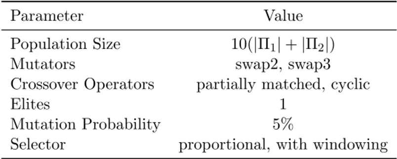
5.3 Parameters for Genetic Algorithm heuristic . . . 56

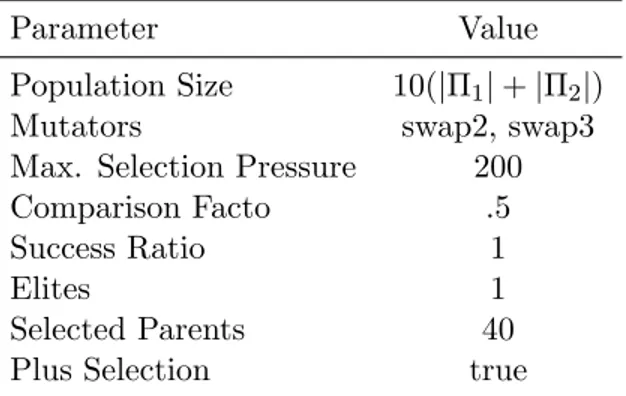
5.4 Parameters for O↵spring Selection Genetic Algorithm heuristic . . . 57

5.5 Parameters for Genetic Algorithm with ALPS heuristic . . . 57

5.6 Parameters for Evolution Strategy algorithm . . . 58

5.7 Parameters for O↵spring Selection Evolution Strategy algorithm . . . 58

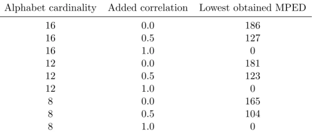
5.8 Comparative benchmark parameters for HeuristicLab heuristics comparison. 58 5.9 Lowest obtained MPED value among all runs and heuristics for HeuristicLab heuristics comparison. . . 60

5.10 HL heuristics comparison, alphabet cardinality 16 and added correlation 0 . 62 5.11 HL heuristics comparison, alphabet cardinality 16 and added correlation 0.5 63 5.12 HL heuristics comparison, alphabet cardinality 16 and added correlation 1 . 64 5.13 HL heuristics comparison, alphabet cardinality 12 and added correlation 0 . 65 5.14 HL heuristics comparison, alphabet cardinality 12 and added correlation 0.5 66 5.15 HL heuristics comparison, alphabet cardinality 12 and added correlation 1 . 67 5.16 HL heuristics comparison, alphabet cardinality 8 and added correlation 0 . 68 5.17 HL heuristics comparison, alphabet cardinality 8 and added correlation 0.5 69 5.18 HL heuristics comparison, alphabet cardinality 8 and added correlation 1 . 70 5.19 Values of PHC (left value) and PSA (right value) for di↵erent values of ⇡,|⇧| and len(s). N/A represents an instance for which the exact value cannot be computed in a feasible time. . . 78

(20)

5.21 Results for (µ + ) ES with configuration strong. . . 94

5.22 Results for (µ + ) ES with configuration medium. . . 94

5.23 Results for (µ + ) ES with configuration light. . . 95

5.24 Selected values for ES parameters. . . 96

5.25 Obtained precision of (µ + ) ES w.r.t HC. . . 102

5.26 Runtime analysis of (µ + ) ES w.r.t HC. . . 103

5.27 Selected values for ES parameters within mutation operators tests. . . 104

5.28 Estimated precision PM for each mutation operator for di↵erent values of ⇡i. 109 5.29 Estimated precision PV for each ES variant and di↵erent values of ⇡. . . 114

5.30 Configurations of (µ + ) ES for probability distribution test. . . 115

6.1 MPED and Std Correlation . . . 128

6.2 Day span . . . 128

6.3 Results for Cluster 1 . . . 142

6.7 Results obtained by applying MPEDSB and the edit distance on the 17 mod-els into consideration . . . 146

6.8 Comparison of the average Precision, Recall, F-measure and Overall obtained by applying MPEDSB and the edit distance . . . 146

6.9 Performance values obtained by our approach and QB when applied on the phantom of Figure 6-11(a) . . . 155

6.10 Performance values obtained by our approach and QB when applied on the phantom of Figure 6-11(b) . . . 155

6.11 Quantitative measures representing the colored networks of Figure6-13 . . 166

6.12 Table produced by a neurologist regarding starting and ending time-slots for each seizure of the EEG into consideration . . . 171

6.13 Quantitative measures representing the networks _N0⇡ and N1⇡ for the two patients considered in Figure6-22. . . 177

(21)

19

6.14 Quantitative measures representing the networks N0⇡ and N1⇡ for the two

patients considered in Figure6-23. . . 177

6.15 Quantitative measures representing the results shown in Figure6-24 . . . . 179

(22)

(23)

Chapter 1

Introduction

Strings play a fundamental role in computer science. Data is codified into strings by using various techniques and, by interpreting them, information can be derived. Almost every-thing in the digital world can be represented as strings: time series, access logs, astronomical data, this thesis, this exact phrase, everything that can be actually accessed. Even in the non-digital world, strings are everywhere: tram time schedules, road addresses, the plate of your car, the content of the book on your left, etc. The academic literature has been researching for many years over strings, making a fundamental theory that plays a crucial role in theoretical computer science. Information is the nourishment of computer science and with strings we encode and represent it.

From the point of view of the human society, experience strictly correlates to evolution. When we find ourselves in a novel situation, our brain automatically exploits our experience in order to understand whether we already encountered something similar to it or which is correlated to the situation itself. Terms like similarity and correlation are synonyms and represent very important concepts. These concepts also apply to computer science and to strings especially. Given a set of strings, few interesting questions arise, such as “are these strings related?”, “if they are related, how can we measure this relatedness?” and “can we define some sort of measure of (dis)similarity between strings?”. The definition of a degree of correlation or similarity between strings is strongly important: it gives us the possibility to extrapolate interesting properties, which can be used in various contexts. A straightforward example could be that of clustering a set of strings, determining whether two or more strings should be put “in the same cluster”, being sufficiently similar to each

(24)

other.

The academic community is very active on this aspect, thus di↵erent definitions of similarity/correlation between strings exist. Eventually, they steam from the concept of metric (or distance function) in mathematics, which is a function that defines a distance between each pair of elements of a set. In this case, distance is used to quantify the similarity between two strings. As an example, a famous and well-know metric in computer science is the Hamming distance, which measures the minimum number of substitutions required to change one string into the other. A large number of metrics exist and they are used in very heterogeneous contexts, such as information retrieval, machine learning, computational biology, etc.

Among these metrics, a particular one is the so called edit distance. It measures the minimum number of edit operations required to transform one string into another one. Edit operations can be of di↵erent kind, most common operations are deletions, insertions and substitutions of symbols. In this case, whether we try to define the similarity between two strings, one important natural assumption is made: identical symbols among strings represent identical information, whereas di↵erent symbols introduce, in a way or another, some form of di↵erentiation. This last assumption results to be extremely reductive. In fact, there are cases in which symbol identity seems to be not enough, and even if there are no common symbols between two strings, it could happen that they represent similar information.

Let us consider two strings generated by heterogeneous data streams, derived from two di↵erent ways of measuring the same reality; think, for instance, of two sensors one measuring light and the other measuring temperature. The values, the scales and the meaning of the two sensors may be very di↵erent, but, if sensors are near to a fire, light can be influenced by temperature, and vice versa. To properly monitor this last event, we should, then, be able to understand the correlations between these two heterogeneous measurements. In another, extreme, case, suppose one of the streams has been deliberately manipulated in such a way as to appear dissimilar from the other (think for example to code cloning techniques [67]). In this case, it can be of outmost importance being able to detect their correlation. But how can we detect the similarity between such streams?

When dealing with heterogeneous data streams, generated sequences may come from very di↵erent contexts and may be represented with di↵erent symbols/metrics.

(25)

Further-23

more, we need to take in account that providing the flexibility of mapping some symbol of the first stream into more than one symbol of the second stream (and vice versa) would be extremely useful, thus many-to-many mappings between symbols need to be considered. This is also useful, for example, to accomodate di↵erent discretization metrics of numerical sequences. Obviously, the best mapping between symbols, i.e., the one which gives the minimum distance or which discovers the optimal correlation, is not know a priori, thus searching it becomes part of the problem.

The necessity of a suitable metric capable of capturing hidden correlations between strings emerges. This metric should take into account that di↵erent symbols in the involved strings may express similar concepts. An ideal na¨ıve solution would be that of considering all of the possible correlations between symbols. However, this approach is infeasible; worse, it reduces to an intractable problem.

For a better understanding of this problem, which is discussed in detail in Chapter2, let s1= AAABCCDCAA and s2= EEFGHGGFHH be two strings. They obviously have no symbols

in common, thus resulting in being two strings completely di↵erent. However, suppose a hidden correlation exists, which matches symbols _{{A,B} with {E,H}, and symbols {C,D}} with{F,G}. Thus, the following alignment is possible:

s1 : AAABCCDDCAA! AAABCCDDCAA

s2 : EEFGHGGFHH ! -EEFGHGGFHH

** * *****

which states that the second string could be obtained from the first one with just 3 (parameterized) edit operations, thus showing a signicant, not obvious, correlation between the two strings (see Chapter4for all details). Furthermore, di↵erent mappings could exists that might give a lower number of edit operations, but enumerating them all is in fact infeasible.

There are di↵erent contexts in which such a metric can be e↵ectively used in order to approach particular problems. For instance, the engineering world is actually interested in the design, development and monitoring of wireless sensors area networks, whose com-plexity is constantly growing, thanks to the Internet of Things. Here, sensors transmit heterogeneous data, i.e., they are devices producing di↵erent kinds of signals. Challenges such as anomaly detection in this context would benefit from a metric which is capable of

(26)

discovering hidden correlations between heterogeneous series of data. And shifting away from the engineering world, the biomedical context o↵ers various scenarios in which such a metric would be useful. For example, White Matter Fiber-Bundle analysis concentrates on the investigation of brain, in which the capability of extracting, visualizing and analyzing White Matter fibers play a key role. This analysis is important because it may provide significant insights in brain functions and anomalies, in order to better understand and predict di↵erent neurodegenerative pathologies, such as multiple sclerosis. Here, providing a suitable string representation of the fibers, processes that were time consuming and error prone for a large cohort of patients would be more accessible.

In this thesis, we provide a contribution in this setting. We present a framework that generalizes most of the existing string metrics based on symbol identity making them suit-able for application scenarios where involved strings could be based on heterogeneous al-phabets. This way, our approach paves the way to the adoption of string metrics in all those contexts in which involved strings come from di↵erent sources, each adopting its own alphabet. The main components of the proposed framework are: (i) a matching schema, which formalizes matches between symbols, and (ii) a generalized metric function, which abstracts the computation of string metrics on the basis of a pre-defined matching schema. The proposed framework is based on the identification of the best matching schema for the metric function, i.e., the matching schema leading to the minimum value of the distance function when applied on the strings into consideration. We will prove the hardness of this problem, thus we provide various heuristics in order to approach it, together with a large series of tests. Then, application contexts with various contributions to each of them are presented. We highlight how the proposed framework and the specialization of it in a particular metric can be used in order to approach relevant challenges. Finally, at the end of this thesis, we draw our conclusion and we give space for future works.

The plan of the thesis is as follows: in Chapter 2 we give the background needed and we introduce fundamental concepts such as strings and distances; moreover, a review of the current related literature is provided. In Chapter 3 we introduce and define the proposed framework: few examples are given, plus we show how the framework generalizes most of the existing string metrics based on symbol identity. In Chapter 4, we formally define the Multi-Parameterized Edit Distance, a generalization of the edit distance with the support of the proposed framework, and we discuss its computational issues. Chapter 5 is devoted

(27)

25

to the presentation of the various heuristics designed and implemented in order to approach computational issues of the generalization: first, a survey on heuristics is carried out to acquire a global view of the problem, then three heuristics are selected, ad-hoc implemented and tested out. Chapter 6 is devoted to describe application contexts which have been studied in this thesis. They can be distinguished in two macro areas: engineering, with Wireless Sensors Area Networks, and biomedical informatics, with White Matter Fiber-Bundles analysis and Electroencephalogram analysis. Finally, in Chapter 7 we draw some conclusions and highlight future work.

(28)

(29)

Chapter 2

Background and Problem

Definition

2.1 Introduction

In this chapter we give an overview of the background needed for this thesis. The plan of the chapter is as follows: we first introduce fundamental concepts such as strings and similarity metrics. Then, we exploit the problems that emerge in the general context of heterogeneous alphabets and we point out the problem of discovering hidden correlations. Also, we discuss the context of our problem and its hardness. Finally, we describe an overview of the related academic literature in this context.

2.2 The fundamental concept of string

Strings essentially are ordered sequences of symbols. For a moment, we refrain to give a precise and formal definition for them. Instead, we concentrate on some examples of what a string can be, how can be represented and, most importantly, what does it mean, i.e., what is the semantic of a string. In this thesis, strings are distinguished by using a monospaced font, such as this one. Also, terms such as sequences and streams are synonyms for strings and we will often use them interchangeably in various contexts.

Table2.1 shows some examples of strings.

Strings are usually drawn from an alphabet, which is a finite and nonempty set whose elements are symbols, which are usually also called characters or letters. Thus, a string

(30)

String example abcdwxyz

0422003 010001001110 --XyX@@%115&&//

this phd thesis does not exist Table 2.1: Few examples of strings.

defined on an alphabet ⌃ is a finite sequence of elements of ⌃. The appearance of a symbol in a string is called occurrence; a symbol could occur one or more times in a string, or even zero. As an example, the alphabet the fifth string in Table 2.1 is defined on could be the set of the lowercase English letters and a space, or even simply the alphabet ⌃ =_{{d, e, h, i, n, o, p, s, t, x, } (note the space symbol).}

Alphabets can be enhanced and more structural properties can be defined. Let s = phdthsssshtdhp an example of string defined on ⌃. We denote with ⌃⇤ _{the set of all}

strings which can be defined on an alphabet ⌃. In this case, ⌃⇤ = {✏, d, dd, . . . , e, . . . }, where ✏ is the empty string, i.e., the sequence containing no symbols. Further definitions, which are defined in the next sections, will be used throughout the thesis.

2.3 Similarity, correlation and distance

Given a pair of strings, some interesting questions arise, such as “are these strings related?”, “if they are related, how can we measure this relatedness?” and “can we define some sort of measure of (dis)similarity between strings?”. In particular, such questions give us as results the possibility to extrapolate interesting properties, which could be used in various contexts. As an example, suppose we would need to cluster a set of strings S. A cluster S 2 S in this case would be represented by all of the strings s 2 S which are “close” or “similar” to each other. Thus, a definition of similarity is needed.

The good news is that such a defintion, which strictly depends on the approach used to compute it, already exists. The first (and also most famous) approach is that of the Hamming distance [55], introduced by Richard Hamming as a geometrical model for error detecting codes. Into the space of _{{0, 1}}n _{points, Hamming introduced a distance, better}

know by its mathematical term metric, D(x, y), where x, y 2 {0, 1}n_{. The definition of}

(31)

2.3. SIMILARITY, CORRELATION AND DISTANCE 29

coordinate, two errors, two coordinates, etc. Thus, the distance D(x, y) between two points x and y is defined as the number of coordinates for which x and y are di↵erent. D(x, y) is a metric, as shown in [55].

Let s1 = 0100110 and s2 = 0110100 be two strings. Clearly, D(s1, s2) = 2 and we

visualize this results by drawing s1 and s2 one below the other. Additionally, in the row

below the last string we denote with the symbol * a position in which s1 and s2match, e.g.,

they have a symbol in common.

s1: 0100110

s2: 0110100

** ** *

It is straightforward to see that the Hamming distance can be applied only on points defined on the same space, e.g., the number of components of points has to be the same.

What about points defined on di↵erent spaces? More general, can Hamming distance be defined on generic strings? It seems the answer is no, thus a di↵erent metric is needed to work with.

Back to 1965, Vladimir Iosifovich Levenshtein, working on information theory and error-correcting codes, introduced a metric for codes capable of error-correcting deletions, insertions and reversal [75]. This was later called Levenshtein distance and is informally defined as the minimum number of single-symbol edits, i.e., edit operations, which are deletions, insertions and substitutions, required to change one string into the other, where each operation has a cost assigned to. As for an example, let s1 = ATGCA and s2 = GGCA two strings and let

D(x, y) the Levenshtein distance between x and y. Suppose that deletions, insertions and substitution respectively have cost equals to 1, 1 and 2. D(s1, s2) is 3 and we can (possibly)

obtain it by

1. inserting symbol A at beginning of s2 (cost 1),

2. substituting symbol G (first one) with symbol T in s2 (cost 2).

It is straightforward to see that numerically D(s1, s2) depends on the cost assigned to each

edit operation. Moreover, there could be di↵erent ways of applying edit operations in order to obtain D(s1, s2).

(32)

definition of an edit distance use di↵erent sets of symbol or string operations. Other exam-ples of edit distances are the longest common subsequence (LCS) which allows deletions and insertions but substitutions, or the Jaro distance [65] which allows only transposition. Also, Hamming distance is an edit distance, allowing only substitutions, thus it can be applied only on strings of the same length. Edit distance essentially represents a parametric metric, equipped with a set of allowed edit operations and to each operation a cost is assigned.

In [113], Wagner and Fischer proposed an algorithm for determining a sequence of edit transformations that changes one string into another, i.e., computing the edit distance, using the same three edit operations used in the Levenshtein distance with cost being parameterized. Their algorithm is proportional to the product of the lengths of the two input strings and it represents one of the earliest problem of dynamic programming studied by all of computer science students.

During this thesis, when it is not di↵erently specified, we will use (classical) edit distance and Levenshtein distance as synonyms, and we will make use of the algorithm presented in [113] for the implementation. Moreover, we will use the term alignment in the classical term, representing a number of edit operations needed to transform a string into another.

2.4 The real problem

As pointed out in the previous sections, various string metrics exist and they may signifi-cantly di↵er for the rules adopted to measure the (dis)similarity degree; it appears obvious that these rules depend on the context in which they are applied. For example, in [43] a survey on duplicate record detection in databases indicates di↵erent string metrics with di↵erent allowed edit operations which have been specifically tailored for the application context. However, it is important to point out that most of available metrics are based on the natural assumption that identical symbols among strings represent identical information, whereas di↵erent symbols introduce, in a way or another, some form of di↵erentiation.

Let s = AAABCD and t = 111234: any standard metric would state that they are completely di↵erent. Nevertheless, there are cases (like the one shown above) in which symbol identity seems to be not enough. In fact, even if there are no common symbols between two strings, it could happen that they somehow represent similar information.

(33)

2.5. RELATED WORK 31

two strings that apparently have di↵erent symbols but similar structures? As an example, consider two strings s and t and assume that they are generated by heterogeneous data streams, derived from two di↵erent ways of measuring the same reality; think, for instance, of two sensors one measuring light and the other measuring temperature. The values, the scales and the meaning of the two sensors may be very di↵erent, but, if sensors are near to a fire, light can be influenced by temperature, and vice versa. To properly monitor this last event, we should, then, be able to understand the correlations between these two heterogeneous measurements. As a further example, suppose that s and t have been deliberately manipulated in such a way as to appear dissimilar, even if their meaning is actually identical - think, for instance, of code cloning techniques [67]. In these cases, the necessity arises of a suitable metric capable of capturing hidden correlations between strings. This metric should take in account that di↵erent symbols in the involved strings may express similar concepts.

2.5 Related work

String similarity computation has been a challenging issue in the past literature, and several attempts to face this problem have been presented. However, most of the literature gener-alizing classical approaches with parameterized alphabets focuses on the pattern matching problem (starting from [10]), where the objective is to seek (exact or approximate) occur-rences of a given pattern in a text. This is the context in which parameterized strings were introduced. Here, some of the symbols act as parameters that can be properly substituted at no cost; in approximate pattern matching, patterns have a parameterized match with a text if at most k mismatches occur [77].

A seminal work on this topic is presented in [10]. The approach described in this paper compares parameterized strings. It considers bijective global transformation functions allowing exact p-matches only. This means that the two strings to match must have the same length; thus, no substitutions or insertions are allowed.

Mismatches are allowed in [57], where the authors face the problem of finding all the locations in a string s for which there exists a global bijection ⇡ that maps a pattern p into the appropriate substring of s minimizing the Hamming distance. From the function viewpoint, injective functions, instead of bijective ones, are considered in [6].

(34)

String matching has been extensively used for the clone detection problem, i.e., to check if a code contains two or more cloned parts. In [67], a token-based code clone detection approach is presented. Here, matches between strings are carried out by using a suffix-tree algorithm. The code is tokenized by only one parameter; thus, a match is represented by a one-to-many mapping.

The work in [5] introduces the concept of generalized function matching applied to the pattern matching problem in several contexts, like image searching, DNA analysis, poetry and music analysis, etc.

The authors in [44] carry out a comprehensive complexity analysis of the pattern match-ing problem with parameters (called variables in this paper) with several configurations (e.g., exploiting injective or non-injective functions, allowing or disallowing deletions, etc.). They show that most of the considered variants are NP-complete problems. A detailed survey on parameterized matching appears in [83].

Moving towards string similarity computation, a relevant research issue regards the longest common subsequence problem (hereafter, LCS) and its parameterized versions. Some interesting approaches to facing this problem can be found in [16], [92], and [69]. Specifically, in [16], the definition of arc-annotated sequences is used, [92] considers the gapped version of LCS, whereas in [69] the parameterized version of the LCS problem is considered. Interestingly, LCS allows only insertions and deletions, but no substitutions.

String similarity metrics present important overlap with approximate pattern match-ing, since one can determine the distance between two strings asking whether there exists an approximate pattern matching with at most k mismatches. However, having a direct approach for measuring the parameterized distance provides obvious benefits.

Few works consider the problem of parameterized distances between strings. In [11], the notion of p-edit distance is introduced. It focuses on the edit distance, where allowed edit operations are insertions, deletions and exact p-matches. Mismatches are not allowed. Fur-thermore, two substrings that participate in two distinct exact p-matches are independent of each other, so that mappings have local validity over substrings not broken by insertions and deletions. In particular, within each of these substrings, the associated mapping func-tion must be bijective. The work presented in [69] extends the approach proposed in [11] by requiring the transformation function to have a global validity; however, it still limits the set of allowed edit operations (in particular, substitutions are not possible).

(35)

2.5. RELATED WORK 33

The work in [50] is based on the approach proposed in [10]; it introduces an order-preserving match, but it limits the number of mismatches to k. In [54], a preliminary approach to a many-to-many mapping function for string alignment can be found; it com-putes alignments between two parameterized strings and gives preferences to alignments on the basis of the co-occurrence frequency.

Moreover, it is worth to recall that edit distance has been exploited in the problem of sequence alignment in the bioinformatics context. Here, two symbolic representations of DNA or protein sequences are aligned in order to identify regions of similarity. The comparison aims at looking for evidence that two sequences have diverged from a common ancestor by a process of mutation and selection [39]. Classical edit operations here are intended as the basic mutational processes that are insertions and deletions (also called gaps), which add or remove residues, and substitutions, which change residues in a sequence. Alignments in pairwise alignment are scored by the sum of terms for each aligned pair of residues and each aligned residue pair is scored by using a scoring matrix. Scoring matrices, also called substitution matrices, are matrices which store the score assigned to a pair of aligned residues. Two main categories of scoring matrices exist in literature, namely (i) position-independent and (ii) position-specific scoring matrices. The former category includes well-known scoring matrices such as PAM and BLOSUM [60,100], while the latter includes scoring matrices used in protein BLAST [4]. Scoring matrices in both categories are defined upon specific alphabets, e.g., nucleotides or amino acids, and over homogeneous sequences, thus the heterogeneous case is not applicable.

(36)

(37)

Chapter 3

Generalizing identity-based string

comparison metrics

3.1 Introduction

In this chapter, we formally introduce the theoretical foundation of our work. In particular, we define and analyze the framework F, which is intended to generalizing identity-based string similarity metrics. We first give the formal basis by defining important preliminary concepts and then we introduce matching schemas and generalized metric functions, which are the main ingredients for the framework F. Finally, we show how the introduced frame-work can be exploited to generalize some notable string similarity metrics. Each section is correlated by various examples.

Part of the work proposed in this chapter has been published in [30].

3.2 Preliminaries

In a general context, let ⇧1 and ⇧2 be two (possibly disjoint) alphabets of symbols and let

s1 and s2 be two strings defined over ⇧1 and ⇧2, respectively. We denoted the length of a

string s, i.e., the number of its symbols, by len(s1). We refer to a symbol in s by accessing

its position: for each position 1 _{ j  len(s), the j-th symbol of s will be identified by} si[j] and we will denote the substring of s starting at position x and ending at position y

as s[x..y].

(38)

to use a special concept called matching schema which intuitively represents how di↵erent combinations of the alphabets ⇧1 and ⇧2 can be combined via matching. A matching

schema is extremely important for the definition of F.

Definition 1 (⇡-partition) Given an alphabet ⇧ and an integer ⇡ such that 0 < ⇡ |⇧|, a ⇡-partition is a partition ⇡ _{of ⇧ such that 0 <}_|

v|  ⇡, for each v 2 ⇡. ⇤

Definition 2 (_h⇡1, ⇡2i-matching schema) Given two alphabets ⇧1 and ⇧2 and two

inte-gers ⇡1and ⇡2, ah⇡1, ⇡2i-matching schema is a function M_h⇡1,⇡2i:

⇡1

1 ⇥ ⇡22 ! {true, false},

where ⇡i

i (i2 {1, 2}) is a ⇡i-partition of ⇧i and, for each v 2 1⇡1 (resp., w 2 ⇡22), there

is at most one w 2 ⇡22 (resp., v 2 ⇡11) such that M ( v, w) = true. This means that

all the symbols in v match with all the ones in w. M ( v, w) = false indicates that all

the symbols in v mismatch with all the ones in w. ⇤

Intuitively, a ⇡-partition ⇡ is a subset of _{P(⇧) where each subset} v 2 ⇡ contains

at most ⇡ symbols from ⇧ and for each v, w 2 ⇡, v \ w = ;, i.e., they contain

no common symbols. Using two ⇡-partitions, given two strings s1 and s2 defined over

two alphabets ⇧1 and ⇧2, a h⇡1, ⇡2i-matching schema states which symbols of s1 can be

considered matching with symbols of s2. It is essential to note that many-to-many matching

are actually expressed with ⇡-partitions and at the same time they disallow ambiguous matchings.

Example 1 Let ⇧1 = {A, B, C, D} and ⇧2 = {E, F, G, H}. Let s1 = AAABCCDCAA and

s2 = EEFGHGGFHH. The values of ⇡1 and ⇡2 define the cardinality of each subset in a

⇡-partition. For ⇡1= ⇡2 = 2, one (of the many) possible matching schemas is{{A,B}-{E,H},

{C,D}-{G,F}}. Note that here {A,B}-{E,H} means that symbols A and B match with symbols E and H. As a further example, having ⇡1 = ⇡2 = 1, a possibile matching schema

is{{A}-{E}, {B}-{G}, {C}-{F}, {D}-{H}}.

It is interesting to point out that, given ⇧1, ⇧2, ⇡1 and ⇡2, many possible matching

schemas can be defined. However, in some contexts, it may be useful to limit valid matching schemas via some constraints (a real example is given in Section6.3). In order to provide this possibility, the following definition formally introduces both the notions of constraint(s) over a matching schema and constrained matching schema.

(39)

3.2. PRELIMINARIES 37

Definition 3 (h⇡1, ⇡2, i-constrained matching schema) A constraint associated with

a matching schema M_h⇡₁_,⇡₂_iis a set of unordered pairs of symbols (ci, cj), such that ci 2 ⇧1,

cj 2 ⇧2 and, for each (ci, cj)2 , there exists no pair ( v, w), v 2 1⇡1, w 2 2⇡2,

hav-ing ci 2 1, cj 2 2 and M ( 1, 2) = true. A h⇡1, ⇡2, i-constrained matching schema is

represented by M_h⇡₁,⇡2, i only if 6= ;. ⇤

Example 2 Continuing the Example1, suppose we have =_{{(B, H), (C, F)}, the matching} schema represented by {{A,B}-{E,H}, {C,D}-{G,F}} is no more valid, whereas the matching schema represented by _{{{A,B}-{E,F}, {C,D}-{G,H}} is.}

Throughout the whole thesis, whenever it is clear from the context, for the sake of simplicity, we avoid to write M_h⇡₁_,⇡₂_, _i and we simply denote it by M .

The generalizability of the framework F is based on the fact that it can generalize any string metric based on the assumption of symbol identity. Therefore, in defining it, we are not interested in a particular function specification, rather in a generalization of a metric function.

Definition 4 (Generalized metric function) Given a metric function f (·, ·), based on symbol identity, and given a valid constrained matching schema M , the generalized metric function fMh⇡1,⇡2, i₍_{·, ·) (or simply f}M₍_{·, ·)) is obtained from f(·, ·) by substituting symbol}

identity with the symbol matchings defined in M . ⇤

Having a generalized metric function, we now need to formally define the result of the application of it, i.e., the distance given by the application of the metric. In this case, the obtained distance depends on M and f .

Definition 5 (Generalized distance) Given two strings s1 and s2 over ⇧1 and ⇧2,

re-spectively, and given the set M of valid constrained matching schemas, the generalized distance F (s1, s2) between s1 and s2 returns the minimum value returned by fM(s1, s2)

that can be obtained by taking any possible matching schema M of M. Formally:

F (s1, s2) = min M_{h⇡1,⇡2, i}2M{f

M_(s

1, s2)}.

(40)

Finally, we defined all of the bricks needed in order to build the framework F. In Section3.3 we formally define the framework and we give the intuition behind it.

3.3 The framework

Thanks to the definitions in Section 3.2, we are now able to present our framework F. It consists of a quintuple:

F =_h⇧1, ⇧2,h⇡1, ⇡2, i, M, fM(·, ·)i

where ⇧1 and ⇧2 are the alphabets on which the strings under consideration are defined,

h⇡1, ⇡2, i are the parameters necessary to define valid matching schemas, M is the set of

all the valid constrained matching schemas over ⇧1 and ⇧2, and fM(·, ·) is the generalized

metric function. When applied on two strings s1 and s2 over the alphabets ⇧1 and ⇧2,

respectively, F returns the value of F (s1, s2), where F (s1, s2) is the generalized distance of

s1 and s2 over f (·, ·) and M.

3.4 Generalization of notable string similarity metrics

In the previous sections, we introduced our framework F, which paves the way to a quite general computation of string (dis)similarity. We are now ready to show that F is general enough to encompass several classical and notable string similarity metrics. Our idea is to first show that a particular specialization of F includes both character-based and token-based distances; starting from this, we show that F can also be specialized to more sophisticated comparison approaches, such as parameterized pattern matching proposed in [10].

Proposition 1 Given the following specialization of F:

1. ⇡1 = ⇡2 = 1;

2. =_{(ci, cj)|ci2 ⇧1, cj 2 ⇧2, ci6= cj};

then, fM(_{·, ·) = f(·, ·) for all the metric functions f(·, ·) based on symbol identity.} ⇤ The reason behind the Proposition1is that, intuitively, with ⇡1 = ⇡2= 1, the cardinality

(41)

3.4. GENERALIZATION OF NOTABLE STRING SIMILARITY METRICS 39

Furthermore, with the provided construction of , only symbol identities are allowed. As a consequence, there is only one valid matching schema M_{h1,1, i}, which is the one stating that, for each pair ( v, w), v 2 ⇡₁1 and w 2 ⇡₂2, M ( v, w) = true if and only if v = w.

This matching schemas simulates symbol identity specification for the generalized metric functions based on symbol identities.

In the following subsections, we show how our framework F, according to Proposition1, can be used to generalize some notable string similarity metrics.

3.4.1 Edit Distance

In its simplest form, the edit distance between two strings s1 and s2 is the minimum

number of edit operations (insertions, deletions or substitutions) of single characters needed to transform s1 into s2, where each operation has a cost equal to 1 [75]. This version of

the edit distance is also referred to as Levenshtein distance. A basic algorithm for edit distance computation exploits a dynamic programming approach; in it, the choice of the edit operation is carried by a recurrence formula, where the discriminating factor is based on the question “Is s1[i] = s2[j]?”.

If our framework F is applied, this question is substituted by the question “According to M , symbols s1[i] and s2[j] should be matched?”. As specified by Proposition1, according to

the specialization defined therein, this question is equivalent to asking for symbol identity.

3.4.2 Affine Gap Distance

The affine gap distance metric [116] is similar to the edit distance, except for the fact that it introduces two extra edit operations, i.e., open gap and extend gap. In this way, the cost of the first insertion (gap opening) can be di↵erent from, and is usually higher than, the cost of adding consecutive insertions (gap extensions). Similarly to the edit distance, the discriminating factor in computing the affine gap distance is based on the question “Is s1[i] = s2[j]?”. When applying our framework F with the specialization introduced in

Proposition1, this question is substituted by the one “According to M , symbols s1[i] and

s2[j] should be matched?”, which has been shown to be equivalent to asking for symbol

(42)

3.4.3 Smith-Waterman Distance

The Smith-Waterman distance [104] is an extension of both the edit distance and the affine gap distance, in which mismatches at the beginning and the end of strings have lower costs than mismatches in the middle. This metrics allows for substring matchings and is well suited for fitting shorter strings into longer ones. Also in this case, the basic resolution schema exploits dynamic programming, where the discriminating factor in the recurrence formula is the question “Is s1[i] = s2[j]?”.

3.4.4 Jaro Distance Metric

The Jaro distance metric, introduced in [65], is based on the concepts of common characters and transpositions.

Given two strings s1 and s2, two symbols s1[i] and s2[j] are common characters when

s1[i] = s2[j] and|i j|  1₂min{len(s1), len(s2)}. Given the i-th common character a in s1

and the j-th common character b in s2, if a6= b this is a transposition.

The Jaro distance value is, then, computed as:

Jaro(s1, s2) = 1 3 c len(s1) + c len(s2) +c 1 2t c !

where c is the number of common characters and t is the number of transpositions.

The characteristics of the Jaro distance metric clearly di↵er from the ones of the afore-mentioned metrics. However, as a common core for the definitions of common character and transposition, there is, again, symbol equality, where the discriminating question is “Is s1[i] = s2[j]?”.

Also in this case, it is easy to show that substituting this question with the one “Ac-cording to M , symbols s1[i] and s2[j] should be matched?”, under the specialization of

Proposition1, makes the two settings equivalent.

3.4.5 Atomic Strings

In atomic strings [86], the comparison shifts away from single character to longer strings. In particular, s1 and s2 are tokenized by punctuation characters. Each token is called atomic

(43)

3.4. GENERALIZATION OF NOTABLE STRING SIMILARITY METRICS 41

similarity between s1 and s2 is, then, computed as the fraction of the atomic strings that

match.

Observe that, even if this metrics moves from the comparison of single characters to the one of substrings, the basic operation used to identify a matching for atomic strings is the identity of sequences of single characters. As a consequence, the same considerations outlined above when substituting the question “Is s1[i] = s2[j]?” with the one “According

to M , symbols s1[i] and s2[j] should be matched?” are still valid.

3.4.6 WHIRL

In [33] the cosine similarity is combined with the tf.idf weighting scheme in the WHIRL system to compare pairs of strings in a set of records. In particular, each string s is separated into words; a weight vs(w) is assigned to each word w of s, which depends on the number

tfw of times when w appears in s and on the fraction idfw of records containing w. The

cosine similarity between two strings s1 and s2 is, then, defined as:

sim(s1, s2) =

⌃wvs1(w)· vs2(w)

||vs1||2· ||vs2||2

.

Despite the complexity of this metric, as for its application to our context, the most relevant thing to observe is that both the tfw and the idfw components are based on the exact

occurrence of w in the string(s). As a consequence, again, when asking whether a word w is contained into a string s, the basic question for the computation is “Is w[i] = s[j]?”, which, as previously shown, can be simulated by the question “According to M , symbols w[i] and s[j] should be matched?”, under the specialization of Proposition1.

3.4.7 Q-grams with tf.idf

Q-grams with tf.idf [53] extends the metric adopted in WHIRL by using q-grams, instead of words. This allows the management of spelling errors, the insertion and the deletion of words. The computation setting is equal to the one of WHIRL; therefore, all considerations about the specialization of F seen for WHIRL can be applied also to this metrics.

(44)

3.4.8 Parameterized pattern matching

In [10], an approach to comparing strings over partially overlapping alphabets is proposed. This approach, named parameterized pattern matching, aims at identifying pairs of strings being equal except for a one-to-one symbol substitution. In particular, the alphabet of each string si is partitioned in two alphabets, namely ⌃i and ⇧i, the former containing standard

symbols and the latter encompassing parameters. Parameters can be renamed at no cost. Two such strings identify a parameterized match if one string can be obtained by renaming the parameters of the other by means of a one-to-one function. This approach has been shown to be particularly useful in code cloning identification.

Our framework can be specialized to accommodate parameterized pattern matching. In fact, given two strings s1and s2, defined over the alphabets ⌃1[⇧1and ⌃2[⇧2, respectively,

consider the following specialization of F:

1. ⇡1 = ⇡2 = 1;

2. =_{(ci, cj)|ci2 ⌃1, cj 2 ⌃2, ci6= cj};

Let f (_{·, ·) be the Hamming distance (which, basically, is the edit distance allowing} symbol substitutions only). If F (s1, s2) = 0, then there is a parameterized matching between

s1 and s2.

In particular, ⇡1 = ⇡2= 1 constraints to one-to-one functions. The definition of states

that the only valid match configuration between pairs of symbols in ⌃1 and ⌃2 is symbol

identity, whereas any symbol in ⇧1 (resp., in ⇧2) can be matched at no cost, by means

of a one-to-one matching function, with any symbol of the other string. F (_{·, ·) finds the} minimum value of the Hamming distance, among all the possible one-to-one substitutions. A value of this distance equal to 0 denotes that one string can be obtained by renaming the parameters of the other by means of a one-to-one function and, consequently, that a parameterized match holds.

(45)

Chapter 4

Multi-Parameterized Edit Distance

4.1 Introduction

In this chapter we formally define one of the most important result derived from the frame-work F, showing how it can be applied to generalize a classic metric in such a way that symbol identity is substituted by many-to-many symbol correlations, with respect to the general idea and motivation behind it given in Chapter1, where identifying the best match-ing schema is part of the problem. Furthermore, this chapter focuses on studymatch-ing in detail all of the theoretical and practical implications of this generalization. We introduce the Multi-Parameterized Edit Distance (MPED), which is a generalization of the classical edit distance with the support of our framework. The MPED allows the computation of the minimum edit distance between two strings, provided that finding the optimal matching schema, under a set of constraints, is part of the problem. This chapter is organized as fol-lows: in Section4.2we introduce some basic definitions and the definition of MPED. Then, in Section 4.3 some examples are presented in order to give to the reader some insights on the problem in instance. Finally, in Section 4.4 computational issues are discussed. In particular, the NP-Hardness of the problem and a lower bound L are analyzed in depth.

Part of the work presented in this chapter is included in [30].

4.2 Definitions

Definition 6 (Transposition) Let s1 and s2 be two strings defined over the alphabets

(46)

(i2 1, 2) is a transposition of si if ¯si can be obtained from si by deleting all the occurrences

of . The set of all the possible transpositions of si is denoted byT R(si). ⇤

Definition 7 (Alignment) An alignment for the strings s1 and s2 is a pairh¯s1, ¯s2i, where

¯

s1 2 T R(s1), ¯s2 2 T R(s2) and len(¯s1) = len(¯s2). Here, is meant to denote an

inser-tion/deletion operation performed on s1 or s2. ⇤

Definition 8 (Match and distance) Let_h¯s1, ¯s2i be an alignment for s1and s2, let M_h⇡1,⇡2, i

be ah⇡1, ⇡2, i-constrained matching schema over ⇡-partitions ⇡11 and ⇡22 and the set of

constraints , and let j be a position with 1_{ j  len(¯s}1) = len(¯s2). We say thath¯s1, ¯s2i

has a match at j if:

• s1[j]2 v, s2[j]2 w, v 2 ⇡₁1, w 2 ⇡₂2 and M_h⇡1,⇡2, i( v, w) = true.

The distance between ¯s1 and ¯s2 under M_h⇡1,⇡2, i is the number of positions at which the

pair h¯s1, ¯s2i does not have a match. ⇤

Given the previous definitions, we can introduce the notion of Multi-Parameterized Edit Distance between two strings s1 and s2 as follows:

Definition 9 (Multi-Parameterized Edit Distance - MPED) Let ⇡1 and ⇡2 be two

integers such that 0 < ⇡1 |⇧2| and 0 < ⇡2  |⇧1|; the Multi-Parameterized Edit Distance

between s1and s2(Lh⇡1,⇡2, i(s1, s2), for short) is the minimum distance that can be obtained

with any_h⇡1, ⇡2, i-constrained matching schema and any alignment h¯s1, ¯s2i.

Formally: F_L=h⇧1, ⇧2,h⇡1, ⇡2, i, M, LM(·, ·)i and F_L(s1, s2) =L_h⇡1,⇡2, i(s1, s2) = min M_{h⇡1,⇡2, i}2M{L M_(s 1, s2)}.

where_{L(·, ·) is the classical edit distance.} ⇤

Observe that, in order to properly compute Lh⇡1,⇡2, i(s1, s2), several components play a

(47)

4.3. EXAMPLES 45

• ⇡1 and ⇡2, which determine the (maximum) size of each partition;

• ⇡-partitions ⇡1

1 and ⇡22; in fact, there can be many ⇡-partitions for the same set of

⇡1, ⇡2, ⇧1, and ⇧2;

• matching schemas Mh⇡1,⇡2, i, which determine the way to combine partitions of

dif-ferent sets via matching;

• alignments; in fact, there can be many possible alignments between two strings. Moreover, note how plays a crucial role in the computation of MPED. In fact, when is not empty, it means that additional information about which symbols should not match is injected in the computation. In order to reinforce this concept and to point out that some a priori knowledge might be available, even if not complete, we enrich the notion of MPED with a particularly common case, i.e., when identical symbols should be considered as matching anyway, yet allowing many-to-many matching in the matching schema. We call this specific case Semi Blind Multi-Parameterized Edit Distance and we formally define it enriching Definition8 as follows:

Definition 10 (Semi-Blind Multi-Parameterized Edit Distance - MPEDSB) The

Semi-Blind Multi-Parameterized Edit Distance (MPEDSB for short) is obtained from MPED by

considering a match between _hs1, s2i at j if (cfr Definition 8):

• s1[j]2 v, s2[j]2 w, v 2 ⇡11, w 2 ⇡22 and Mh⇡1,⇡2, i( v, w) = true,

• s1[j] = s2[j].

Observe that this concept might be further generalized with matchings that should always hold (as opposit to constraints, specifying matchings that must not hold). However, this is a less interesting case, in practice.

4.3 Examples

Example 3 Let s1 = AAABCCDCAA and s2 = EEFGHGGFHH, which determines ⇧1 =

{A,B,C,D} and ⇧2 ={E,F,G,H}. For ⇡1 = ⇡2 = 1, the best alignment h¯s1, ¯s2i that can

be computed is obtained by matching {A}-{E}, {B}-{G}, {C}-{H}, and {D}-{F}. The aligment:

(48)

s2 : EEFGHGGFHH ! EEFGHGGFH-H

** ** **

gives_L_h1,1i(s1, s2) = 5. Observe that this approach works properly even if ⇧1\ ⇧2 =; and

the input strings have di↵erent lengths.

If we set ⇡1 = ⇡2 = 2, the best alignment is the one obtained by matching{B,A}-{E,H},

and _{{C,D}-{G,F}, namely:}

s2 : EEFGHGGFHH ! -EEFGHGGFHH

** * ***** which gives _L_h2,2i(s1, s2) = 3.

Suppose, now, to introduce the constraint = _{{hA, Ei}. For ⇡}1 = ⇡2 = 1, the best

alignment _h¯s1, ¯s2i is the following:

s1 : AAABCCDDCAA! AAABC-CDDCAA

s2 : EEFGHGGFHH ! --EEFGHGGFHH

** *****

which still gives _L_{h1,1, i}(s1, s2) = 5, but where A and E do not match anymore. Optimal

matchings are, in fact, {A}-{H}, {B}-{E}, {C}-{F}, and {D}-{G}. ⇤

4.4 Computational issues: complexity

4.4.1 NP-Hardness

After having defined MPED, it is important to analyze its properties. We start by de-termining its computational complexity. The specialization of F provided in Proposition 1

ensures that, in that case, there exists only one valid matching schema inM, and this can be easily derived by construction. However, in general,M could contain n matching schemas; each matching schema M_h⇡₁,⇡2, i 2 M could match ⇡1 symbols of ⇧1 with ⇡2 symbols of ⇧2;

furthermore, for each matching schema, several alignments between s1 and s2 are possible.

(49)

4.4. COMPUTATIONAL ISSUES: COMPLEXITY 47

Theorem 1 The problem of computingLh⇡1,⇡2, i(s1, s2) is NP-Hard.

Proof.

This theorem can be proven by performing a reduction from the three-dimensional matching problem (hereafter, 3DM) [48]. First recall that 3DM is defined as follows:

Let X, Y and Z be finite and disjoint sets, and let M be a subset of X⇥ Y ⇥ Z. That is, M consists of triples hXi, Yi, Zii such that Xi 2 X, Yi 2 Y , and Zi 2 Z.

Now, M0 _{✓ M is a 3DM if, for any two distinct triples hX}₁_{, Y}₁_{, Z}₁_{i 2 M}0 _and

hX2, Y2, Z2i 2 M0, we have X1 6= X2, Y1 6= Y2, and Z1 6= Z2.

The decision problem is, then, stated as follows: given a set M and an integer k, decide whether there exists a 3DM M0 ✓ M such that |M0_| _k.

Let us, now, turn to the reduction. Let Mi indicate the i-th triple in M and let q =|M|.

Let ⇧1 = X [ Y [ Z [ ⌃ and ⇧2 = {Mi} [ ⌃, where the pairs (Xi, Mj) (resp., (Yi, Mj),

(Zi, Mj)) are not constrained, i.e., any of these pairs can possibly match.

For each triple Mi, ⌃ contains the set of symbols {ci1. . . ciq, ti1. . . ti7, mi1. . . mi7}; the

set of constraints is constructed in such a way as to allow symbol identity only among the symbols in _{ci1. . . ciq, ti1. . . ti7, mi1. . . mi7}.

Then, starting from M , we build the following strings:

s1 = 1 c11 c12 · · · c1q 2 c21 c22 · · · c2q · · · q cq1 cq2 · · · cqq

s2 = 1 c11 c12 · · · c1q 2 c21 c22 · · · c2q · · · q cq1 cq2 · · · cqq

where, for each triple Mi, the “blocks” i and i have the form:

ti1 Xi ti2 ti3 ti4 Yi ti5 ti6 ti7 Zi

Mi mi1 mi2 Mi mi3 mi4 mi5 Mi mi6 mi7

To clarify this construction, consider the set M = {hX1, Y2, Z2i, hX2, Y1, Z1i, hX3, Y2, Z3i,

Generalizing identity-based string similarity metrics: theory and applications

Universit`

a della Calabria

Dipartimento di Matematica e Informatica

Dottorato di Ricerca in Matematica e Informatica

XXX ciclo

Generalizing Identity-Based String

Similarity Metrics:

Theory and Applications

Settore Disciplinare INF/01 – INFORMATICA

Coordinatore: Ch.mo Prof. Nicola Leone

Supervisore:

Prof. Giorgio Terracina

Acknowledgments

Abstract

Sommario

Contents

List of Figures

List of Tables

Chapter 1

Introduction

Chapter 2

Background and Problem

Definition

2.1

Introduction

2.2

The fundamental concept of string

2.3

Similarity, correlation and distance

2.4

The real problem

2.5

Related work

Chapter 3

Generalizing identity-based string

comparison metrics

3.1

Introduction

3.2

Preliminaries

3.3

The framework

3.4

Generalization of notable string similarity metrics

Chapter 4

Multi-Parameterized Edit Distance

4.1

Introduction

4.2

Definitions

4.3

Examples

4.4

Computational issues: complexity