Published by Canadian Center of Science and Education
Convolution Based Unit Root Processes: a Simulation Approach
Fabio Gobbi1 1Department of Statistics, University of Bologna
Correspondence: Fabio Gobbi, Department of Statistics, University of Bologna. E-mail: [email protected] Received: August 4, 2016 Accepted: August 22, 2016 Online Published: October 17, 2016
doi:10.5539/ijsp.v5n6p22 URL: http://dx.doi.org/10.5539/ijsp.v5n6p22 Abstract
We propose a convolution based approach to the simulation of a modified version of a unit root process where the state variable Yt−1is dependent on the innovationεt. The dependence structure is given by a copula function C. We study by
simulation the effect of a negative correlation on the properties of unit roots. We call this process C-UR(1). Keywords:unit root processes, C-convolution, stationarity.
1. Introduction
In this paper we present a modified version of a unit root processes using a convolution-based technique. This method-ology exploits the properties of copula functions. The application of copula functions to stochastic processes (more in particular to Markov processes) was recently described in the book by Cherubini, Gobbi, Mulinacci and Romagnoli (2012). Our contribution relies on the application of a particular family of copulas, which are generated by the convo-lution operator, to the design of time series processes. From this point of view, the paper contributes to the literature modeling time series with copulas (Chen & Fan, 2006; Chen, Wu, & Yi, 2009; Cherubini & Gobbi, 2013). While this literature builds on the pioneering paper by Darsow, Nguyen and Olsen (DNO, 1992) on the link between copula functions and Markov processes, our paper exploits the concept of convolution based copulas to define a new version of the unit root process. Beyond the Markov property, there is a long standing and extremely vast literature on the fact that most of the changes of the processes, those that are called innovations, are not predictable on the basis of past information (Samuelson, 1963; 1973; Fama, 1965). In financial markets the natural representation of this concept is to assess that log-prices of assets follow a random walk, which is, in fact, a unit root process. Technically, this process is character-ized by innovations that are permanent and independent of the level of the process. The same random walk hypothesis spread into the literature in the field macroeconomics in the 1980s, starting with the seminal paper by Nelson and Plosser (1982). Based on the first unit root tests, due to Dickey-Fuller (1979; 1981), Nelson and Plosser found that most of the US macroeconomic time series included a random walk component, that is a shock, independent and persistent. In this paper we propose an extension to this approach, which allows for dependent innovations, and for non linear dependence between the innovation and the value of the process of the previous period. This is our modified version of the unit root process. The dependence structure is modelled by a copula function and the distribution of the process for all t is obtained by applying the C-convolution technique (Cherubini, Mulinacci, & Romagnoli, 2011) as it will be described in section 3. The choice of the family of copulas changes the probabilistic properties of the new process. In order to simplify the computational aspects, in this paper we concentrate on gaussian copulas for which a closed form of the C-convolution is available. In this framework, we propose a C-convolution-based unit root process, C-UR(1), characterized by a negative correlation between the innovation and the value of the process of the previous period. We investigate the stationarity property of this new process by a simulation experiment.
The plan of the paper is as follows. In section 2 we present the standard linear autoregressive model and the unit root case. In section 3 we introduce our modified version of the unit root process based on the concept of C-convolution. In section 4 we describe the simulation algorithm and we discuss the results. Section 5 concludes.
2. The Standard AR(1) Process
We begin by describing briefly the property of the celebrate autoregressive process of order 1, AR(1). The definition is the following.
Definition: 1. AR(1). The discrete time stochastic process(Yt)tis a first order autoregressive process, AR(1), if Yt= ϕYt−1+ εt,
whereϕ is a real number and (εt)tis a sequence of i.i.d. random variables, i.e., (εt)tis a white noise process. Moreover, Yt−1is independent ofεt.
previous values and on a stochastic term (a stochastican imperfectly predictable term); thus the model is in the form of a stochastic difference equation. The notation AR(1) indicates an autoregressive model of order 1.
It is well known the constraints on the autoregressive parameter for the model to remain wide-sense stationary. In partic-ular, the process is wide-sense stationary if|ϕ| < 1 since it is obtained as the output of a stable filter whose input is white noise. Conversely, the condition|ϕ| ≥ 1 identifies the case where the process is not stationary.
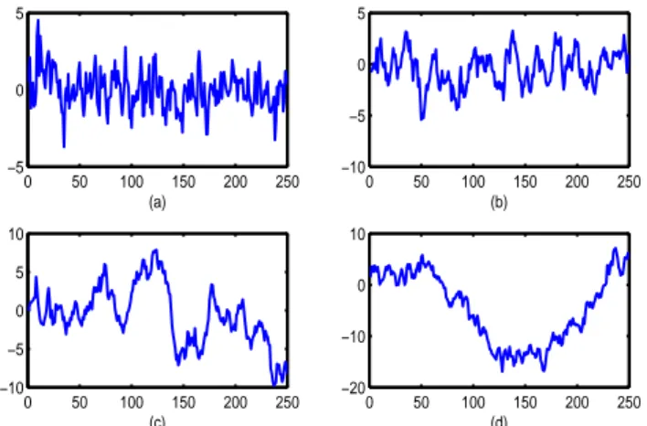
0 50 100 150 200 250 −5 0 5 (a) 0 50 100 150 200 250 −10 −5 0 5 (b) 0 50 100 150 200 250 −10 −5 0 5 10 (c) 0 50 100 150 200 250 −20 −10 0 10 (d)
Figure 1. Example of trajectories of a AR(1) process with: (a)ϕ = 0.50, (b) ϕ = 0.90, (d) ϕ = 0.95, (d) ϕ = 0.99.
Figure 1 displays some examples of trajectories of a stationary AR(1) process for some values of the parameter. The mean-reverting property appear clear from the figure. Furthermore, the absence of any kind of trends is more evident for small values of the autoregressive parameter. Stationarity assures that the mean,µ = E[Yt], and the variance, Vt2= Var(Yt), are
constants for all t. In particular, it is known thatµ = E[Yt]= 0 and Vt2= σ 2 ε
1−ϕ2 (see Hamilton (1994) for more details).
The autocovariance functionγk= E[(Yt− µ)(Yt−k− µ)], k = 1, 2, ... depends only on the lag k and it is given by
γk= σ 2 ε
1− ϕ2ϕ k,
whereas the autocorrelation function (ACF),ρk, has the form
ρk= γ k
γ0 = ϕ k.
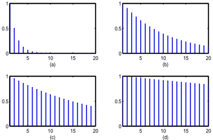
Notice that the ACF of a weakly stationary AR(1) process decays exponentially with rateϕ. Figures 2 shows the theoretical autocorrelation function for some values of the parameter. If the parameter assumes values close to 1 the decline of the ACF is much slower. For a detailed discussion on autoregressive processes we refer the reader to the manuals of Hamilton (1994) and of Brockwell and Davis (1991).
2.1 The Unit Root Case
In this paper we are particularly interested in the unit root case, i.e., when the autoregressive parameter ϕ = 1. The definition of a unit root process is the following.
Definition: 2. I(1). The discrete time stochastic process (Yt)t is called a unit root process, also known as integrated process, if
Yt= Yt−1+ εt,
where (εt)tis a white noise process. We denote such a process by I(1). Moreover, Yt−1is independent ofεt.
Observe that a unit root process is a random walk. As mentioned in the previous section, since the autoregressive parameter is equal to 1 the I(1) process is not stationary, as we can also infer by observing figure 3 which reports some simulated examples of paths of a unit root process. We can observe that the trajectories are not stationary in their means as we would expect if they were constant over time. As regards the variance, and more in general all higher-order moments, it depends on t. In particular, by repeated substitutions, we can write Yt = Y0+
∑t
5 10 15 20 0 0.5 1 (a) 5 10 15 20 0 0.5 1 (b) 5 10 15 20 0 0.5 1 (c) 5 10 15 20 0 0.5 1 (d)
Figure 2. Autocorrelation function of a AR(1) process with: (a)ϕ = 0.50, (b) ϕ = 0.90, (d) ϕ = 0.95, (d) ϕ = 0.99.
linearly with t Vt2 = t ∑ j=1 σ2 ε= tσ2ε,
and it approaches to infinity when t tends to infinity.
We can investigate the behavior of the state variable Ytand of its standard deviation Vtwith a Monte Carlo simulation. In
particular, we generate 5000 trajectories of 250 points of an I(1) process with initial condition Y0= 0 with the assumption
thatεtare i.i.d. N(0, σε); each simulated path (˜yt)t=1,...,250is a realization of the I(1) process, whereas if we fix t = t0we
have 5000 realizations of the state variable at the time t0, (˜y(i)t0)
i=1,...,5000.
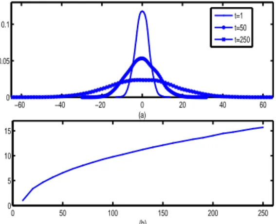
Figure 4 (panel (a)) reports the estimated probability density function relatively to (˜y(i)t )i=1,...,5000for increasing value of t.
We see that the dispersion of the distribution of ˜ytincreases as t increases, signalling that the process is not stationary in
variance. Moreover, figure 4 (panel (b)) displays the standard deviation, say ˜Vt, of a realization (˜y (i)
t )i=1,...,5000for increasing
values of t. As expected, ˜Vtis monotone increasing.
The theoretical autocorrelations of a I(1) process tend to one asymptotically for any lag k but the sample autocorrelations may decline rather fast even with large sample (Hassler, 1994). The average ACF up to the lag k = 20 over the 5000 simulated trajectories of our random experiment is reported in figure 5. Clearly, the inspection of this ACF is not sufficient to find out the presence of a unit root. A several test for the presence of unit roots are available in literature (Dickey, 1976; Dickey & Fuller, 1979; 1981).
0 50 100 150 200 250 −40 −30 −20 −10 0 10 20 30 t
Figure 3. Examples of trajectories of a unit root process.
3. The Convolution Based Unit Root Process
In this section we introduce a modified version of the standard unit root process based on the notion of C-convolution introduced by Cherubini, Mulinacci and Romagnoli (2011). The C-convolution was originally introduced to determine the distribution function of a sum of two dependent and continuous random variables X and Y. The dependence structure
−60 −40 −20 0 20 40 60 0 0.05 0.1 (a) t=1 t=50 t=250 0 50 100 150 200 250 0 5 10 15 (b)
Figure 4. (a) Probability density function of the state variable of a simulated unit root process; (b) Standard deviation of the state variable of a simulated unit root process
0 2 4 6 8 10 12 14 16 18 20 −0.2 0 0.2 0.4 0.6 0.8 Lag
Figure 5. ACF of an I(1) process.
between X and Y is modeled by a copula function. The copula technique allows to write every joint distribution as a function of the marginal distributions. In other words, we can represent the joint distribution of X and Y, say Pr(X ≤
a, Y ≤ b), with a, b ∈ R as a function of FX(a)≡ Pr(X ≤ a) and FY(a)≡ Pr(Y ≤ b). More formally, there exists a function CX,Y(u, v) such that
Pr(X≤ a, Y ≤ b) = CX,Y(FX(a), FY(b)). (1)
Conversely, given two distribution functions FX and FYand a suitable bivariate function CX,Y we may build joint
distri-bution for (X, Y). The requirements to be met by this function are that: i) it must be grounded (C(u, 0) = C(0, v) = 0); ii) it must have uniform marginals (C(1, v) = v and C(u, 1) = u); iii) it must be 2-increasing (meaning that the volume
C(u1, v1)− C(u1, v2)− C(u2, v1)+ C(u2, v2) for u1> u2and v1> v2cannot be negative).
The one to one relationship that results between copula functions and joint distributions is known as Sklar theorem. See Nelsen (2006) and Joe (1997) for a detailed discussion on copulas.
The C-convolution technique links the marginal distributions of X and Y and their dependence structure given by a copula so as to determine the probability distribution of the sum X+ Y. The seminal paper is that of Cherubini, Mulinacci & Romagnoli (2011) where we may find the concept of convolution-based copulas. If X e Y be two real-valued random variables with corresponding copula CX,Y and continuous marginals FX and FY, then the distribution function of the sum X+ Y, denoted by FX C ∗ FY, is given by FX+Y(z)= (FX C ∗ FY)(z)= ∫ 1 0 D1CX,Y ( w, FY(z− F−1X (w)) ) dw, (2) where D1CX,Y(u, v) denotes ∂CX,Y (u,v) ∂u .
The choice of the copula function affects the probabilistic behavior of the distribution of the sum (for a detailed discussion on this topic see the book of Cherubini, Gobbi, Mulinacci & Romagnoli (2012). Some of the most used copula functions
are the Gaussian copula, the Clayton copula, the Frank copula and the Gumbel copula. The Gaussian copula is constructed from a bivariate normal distribution overR2by using the probability integral transform. For a given correlation coefficient
ρ, the Gaussian copula with parameter ρ can be written as
C(u, v; ρ) = Φ2
(
Φ−1(u), Φ−1(v)),
whereΦ2is the bivariate standard normal distribution with correlation coefficient ρ and Φ is the standard normal
distribu-tion. The Clayton copula is an asymmetric Archimedean copula, exhibiting greater dependence in the negative tail than in the positive. Its functional form is given by
C(u, v; θ) = (u−θ+ v−θ− 1)−1/θ,
whereθ is the parameter which assumes positive values, θ ∈ (0, +∞). The Frank copula is a symmetric copula defined as
C(u, v; θ) = − ln
(
1+(exp(−θu) − 1)(exp(−θv) − 1) exp(−θ) − 1
) ,
where the parameterθ is a real number, θ ∈ R. The Gumbel copula is an asymmetric archimedean copula, exhibiting greater dependence in the positive tail than in the negative. This copula is given by:
C(u, v; θ) = exp
(
−((− ln u)θ+ (− ln v)θ)1/θ )
,
whereθ ∈ [1, +∞). It is important to notice that the C-convolution has a closed form if and only if the marginal distri-butions are gaussian and the copula linking them is the gaussian copula (see Cherubini, Gobbi, Mulinacci & Romagnoli, 2012). For computational purposes in this paper we only consider that case. The reader can find some examples of C-convolution with Clayton and Frank copulas in the book of Cherubini, Gobbi, Mulinacci & Romagnoli (2012).
Here, we are interested in how to use the C-convolution to modelling stochastic processes. As shown in Cherubini, Gobbi & Mulinacci (2016) we can construct a dependent increments Markov processes by a repeated application of the
C-convolution technique. More precisely, given a stochastic process (Yt)t, let Yt−1 with marginal distribution Ft−1and
∆Yt = Yt− Yt−1with distribution Ht. Moreover let C be the copula associated to (Yt−1, ∆Yt). Then, we may recover the
distribution of Yt= Yt−1+ ∆Ytiterating the C-convolution (2) for all t Ft(y)= (Ft−1 C ∗ Ht)(y)= ∫ 1 0 D1C ( w, Ht(y− Ft−1−1(w)) ) dw. (3)
The process (Yt)tis called the C-convolution based process. This methodology may be applied to define a new version of
the unit root process I(1), Yt= Yt−1+ εt, when Yt−1andεtare not independent as in the standard case but linked by some
copula C. This is our modified version of a I(1) process.
Notice that if the copula C is the independent copula, that is C(u, v) = uv, the C-convolution coincides with the standard convolution and we obtain the standard I(1) process. In this section we consider a C-convolution-based unit root process,
C-UR(1), by imposing a dependence structure between Yt−1andεt. The distribution of Yt = Yt−1+ εt is given by the
C-convolution between the distribution of Yt−1, Ft−1, and the distribution ofεt, Ht. Suppose that Y0has distribution F0.
Then, the distribution of Ytis
Ft(yt)= (Ft−1 C ∗ Ht)(yt)= ∫ 1 0 D1C(w, Ht(yt− F−1t−1(w)))dw, t = 1, 2, ... (4)
We are now ready to introduce the definition of our modified version of a I(1) process. In particular we have the following Definition: 3. C-UR(1). The discrete time stochastic process(Yt)tis a C-convolution based unit root process, C-UR(1), if
• the functional form is that of a unit root process, Yt= Yt−1+ εt;
• there exists a dependence structure between the state variable at the time t−1, Yt−1, and the innovationεt. Moreover, this dependence structure is described by a copula function, C, with a time-invariant parameter.
Remark 1. Patton (2005; 2006) introduced the notion of conditional copulas that allows us to define a time-varying
dependence structure. In other words, the parameter of the copula function depends on the time t while remaining within the same family of copulas.
3.1 The Gaussian C-UR(1) Process
As mentioned before, if C is not the gaussian copula the above integral (4) cannot be expressed in closed form and they have to be evaluated numerically. In those cases the simulation of a C-UR(1) process may not be simple. However, since the gaussian family is closed under C-convolution, we can perform a simulation design under some restrictions. In particular, suppose that the following conditions hold.
1. The initial distribution is gaussian:
Y0∼ N(0, σ0),
and the distribution of innovations is gaussian and stationary εt
i.i.d.
∼ N(0, σε).
2. The copula function linking Yt−1andεtis gaussian and stationary, i.e., C(u, v) = G(u, v; ρ), where ρ is the correlation
coefficient.
Under this framework, as shown in Cherubini, Gobbi & Mulinacci (2016), by iterating the C-convolution technique (4) we recover the distribution of the state variable for all t
Yt∼ N(0, Vt2), (5)
where the variance Vt2has a closed functional form
Vt2= Var(Yt)= V12+ (t − 1)σ 2 ε+ 2ρσε t−1 ∑ i=1 Vt−i, t = 1, ... (6)
Moreover, it is shown that the copula between two consecutive state variables, Yt−1and Yt, is Gaussian with parameters
ρXt−1,Xt =
Vt−1+ ρσε Vt
, t = 1, ..., where V1 = σ1.
Furthermore, we can prove that the behavior of V2
t when t→ +∞ depends on the correlation coefficient ρ. As shown in
Cherubini, Gobbi & Mulinacci (2016) the limiting behavior of the standard deviation Vtis
Vt−→
{ −σε
2ρ, if ρ ∈ (−1, 0);
+∞, otherwise. (7)
It is very significant to notice that the standard deviation of a C-UR(1) process does not grow indefinitely as t tends to infinity only in the case of negative correlation between Yt−1 andεt. Even more significant is the fact that the sufficient
condition isρ < 0. 4. Simulation Design
The simulation of a gaussian C-UR(1) process is based on the conditional sampling technique which allows to generate random pairs (u, v) from a given family of copulas (Nelsen, 2006 and Cherubini, Luciano & Vecchiato, 2004). The method is based on the property that if (U, V) are U(0, 1) distributed r.vs. whose joint distribution is given by C the conditional distribution of V given U= u is the first partial derivative of C
P(V ≤ v|U = u) = D1C(u, v) = cu(v),
which is a non-decreasing function of v. With this result in mind the simulation of a pair (u, v) from C is obtained in the following two steps. We call the following algorithm Alg1.
1. Generate two independent r.vs. (u, z) from a U(0, 1) distribution: (u, z)i.i.d.∼ U(0, 1).
2. Compute v= c−1u (z), where c−1u (·) is the quasi-inverse function of the first partial derivative of the copula. 3. (u, v) is the desired pair.
0 50 100 150 200 250 −20 −10 0 10 (b) 0 50 100 150 200 250 −20 0 20 (a) 0 50 100 150 200 250 −10 −5 0 5 10 (c)
Figure 6. Example of trajectories of a C-UR(1) process. (a)ρ = −5%; (b) ρ = −10%; (c) ρ = −25%.
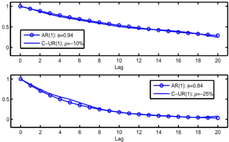
0 2 4 6 8 10 12 14 16 18 20 0 0.5 1 Lag 0 2 4 6 8 10 12 14 16 18 20 0 0.5 1 Lag AR(1): φ=0.94 C−UR(1): ρ=−10% AR(1): φ=0.84 C−UR(1): ρ=−25%
Figure 7. Comparison among autocorrelation functions of a standard AR(1) process and a C-UR(1) process with ρ = −10% (top) and ρ = −25% (bottom).
Now, we propose our algorithm to simulate trajectories from a C-UR(1) process using Alg1. The input is given by a sequence of distributions of innovations,εt, that for the sake of simplicity we assume stationary Ht = H and gaussian: H ∼ N(0, σε). Moreover we assume a dependence structure stationary and gaussian, CYt−1,εt(u, v) = G(u, v; ρ), We also
assume Y0= 0. We describe a procedure to generate a iteration of a n-step trajectory.
1. Generate u from the uniform distribution. 2. Compute ˜yt= H−1(u) with t= 1.
3. Use Alg1 to generate v from G(u, v; ρ). 4. Compute ˜εt+1= H−1(v).
5. ˜yt+1= ˜yt+ ˜εt+1.
6. Compute the distribution Ft+1by C-convolution given by equation (4).
7. Compute u= Ft+1(˜yt+1).
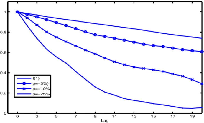
0 3 5 7 9 11 13 15 17 19 0 0.2 0.4 0.6 0.8 1 Lag I(1) ρ=−5%) ρ=−10% ρ=−25%
Figure 8. Comparison among autocorrelation functions.
0 50 100 150 200 250 0 1 2 3 4 5 6 7 8 9 10 t ρ=−5% ρ=−10% ρ=−25%
Figure 9. Standard deviation of the state variable of a simulated C-UR(1) process for three different values of the correlation coefficient.
We generate 5000 trajectories of 250 points. We can think of daily trajectories therefore 250 points refer to a calendar year. The number of trajectories has been chosen according to the computational resources available. Without loss of generality we setσε= 1 and we select three different levels of negative correlation: ρ = −5%, ρ = −10% and ρ = −25%.
4.1 Results
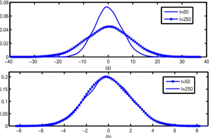
We now describe the results of our simulations. Figure 6 shows some simulated trajectories for each level of correlation. We can observe that as the correlation increases in absolute value the dynamics of trajectories appears more stationary both in mean and in variance. If we compare this figure with figure 3 the effect is even more clear. We notice a mean reverting effect which becomes stronger as the negative correlation increases. If we consider the autocorrelations the behavior of our C-UR(1) is also interesting. Table 1 reports the autocorrelation function for the first 20 lags for a I(1) process and for our C-UR(1) process with correlation level from -3% to -25%. The impact of negative correlation is clear. If in the case of low negative correlation the decline of autocorrelations is in fact identical (withρ = −3%) or very similar (withρ = −5%) to that of a I(1) process, when ρ is -10% or -25% the situation drastically changes. In particular, a negative correlation greater than -20% virtually eliminates serial correlation while being in the presence of a unit root. For example, in the case ofρ = −10% autocorrelations are very close to those of a standard AR(1) process with autoregressive parameterϕ around 0.94 whereas in the case of ρ = −25% are very similar to those of a standard AR(1) process with ϕ around 0.84 as we can see in figure 7. Figure 8 compares the dynamics of autocorrelations of a I(1) process with those of a C-UR(1) process with negative correlation from -5% to -25%. As regards the variance of the state variable, figures 9 and 10 show the impact of the negative correlation. More precisely, figure 9 reports the behavior of the standard deviation
Vt as a function of the time t. The convergence towards a constant level (given by equation 7) is faster as the negative
correlation increases. Ifρ = −25% the convergence to the limit value is immediate and the variance of the state variable is constant over time as in stationary processes. Figure 10 emphasizes this aspect showing that the dispersion is the same for
−400 −30 −20 −10 0 10 20 30 40 0.02 0.04 0.06 0.08 (a) −8 −6 −4 −2 0 2 4 6 8 0 0.05 0.1 0.15 0.2 (b) t=50 t=250 t=50 t=250
Figure 10. Panel (a). Probability density function of the state variable of a simulated C-UR(1) process withρ = −10%. Panel (b). Probability density function of the state variable of a simulated C-UR(1) process withρ = −25%.
both the instants of time considered ifρ = −25%. The linear relationship between the time t and the variance disappears. Table 1. Comparison among autocorrelation values for different choices of the correlation coefficient.
Lag I(1) ρ = −3% ρ = −5% ρ = −10% ρ = −25% 1 0.9836 0.9817 0.9756 0.9410 0.8633 2 0.9689 0.9637 0.9493 0.8699 0.7388 3 0.9520 0.9487 0.9227 0.8015 0.6317 4 0.9377 0.9373 0.8943 0.7502 0.5557 5 0.9241 0.9227 0.8653 0.7056 0.4955 6 0.9118 0.9096 0.8348 0.6649 0.4115 7 0.8970 0.8956 0.8030 0.6235 0.3342 8 0.8841 0.8813 0.7748 0.5851 0.2584 9 0.8718 0.8705 0.7569 0.5443 0.2084 10 0.8583 0.8589 0.7397 0.5079 0.1784 11 0.8456 0.8459 0.7208 0.4790 0.1443 12 0.8332 0.8321 0.7009 0.4556 0.1271 13 0.8190 0.8164 0.6807 0.4415 0.1115 14 0.8034 0.8022 0.6675 0.4284 0.0941 15 0.7882 0.7899 0.6576 0.4118 0.0818 16 0.7750 0.7788 0.6417 0.3879 0.0668 17 0.7630 0.7661 0.6276 0.3651 0.0500 18 0.7515 0.7548 0.6166 0.3311 0.0476 19 0.7395 0.7420 0.6075 0.2898 0.0558 20 0.7240 0.7261 0.5953 0.2449 0.0766 5. Conclusion
In this paper we propose a convolution based approach to the simulation of a modified version of a unit root process which we called C-convolution-based unit root process, C-UR(1). The idea is that once the distribution of innovations is specified, and the dependence structure between innovations and levels of the process is chosen, the distribution of the process can be automatically recovered. The variance of this new process converges to a constant level and this convergence is faster as the correlation becomes more negative. The autocorrelation function rapidly decay towards zero as soon as the correlation is around -20%. For these reasons, the model is well suited to address problems of persistent and unpredictable shocks, beyond the standard paradigm of linear models.
References
Econo-metric Theory, 4, 458-467. http://dx.doi.org/10.1017/S0266466600013396
Brockwell, P. J., & Davis, R. A. (1991). Time Series. Theory and Methods, Springer Series in Statistics. Springer-Verlag. http://dx.doi.org/10.1007/978-1-4419-0320-4
Chen, X., & Fan, Y. (2006). Estimation of copula-based semiparametric time series models. Journal of Econometrics,
130, 307-335. http://dx.doi.org/10.1016/j.jeconom.2005.03.004
Chen, X., Wu, W. B., & Yi, Y. (2009). Efficient Estimation of Copula-Based semiparametric Markov models. Annals of
Statistics, 37(6B), 4214-4253. http://dx.doi.org/10.1214/09-AOS719
Cherubini, U., & Gobbi, F. (2013). A Convolution-based Autoregressive Process, in F. Durante, W. Haerdle, P. Jaworski editors. Workshop on Copula in Mathematics and Quantitative Finance. Lecture Notes in Statistics-Proceedings. Springer, Berlin/Heidelberg. http://dx.doi.org/10.1007/978-3-642-35407-6 1
Cherubini, U., Luciano E., & Vecchiato, W. (2004). Copula Methods in Finance. London, John Wiley, (John Wiley Series in Finance). http://dx.doi.org/10.1002/9781118673331
Cherubini, U., Gobbi, F., & Mulinacci, S. (2016). Convolution Copula Econometrics. SpringerBriefs in Statistics. Cherubini, U., Mulinacci, S., & Romagnoli, S. (2011). A Copula-based Model of Speculative Price Dynamics in Discrete
Time, Journal of Multivariate Analysis, 102, 1047-1063. http://dx.doi.org/10.1016/j.jmva.2011.02.004
Cherubini U., Gobbi F., Mulinacci S., & Romagnoli S. (2012). Dynamic Copula Methods in Finance. John Wiley & Sons. Darsow, W. F., Nguyen, B., & Olsen, E. T. (1992). Copulas and Markov Processes, Illinois Journal of Mathematics, 36(4). Dickey, D. A. (1976). Estimation and hypothesis testing in non-stationary time series. (Unpublished doctoral
disserta-tion). Iowa State University, Ames, IA.
Dickey, D. A., & Fuller, W. A. (1979). Distribution of the estimators for autoregressive time series with a unit root,
Journal of the American Statistical Association, 74, 427-431.
Dickey, D. A., & Fuller, W. A. (1981). Likelihood ratio statistics for autoregressive time series with a unit root.
Econo-metrica, 49, 1057-1072. http://dx.doi.org/10.2307/1912517
Fama, E. F. (1965). Efficient Capital Markets: A Review of Theory and Empirical Work. Journal of Finance, 25(2), 383-417. http://dx.doi.org/10.2307/2325486
Hamilton, J. D. (1994). Time Series Analysis. Princeton University Press.
Hassler, U. (1994). The sample autocorrelation function of I(1) processes. Statistical Papers, 35, 1-16. http://dx.doi.org/10.1007/BF02926395
Joe, H. (1997). Multivariate Models and Dependence Concepts. Chapman & Hall, London. http://dx.doi.org/10.1201/b13150
Nelsen, R.(2006). An Introduction to Copulas. Springer.
Nelson, C., & Plosser, C. (1982). Trend and Randon Walk in Macroeconomic Time Series. Journal of Monetary
Eco-nomics, 10, 139-169. http://dx.doi.org/10.1016/0304-3932(82)90012-5
Patton, A. (2005). Modelling time-varying exchange rate dependence. International Economic Review, 47.
Patton, A. (2006). Estimation of multivariate models for time series of possibly different lengths. Journal of Applied
Econometrics, 21, 147-173. http://dx.doi.org/10.1002/jae.865
Samuelson, P. A. R. (1963). Proof That Properly Anticipated Prices Fluctuate Randomly. Industrial Management Review,
6, 41-50.
Samuelson, P. A. R. (1973). Mathematics of Speculative Price. SIAM Review, 15(1), 1-42. http://dx.doi.org/10.1137/1015001
Copyrights
Copyright for this article is retained by the author(s), with first publication rights granted to the journal.
This is an open-access article distributed under the terms and conditions of the Creative Commons Attribution license (http://creativecommons.org/licenses/by/4.0/).