Periodic, complex and kink-type solitons for the nonlinear model in microtubules

nonlinear model in microtubules

H. M. Baskonus, C. Cattani, A. Ciancio

Abstract. In this paper, we use the exponential function method to find

some complex travelling wave solutions in the nonlinear dynamics model which describes the dimer‘s dynamics within microtubules. We obtain some entirely complex and kink-type soliton solutions to this nonlinear model. By choosing some suitable values of parameters, we plot the vari-ous dimensional simulations of all the obtained solutions in this study. We observe that our result may be useful in detecting some complex waves behaviors of kink solitons moving along the microtubule

M.S.C. 2010: 35Axx; 35Exx; 35Sxx

Key words: The EFM; NLEEs; microtubules; periodic; complex; kink-type soliton

solutions; contour graphs.

1

Introduction

In recent several decades, many nonlinear evolution equations (NLEEs) for explain-ing more properties of Micro-Tubules (MTs) in solitons have been largely studied. Soliton theory plays an important role in the analysis of many nonlinear models that describe various phenomena in the field of nonlinear media. Dynamics of solitons has been largely studied in literature (see e.g. [1-3]). Moreover, powerful tools such as the exponential function method, the modified simple equation method,the Kudryashov method, Sumudu transform method, (G′/G)-expansion method and many more tech-niques have been used (see e.g. [4-12]). In this paper, we propose a soliton nonlinear model for the analysis of proteins. Proteins are indispensable part of living creatures. Major cytoskeletal proteins create Microtubules (MTs) [13]. These MTs are sketched as hollow cylinders usually formed by 13 parallel protofilaments (PFs) covering the cylindrical walls of MTs [13]. Each PFs symbolize a series of proteins called tubulin dimers [13-16]. S.Pospich et al have investigated an optimal tool to study cytoskeletal proteins [17]. P. Drabik et al and E. Nogales et al have studied on Microtube stability and high-resolution model of the Microtubule, and observed that the bonds between dimers within the same PFs are remarkable stronger than the soft bonds between neighbouring PFs [18,19]. This fact has been represented by the nonlinear dynamical equation (NDE) defined as [13,20].

A

(1.1) mΥtt(x, t)− kl2Υxx(x, t)− αΥ(x, t) + βΥ3(x, t) + γΥt(x, t)− qe = 0,

where Υ(x, t) symbolizes the real displacement of the dimer along x axis. This model is used to explain that the longitudinal displacements of pertaining dimers in a single PF should cause the longitudinal wave propagating along PF [13].

In this study, the exp (−φ(ζ))-exponential function method (EFM) will be used to find soliton solutions such as complex, dark and kink-type from the Eq.(1.1). Dark soliton describes the solitary waves with lower intensity than the background [21]. The kink-type soliton describes the physical properties of quasi-one-dimensional fer-romagnets [22] and the singular soliton solutions is a solitary wave with discontinuous derivatives; examples of such solitary waves include compactions [23,24]. In this sense, many powerful models along with engineering applications have been presented in lit-erature (see e.g. [29-33]).

2

The expansion function method (EFM)

Here, we shortly give the main steps of the EFM. Let us consider the nonlinear partial differential equation (NPDE):

(2.1) P (Ψ, Ψx, ΨxΨ2, Ψxx, Ψxxt, . . .) = 0,

where Ψ = Ψ(x, t) is the unknown function, and P is a polynomial in Ψ(x, t).

Step 1: By using the wave transformation:

(2.2) Ψ(x, t) = U (ζ), ζ = κx− ωt,

from Eq.(2.1), we obtain the nonlinear ordinary differential equation (NODE):

(2.3) N ODE(U, U′U2, U′, U′′, . . .) = 0,

where N ODE is a polynomial of U and its derivatives.

Step 2: Let us now assume the solutions of Eq. (2.3) to have the form:

(2.4) U (ζ) = n ∑ i=0 Ai [ e−φ(ζ) ]i = A0+ A1e−φ+ . . . + Ane−nφ,

where Ai, (0≤ i ≤ n) are constants to be obtained later, such that An ̸= 0, and

φ = φ(ζ) solves the following ODE:

Eq.(2.5) admits the following set of solutions [25, 26, 28, 29]: Set 1: When µ̸= 0, λ2− 4µ > 0, (2.6) φ(ζ) = ln ( −√λ2_{− 4µ} 2µ × tanh (√_λ2_{− 4µ} 2 (ζ + E) ) − λ 2µ ) . Set 2: When µ̸= 0, λ2− 4µ < 0, (2.7) φ(ζ) = ln (√ −λ2_{+ 4µ} 2µ × tan (√−λ2_{+ 4µ} 2 (ζ + E) ) − λ 2µ ) .

Set 3: When µ = 0, λ̸= 0 and λ2_{− 4µ > 0,}

(2.8) φ(ζ) =−ln ( λ eλ(ζ+E)− 1 ) .

Set 4: When µ̸= 0, λ ̸= 0 and λ2_{− 4µ = 0,}

(2.9) φ(ζ) = ln ( −2λ(ζ + E) + 4 λ2_{(ζ + E)} ) .

Set 5: When µ = 0, λ = 0 and λ2_{− 4µ = 0,}

(2.10) φ(ζ) = ln(ζ + E).

Ai, (0≤ i ≤ n), E, λ, µ are coefficients to be obtained, and n, m are positive integers

that one can find by the balancing principle.

Step 3: Inserting Eq.(2.4) together with its derivatives along with the Eq.(2.5) and

simplifying, we find a polynomial equation of e−φ(ζ). We extract a set of algebraic equations from this polynomial equation by summing the terms of the same power and equating each summation to zero. We solve this set of equations to find the values of the coefficients involved. By inserting the obtained values of the coefficients along with one of Eqs.(2.6-2.10) into Eq.(2.4), we can obtain the new solitons to the NPDE equation (2.1).

3

Application of EFM

In this section, we use the EFM to obtain some new solutions of the nonlinear dy-namical equation (1.1).

Consider the following travelling wave transformation:

Substituting Eq.(3.1) into Eq.(1.1), yields the following NODE; (3.2) (mω2− kl2κ2)Ψ′′− γωΨ′− αΨ + βΨ3− qe = 0.

Balancing the highest power nonlinear term and the highest derivative in Eq.(3.2). Doing so, the value of n is obtained as n = 1. Using n = 1 along with Eq.(2.4), yields

(3.3) Ψ(ζ) = A0+ A1e−φ,

Putting Eq. (3.3) along with its second derivative into Eq.(3.2), gives a polynomial equation in e−φ. We gather a group of algebraic equations from this polynomials by equating the sum of the coefficients of e−φ with the same power to zero. We solve this group of equations and obtain the values of the coefficients involved. To obtain the solutions of Eq.(1.1), we put the values of the coefficients into Eq. (3.3) along with Family-1 condition.

Case-1: A0= 3kl2_κ2_{λ− ω(γ + 3mλω)} 3√2√β√kl2_κ2− mω2 , A1= √ 2kl2_κ2− 2mω2 √ β , α = γ 2_ω2_{+ 3(λ}2_{− 4µ)(kl}2_κ2_{− mω}2₎2 6kl2_κ2− 6mω2 , q = γω(γ2ω2− 9(λ2− 4µ)(kl2κ2− mω2)2) 27√2e√β(kl2_κ2− mω2₎3₂ ,

with these coefficients, the following set of solutions are obtained:

Set-1: When µ̸= 0, λ2_{− 4µ > 0, Eq.(1.1) gives the following kink-type soliton}

solution:

(3.4)

Υ

(x, t) =

2µ

√

2ϖ

− λϱ

√

β

− ϱ

√

βϑtanh(

ϑ(e + κx

− ωt)))

−λ

√

β

− ϑ

√

βtanh(

ϑ(e + κx

− ωt))

,

where, ϖ = kl

_κ

_{− mω}

_,

_{ϑ =}

√

_λ

− 4µ, ϱ =

.

Figure 2: Contour plot of Eq.(3.4).

Set-2: When µ = 0, λ

̸= 0 and λ

_{− 4µ < 0, Eq.(1.1) is of the following}

periodic soliton solution:

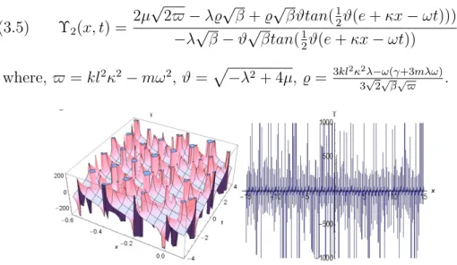
(3.5)

Υ

(x, t) =

2µ

√

2ϖ

− λϱ

√

β + ϱ

√

βϑtan(

ϑ(e + κx

− ωt)))

−λ

√

β

− ϑ

√

βtan(

ϑ(e + κx

− ωt))

,

where, ϖ = kl

κ

− mω

, ϑ =

√

−λ

_{+ 4µ, ϱ =}

.

Figure 3: The 2D and 1D (t=0.85 for 1D) surfaces of Eq.(3.5).

Case-2:

A

=

3qe(α + i

√

−9α

− 16γ

_µω

₎

4α

, A

=

−3eqγω

α

,

λ =

−

i

√

−9α

− 16γ

_µω

2γω

, m =

−2γ

3α

+

kl

κ

ω

, β =

4α

27e

_q

,

Figure 4: Contour plot of Eq.(3.5).

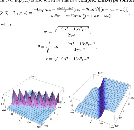
4µ > 0, Eq.(1.1) is also solved by this new complex kink-type soliton

(3.6)

Υ

(x, t) =

−6eqγµω +

(iϖ

− θtanh[

(e + κx

− ωt)])

iα

_ϖ

− α

_θtanh[

(e + κx

− ωt)]

,

where

ϖ =

√

−9α

− 16γ

_µω

2γω

,

θ =

√

−4µ −

−9α

− 16γ

µω

4γ

_ω

,

τ =

√

−9α

− 16γ

_µω

.

Figure 6: Contour plot of imaginary and real part of Eq.(3.6).

Figure 7: The 1D surfaces of imaginary and real part of Eq.(3.6) (t=0.85).

Case-3:A

=

√

, A

=

, λ =

√

, m =

+

, β =

27e2_q2

, with these coefficients, and, for F amily

− 1 with

µ

̸= 0, λ

− 4µ > 0, Eq.(1.1) is solved by the new complex kink-type

soliton

(3.7)

Υ

(x, t) =

−6eqγµω +

4

(qeα

− iqeτ)(−iϖ − θtanh[

θ 2

(e + κx

− ωt)])

α

₍

−iϖ − θtanh[

(e + κx

− ωt)])

,

where ϖ =

√

, θ =

√

−4µ −

, τ =

√

−9α

− 16γ

_µω

_.

Figure 8: The 2D surfaces imaginary and real part of Eq.(3.7).

Figure 9: Contour plot of imaginary and real part of Eq.(3.7).

4

Remark and comparisons

All analytical solutions obtained in this paper via EFM is completely new

with the results of [13], and has been introduced firstly to the literature

along with the figures plotted under the suitable values of parameters in

solutions.

5

Conclusion

In this paper, the exp (

−φ(ζ))-exponential function method has been

successfully used in extracting complex, kink-type and periodic singular

soliton solutions to the nonlinear dynamics model (1.1). The constraint

conditions for the existence of valid soliton solutions where necessary are

also given. The physical meaning of the obtained solutions in relations

to the nonlinear dynamics model (1.1) are given as well. Solutions (3.4),

(3,6) and (3.7) belong to complex and kink-type soliton solutions.

So-lution (3.5) belongs to periodic soliton soSo-lutions. The soSo-lution of Set-2

in Case-2 being λ

− 4µ < 0 is not valid because it is always positive as

λ

− 4µ =

> 0.

The soliton solutions obtained in this paper might be physically

use-ful in explaining how the bonds between dimers within the same PFs are

remarkable stronger than the soft bonds between neighbouring PFs. As

a physical aspects of results, it is observed that the hyperbolic tangent

arises in the calculation of magnetic moment and rapidity of special

rel-ativity [27]. The results found in here are entirely new when comparing

the results presented in [13]. To the best of our knowledge, the

applica-tion of EFM to the Eq.(1.1) has not been submitted to the literature in

advance. Finally, one can be inferred from results that the exp(

−φ(ζ))-exponential function method is a powerful and efficient mathematical

tool that can be used to find many soliton solutions such as complex,

kink-type and periodic to various nonlinear partial differential equations

with high nonlinearity.

Acknowledgement. This work was supported by National Group of

Mathematical Physics (GNFM-INdAM).

References

[1] D.W. Zuo, H.X. Jia and D.M. Shan, Dynamics of the optical solitons

for a (2+1)-dimensional nonlinear Schr¨

odinger equation,

[2] A.H. Arnous, S.A. Mahmood and M. Younis, Dynamics of optical

solitons in dual-core fibers via two integration schemes, Superlattices

and Microstructures 106 (2017), 156-162.

[3] M. Younis, H.U. Rehman, S.T.R. Rizvi and S.A. Mahmood, Dark

and singular optical solitons perturbation with fractional temporal

evolution, Superlattices and Microstructures 104 (2017), 525-531.

[4] M.A. Akbar and N.H.M. Ali, Exp-function method for duffing

equa-tion and new soluequa-tions of (2+1)-dimensional dispersive long wave

equations, Progress in Applied Mathematics 1, 2 (2011), 30-42.

[5] J.H. He and X.H. Wu, Exp-function method for nonlinear wave

equa-tions, Chaos, Soliton and Fractals 3, 3 (2006), 700-708.

[6] N. Kadkhoda and H. Jafari, Analytical solutions of the

Gerdjikov-Ivanov equation by using exp(

−φ(ξ))-expansion method,

Optik-International Journal for Light and Electron 139 (2017), 72-76.

[7] H. Jafari, N. Kadkhoda and A. Biswas, The (G

/G)-expansion

method for solutions of evolution equations from isothermal

mag-netostatic atmospheres, Journal of King Saud University-Science 25,

1 (2013), 57-62.

[8] M.M. Kabir and R. Bagherzadeh, Application of (G

/G)-expansion

method to nonlinear variants of the (2+1)-dimensional

Camassa-Holm-KP equation, Middle-East Journal of Scientific Research 9, 5

(2011), 602-610.

[9] M. Wang, X. Li and J. Zhang, The (G

/G)-expansion method and

travelling wave solutions of nonlinear evolution equations in

Mathe-matical Physics, Physics Letters A 372 (2008), 417-423.

[10] S. Guo, Y. Zhou and X. Zhao, The Extended (G

/G)-expansion

method and its applications to the Whitham-Broer-Kaup-Like

equa-tions and coupled Hirota-Satsuma KdV equaequa-tions, Applied

Mathe-matics and Computation 215 (2010), 3214-3221.

[11] H.L. Lu, X.Q. Liu and L. Niu, A generalized (G

/G)-expansion

method and its applications to nonlinear evolution equations,

Ap-plied Mathematics and Computation 215 (2010), 3811-3816.

[12] M.S. Islam, K. Khan and A.H. Arnous, Generalized Kudryashov

method for solving some (3+1)-dimensional nonlinear evolution

equations, New Trends in Mathematical Sciences 3, 3 (2015), 46-57.

[13] S.Zdravkovic, M. V. Sataric, S.Zekovic, Nonlinear dynamics of

mi-crotubules: a longitudinal model, ELP (A Letters Journal

Explor-ing), 102 (2012), 38002-38008.

[15] J.A. Tuszysky, S. Hameroff, M.V. Satari, B. Trpisov, M.L.A. Nip,

Ferroelectric behavior in microtubule dipole lattices: implications for

information processing, signaling and assembly/disassembly, Journal

of Theoretical Biology 174 (1995), 371-380.

[16] M.V. Satari, T.A. Tuszysky, Nonlinear dynamics of microtubules:

biophysical implications, Journal of Biological Physics 31 (2005),

487-500.

[17] S. Pospich, S. Raunser, Single particle cryo-EMan optimal tool to

study cytoskeletal proteins, Current Opinion in Structural Biology

52 (2018), 16-24.

[18] P. Drabik, S.Gusarov, A. Kovalenko, Microtubule stability studied by

three-dimensional molecular theory of solvation, Biophysical Journal

92 (2007), 394-403.

[19] E.Nogales, M. Whittaker, R.A. Milligan and K.H. Downing,

high-resolution model of the microtubule, Cell 96 (1999), 79-88.

[20] M.V.Sataric, J.A. Tuszynsky and R.B. Zakula, Kinklike excitations

as an energy-transfer mechanism in microtubules, Physical Review

E 48, 1 (1993), 589-597.

[21] A.C. Scott, Encyclopedia of Nonlinear Science, Routledge, Taylor

and Francis Group, New York, 2005.

[22] H.J. Mikeska and M. Steiner, Solitary excitations in one-dimensional

magnets, Advances in Physics 40, 30 (2006), 191-356.

[23] P. Rosenau, What is a compacton?, Notices of the American

Math-ematical Society 52, 7 (2005), 738-739.

[24] R. Camassa and D.D. Holm, An integrable shallow water equation

with peaked solitons, Physical Review Letters, 71 (1993), 1661-1664.

[25] Z. Lu and H. Zhang, Soliton like and multi-soliton like solutions for

the Boiti-Leon-Pempinelli equation, Chaos Solitons and Fractals, 19

(2004), 527-531.

[26] C.Dai and Y.Wang, Periodic structures based on variable separation

solution of the (2+1)-dimensional Boiti-Leon-Pempinelli equation,

Chaos, Solitons and Fractals, 39(2009), 350-355.

[27] E.W. Weisstein, Concise Encyclopedia of Mathematics, 2

_{d edition,}

CRC Press, New York, 2002.

[28] H.M.Baskonus and H.Bulut, Analytical studies on the

(1+1)-dimensional nonlinear dispersive modified Benjamin-Bona-Mahony

equation defined by seismic sea waves, Waves in Random and

Com-plex Media 25, 4 (2015), 576586,

[29] A.Ciancio, H.M.Baskonus, T.A.Sulaiman and H.Bulut, New

system with complex structure, Indian Journal of Physics, 92, 10

(2018), 1281-1290.

[30] T.A.Sulaiman, H.Bulut, A.Yokus and H.M.Baskonus, On the exact

and numerical solutions to the coupled Boussinesq equation arising

in ocean engineering, Indian Journal of Physics, 93, 5 (2019),

647-656.

[31] C. Cattani, T.A.Sulaiman, H.M.Baskonus and H.Bulut, Solitons in

an inhomogeneous Murnaghan’s rod, European Physical Journal Plus

133, 228 (2018), 1-12.

[32] S.H.Seyedi, B.N. Saray and M.R.H.Nobari, Using interpolation

scal-ing functions based on Galerkin method for solvscal-ing non-Newtonian

fluid flow between two vertical flat plates, Appl. Math. Comput. 269

(2015), 488-496.

[33] A.Yokus, H.M.Baskonus, T.A.Sulaiman and H.Bulut, Numerical

simulation and solutions of the two component second order KdV

evolutionary system, Numerical Methods for Partial Differential

Equations, 34, 1 (2018), 211-227.

Authors’ addresses:

Haci Mehmet Baskonus

Department of Mathematics and Science Education,

Faculty of Education, Harran University, Sanliurfa, Turkey.

E-mail: hmbaskonus@gmail.com

Carlo Cattani

Engineering School (DEIM), Tuscia University, Viterbo, Italy.

Ton Duc Thang University, Ho Chi Minh City, Vietnam.

E-mail: cattani@unitus.it

Armando Ciancio

Department of Biomedical and Dental Sciences and Morphofunctional Imaging

,

University of Messina, Messina, Italy.

E-mail: aciancio@unime.it