Analisys and Syntesys of Thin-Film Solar Cells with Metallic Nanoparticles

UNIVERSITA' DEGLI STUDI DI CATANIA

_____________________________________________

DOTTORATO DI RICERCA IN ENERGETICA

XXVI CICLO

VIVIANA CHIARELLO

ANALISYS AND SYNTESYS

OF THIN-FILM SOLAR CELLS

WITH METALLIC NANOPARTICLES

____________

TESI DI DOTTORATO

CONTENTS

 Preface...3

 Chapter 1 – The finite element method...4

- 1.1. The method

- 1.2. Discretization of the domain - 1.3. Scalar finite elements - 1.4. Vector finite elements

- 1.5. Building of the global algebraic system - 1.6. Solution of the global system

 Chapter 2 – Electromagnetic FEM analysis...23

- 2.1. The Maxwell's equations

- 2.2. Scattering of electromagnetic waves - 2.3. The FEM-RBCI method in 2D - 2.4. The FEM-RBCI method in 3D - 2.5. The perfectly matched layer (PML)

 Chapter 3 – Stochastic optimization...34

- 3.1. Generalities

- 3.2. Single- and multi-objective optimization - 3.3. Genetic algorithms (GAs)

- 3.4. Particle swarm optimization (PSO) - 3.5. Pattern search (PS).

 Chapter 4 – The photovoltaic conversion...45

- 4.1. Functioning principle of a photovoltaic cell - 4.2. The silicon structure

- 4.3. Semiconductor doping - 4.4. The p-n junction

- 4.5. Electrical characterization of a photovoltaic cell - 4.6. Efficiency of a photovoltaic cell

 Chapter 5 – Plasmonic resonances...54

- 5.1. Response models of the metals - 5.2. The Drude model

- 5.3. Volume plasmons - 5.4. Surface plasmons

 Chapter 6 – Numerical analysis of light scattering

from metal nanoparticles...61

- 6.1. Analysis of plasmons in metallic nanoparticles by FEM-RBCI

- 6.2. Numerical results

 Chapter 7 – Optimization of a solar cell with metal nanoparticles...70

- 7.1. Generality

- 7.2. 3D FEM analysis of light scattering from solar cells

-

7.3. Optimization by GAs

Preface

The interaction between electromagnetic radiation and condensed matter is a broad field of study concerning numerous practical applications in everyday life.

The metal nanoparticles have peculiar optical properties that determine a real revolution in the fields of physics, chemistry, materials science and bioscience, due to their ability to increase and to focus the electromagnetic fields in spatial regions smaller than the light wavelengths. This ability is due to the presence of localized surface plasmons (LSP), or collective undulatory excitations of free electrons in the metal particles. The manufacturing techniques bottom-up of plasmonic nanoparticles with high possibilities of control and precision are promising for the future construction of low-cost nanophotonic devices.

The plasmon science is enabling the development of a vast number of applications such as spectroscopy, high sensitivity, the realization of nanometric laser and of ultracompact optical circuities that is expected in the future can serve as an efficient bridge between the circuitry electronics and photonics. The surface plasmon intensity depends on many factors including the wavelength of the incident light and the morphology of the metal surface. The wavelength must be very close to that of the plasma of the metal. For particles of noble metals, such as silver and gold, this can fall in the visible region. This makes the interaction of these metals with the light particularly strong and leads to a highly dispersive permittivity at optical frequencies. In particular, the real part of the permittivity changes sign near the resonance frequency. For metal particles smaller than the skin depth, the plasmon interaction becomes a collective interaction that involves the entire nanoparticle. In practice, more interesting nanoparticles have diameters less than 100 nm. Among the noble metals, silver is the metal that has less absorption and produces more intense resonance effects. The number, the position and the intensity of the plasmon resonance depends on the geometric shape and size of the nanoparticle.

In this doctorate thesis we will see how to analyze numerically the surface plasmons of metal nanoparticles, and to optimally design a solar cell equipped with metal nanoparticles.

The structure of the thesis is the following. In Chapter 1 the finite element method (FEM) is briefly outlined, both in 2D and 3D geometries; in Chapter 2 the FEM analysis of electromagnetic scattering is described by means of the hybrid FEM-RBCI (Robin boundary condition iteration) and of the perfectly matched layer (PML) methods; in Chapter 3, two stochastic optimization methods are described, that is genetic algorithms (Gas) and particle swarm optimization (PSO); in Chapter 4 the photovoltaic conversion principles are recalled; in Chapter 5 the plasmon phenomena are briefly introduced; in Chapter 6 the numerical analysis of light scattering from metal nanoparticle is performed by means of FEM-RBCI method; in Chapter 7 a solar cell, equipped with metal nanoparticles, is optimized from the point of view of efficiency; finally the author's conclusions follow.

Chapter 1

The finite element method

1.1. The method

The solution of engineering problems makes use of mathematical models to represent physical situations. Within the framework of electrical and electronic engineering the behavior of these models can be described by partial differential equations, the well-known Maxwell's equations, to which are associated the corresponding initial and boundary conditions and the constitutive equations. The complexities of the analysis domains and / or of the constitutive equations make it impossible to obtain exact analytical solutions of these differential equations in most cases. So we often use numerical methods, which provide an estimate of the unknown quantities in a discrete and finite set of points of the domain. The values of these quantities in the other points are obtained by interpolating functions. The most widely used numerical methods are the finite difference method (FDM) and the finite element method (FEM).

The FEM [1-3] was born in the 60s and had a wide circulation as a result of the technological development of electronics and computers. It lends itself well to be implemented in computer programs, and can be used for a wide range of applications. These reasons have led to the success of this method compared to FDM, born before. The latter, although more simple and easy to implement, it is suitable to solve problems that have a high degree of complexity in the domain where there are no inhomogeneities and whose borders are well defined.

The FEM is based on the discretization of the domain of interest by means of a set of subdomains, said finite elements, of finite sizes and simple shapes, interconnected at points called nodes. The unknown values of the scalar field f (function of the spatial coordinates) are obtained from the nodal values fn (n=1,…,N) through appropriate interpolating functions αn

said form functions (or shape functions), defined within the finite elements:





 n n n (x,y,z) f ) z , y , x ( f (1.1.1)

Substituting this approximate expression in the differential equations that characterize the problem posed in an appropriate integral form, we obtain a system of algebraic equations in the unknown nodal values. These equations are linear or not, depending on the nature of the constitutive laws. The resolution of the system provides the unknown values fn and then the

approximate solution in the entire domain through the use of the shape functions.

1.2. Discretization of the domain

The first step of the numerical analysis is the finite element discretization of the domain, namely the creation of a mesh of finite elements, in which it was decided to subdivide the domain. Typical elements used for the solution of electromagnetic problems are the

simplexes, i.e. geometric entities having Nd + 1 vertices in a space of Nd dimensions (for

example, triangles in a two dimensional space and tetraheda in a three dimensional space). The choice of the element kind depends on the number of dimensions Nd of the problem and

on the shape of the domain. The use of a greater number of elements in a domain increases the accuracy of the solution, but causes an increase of the computational cost in terms of occupation of memory and computing time. A convenient approach is to increase the number of elements only where it is needed, i.e., where the unknown scalar field presents major changes. This can be done based on the experience of the user or automatically by means of algorithms of automatic adaptive meshing.

If we want a better approximation within a given finite element, it is necessary to give the approximate solution a greater number of degrees of freedom, in such a way as to reduce the difference between the approximate solution and the exact one. According to the Weierstrass theorem, given a function f(x), continuous in the closed and limited range [a, b], fixed an arbitrary number  > 0, there exists a polynomial p(x) such that:

f(x)p(x) x a,b It is clear that every continuous function can be approximated with the desired accuracy by a polynomial of sufficiently high degree. The type of simplest approximation is the linear one, but turns out to be the worst in terms of quality. In fact, the order of the polynomial used in the approximation of the real solution affects the accuracy with which we can evaluate the solutions of differential equations: the higher the grade, the better the approximation.

In Fig. 1.1 it is shown the basic principle used in the FEM method in the one-dimensional case: after having divided the domain of analysis in finite elements (in this case, intervals, typically having different amplitudes), we proceed to approximate the unknown function as in (1.1), choosing as unknowns only the values fn in the nodes of abscissas xn on the x-axis.

From the solution of a system of algebraic equations we obtain the approximate nodal values of the function f(x), while the values in the internal points are evaluated based on the approximation functions used. As we can deduce from the figure, the approximation would be better if the number of elements were increased or if higher-degree polynomials were chosen to approximate the function from one node to another.

f(x)

x

x

1

x

2

x

3

exact

…

x

n

…

f

n

f

1

f

2

f

3

f

N

approximate

x

N

1.3. Scalar finite elements

The electromagnetic problems in two dimensions (2D) can be always traced to scalar problems. This is achieved by assuming as unknown the electric scalar potential; alternatively the variable can be a component (along the z axis) of the magnetic vector potential, or directly of the electric or magnetic field.

The most used finite elements in 2D are the triangle and the quadrangle. Consider a triangular finite element E, defined by three vertices, Pn (xn, yn), n = 0,1,2, where you want to linearly

approximate a scalar field f(x, y). We have:

f(x,y) 2 f (x,y) P (x,y) E 0 n n n   



 (1.3.1)

where fn and n(x,y) are the nodal values and the shape functions, respectively. The shape

functions n(x,y) are non-dimensional linear functions, given by:

y A 2 x x x A 2 y y A 2 y x y x ) y , x ( n 1 n 2 n 2 n 1 n 1 n 2 n 2 n 1 n                (1.3.2)

They exhibit the property:        n m if 1 n m if 0 ) y , x ( _{m m} n (1.3.3)

In a domain D discretized with triangular finite elements, the umerical approximation of a scalar field f(x,y) is continuous in D.

It is useful to refer to the generic point P(x, y) of a finite element E in a reference frame ,, local to the element (Fig. 1.2 on the left), by means of the coordinate transformation:

                 ) y y ( ) y y ( y y ) x x ( ) x x ( x x 0 2 0 1 0 0 2 0 1 0 (1.3.4)

whose Jacobian is:

2A y y y y x x x x y y x x ) , ( J 0 2 0 1 0 2 0 1 _                    (1.3.5)

where A is the area of the finite element.

By means of (1.3.4), the finite element E is transformed into the standard triangle T, as shown in Fig. 1.2.

In local coordinates the shape functions simplify to:

y x P0 E   P1 P2   1 0 ₁ T P2 P1 P0

Fig. 0.2. - Triangular finite element of order 1 and standard triangle T.

The derivatives of the shape functions with respect to the absolute Cartesian coordinates are:

                                      n 0 1 n 0 2 n n 0 1 n 0 2 n A 2 x x A 2 x x y A 2 y y A 2 y y x (1.3.7)

By expressing the shape functions in the standard triangle T with the aid of the third local coordinate =1, we have:                                                   ) , , ( ) , , ( ) , ( ) , , ( ) , , ( ) , ( n n n n n n (1.3.8)

The three local coordinates , ,  can be interpreted as areolar coordinates in the element E; we have in fact: A A A A A A_{1 2 0}       (1.3.9)

where A0, A1 and A2 are the areas of the triangles obtained by joining the generic point P

inside the triangle with its vertices (see Fig. 1.3). It is clear that the sum of the three areolar coordinates is 1, ie: ++=1. y A0   P2 A1 P

y x P0 P1 P2 E P3 P4 P5   1 0 _1/2 T P1 1 1/2 P5 P2 P3 P0 P4

Fig. 0.4. - Triangular finite element of order 2 and standard triangle.

Triangular finite elements of higher order can be used. This choice increases the computational cost and the calculation time in favor of a better accuracy of the solution. For example, a finite element of the second order is shown in Fig. 1.4, with the associated standard triangle T. For this element the shape functions in local coordinates are:

                           4 4 4 ) 1 2 ( ) 1 2 ( ) 1 2 ( 5 4 3 2 1 0 _(1.3.10)

and the approximation of the scalar field is:

f(x,y) 5 f (x,y) P (x,y) E 0 n n n   



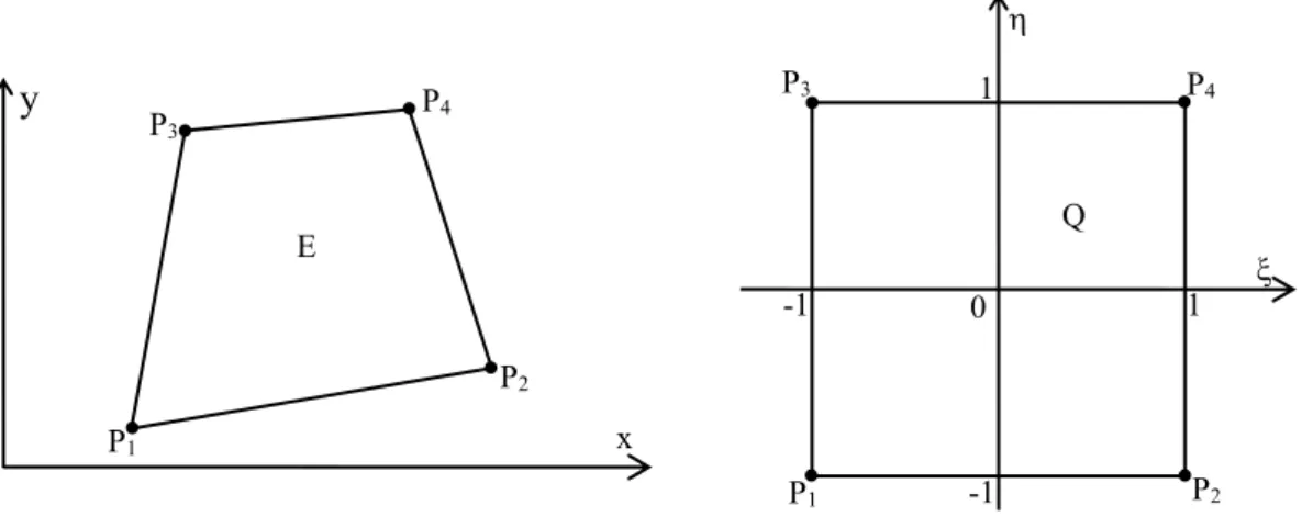
 (1.3.11)

In Fig. 1.5 a quadrangular finite element of order 1 is shown. By defining the local curvilinear coordinates ,, the shape functions are:

) 1 ( ) 1 ( ) 1 ( ) 1 ( ) 1 ( ) 1 ( ) 1 ( ) 1 ( 4 1 4 4 1 3 4 1 2 4 1 1                         (1.3.12)

and the coordinate transformations are:





          4 1 n n n 4 1 n n n ) , ( y y ) , ( x x (1.3.13)

These transformations transform the quadrangle E into the standard quadrangle Q (see Fig. 1.5). Note that the Jacobian of this transformation is not constant (exept for parallelograms), but it is a polynomial of degree 2 in the local coordinates.

The approximation of the scalar field is:

f(x,y) 4 f (x,y) P (x,y) E 1 n n n   



 (1.3.14)

y x P1 P2 P4 E P3   0 Q P1 P2 P3 P4 -1 -1 1 1

Fig. 0.5. - Quadrangular finite element of order 1 and standard quadrangle Q.

Some electromagnetic problems in three dimensions (3D) can be traced to scalar problems. This is the case of electrostatic and static current density problems formulated in terms of the scalar electric potential v.

The most used finite elements in 3D are the tetrahedron and the hexahedron. Consider a tetrahedral finite element E, defined by four vertices, Pn (xn, yn), n = 0,1,2,3 where you want

to linearly approximate a scalar field f(x, y, z). We have:

f(x,y,z) 3 f (x,y,z) P (x,y,z) E 0 n n n   



 (1.3.15)

where fn and n(x,y,z) are the nodal values and the shape functions, respectively. The shape

functions n(x,y,z) are non-dimensional linear functions:

_n(x,y,z)a_nxb_nyc_nzd_n (1.3.16) where le coefficients are

V 6 z y z y z y z y z y z y a_n  n1 n3 n2 n1 n3 n2 n1 n2 n2 n3 n3 n1 (1.3.17) V 6 z x z x z x z x z x z x b_n  n1 n2  n2 n3 n3 n1 n1 n3 n2 n1 n3 n2 (1.3.18) V 6 y x y x y x y x y x y x c_n  n1 n3 n2 n1 n3 n2 n1 n2  n2 n3 n3 n1 (1.3.19) V 6 z y x z y x z y x V 6 z y x z y x z y x d 2 n 1 n 3 n 1 n 3 n 2 n 3 n 2 n 1 n 1 n 2 n 3 n 3 n 1 n 2 n 2 n 3 n 1 n n                           (1.3.120)

In a domain D discretized with tetrahedral finite elements, the numerical approximation of a scalar field f(x,y,z) is continuous in D.

It is useful to refer to the generic point P(x,y,z) of a finite element E in a reference frame ,,, local to the element (Fig. 1.6 on the left), by means of the coordinate transformation:

                                   ) z z ( ) z z ( ) z z ( z z ) y y ( ) y y ( ) y y ( y y ) x x ( ) x x ( ) x x ( x x 0 3 0 2 0 1 0 0 3 0 2 0 1 0 0 3 0 2 0 1 0 (1.3.22)

whose Jacobian is:

6V y y z z z z y y y y y y x x x x x x z z z y y y x x x ) , ( J 0 3 0 2 0 1 0 3 0 2 0 1 0 3 0 2 0 1                                        (1.3.23)

where V is the volume of the tetrahedral finite element.

By means of (1.3.22), the tetrahedral finite element E is transformed into the standard tetrahedron T, as shown in Fig. 1.6. In local coordinates the shape functions simplify to:

                             ) , , ( ) , , ( ) , , ( 1 ) , , ( 3 2 1 0 _(1.3.24)

and the shape function derivatives with respect to the absolute Cartesian coordinates are:

                                    n 0 1 0 2 0 2 0 1 n 0 3 0 1 0 1 0 3 n 0 2 0 3 0 3 0 2 n V 6 ) z z ( ) y y ( ) z z ( ) y y ( V 6 ) z z ( ) y y ( ) z z ( ) y y ( V 6 ) z z ( ) y y ( ) z z ( ) y y ( x (1.3.25)                                     n 0 1 0 2 0 2 0 1 n 0 1 0 3 0 3 0 1 n 0 3 0 2 0 2 0 3 n V 6 ) z z ( ) x x ( ) z z ( ) x x ( V 6 ) z z ( ) x x ( ) z z ( ) x x ( V 6 ) z z ( ) x x ( ) z z ( ) x x ( y (1.3.26

                                    n 0 1 0 2 0 2 0 1 n 0 3 0 1 0 1 0 3 n 0 2 0 3 0 3 0 2 n V 6 ) y y ( ) x x ( ) y y ( ) x x ( V 6 ) y y ( ) x x ( ) y y ( ) x x ( V 6 ) y y ( ) x x ( ) y y ( ) x x ( z (1.3.27)

By expressing the shape functions in the standard triangle T with the aid of the fourth local coordinate =1, we have:                                                                                     ) , , , ( ) , , , ( ) , , ( ) , , , ( ) , , , ( ) , , ( ) , , , ( ) , , , ( ) , , ( n n n n n n n n n (1.3.21)

The four local coordinates , , ,  can be interpreted as volume coordinates in the element E; we have in fact: V V V V V V V V_{1 2 3 0}         (1.3.22)

where V0, V1, V2 and V3 are the volumes of the four tetrahedra obtained by joining the

generic point P inside the tetrahedron with its four vertices. It is clear that the sum of the four volume coordinates is 1, ie: +++=1.

y z x P0 P1 P2 P3    E    P3 P0 P1 P2 T 1 1 1 0

1.4. Vector finite elements

The electromagnetic problems in 3D are very often vector problems, in which the unknowns are vector fields instead of scalar ones. The representation of such vector fields by means of three scalar fields exhibits several drawbacks:

 It imposes the continuity of the three components of the vector at the interface between two adjacent finite elements; this is not true if the two elements are constituted of different materials with different constitutive parameters;

 The imposition of the boundary conditions are difficult;

 The numerical solutions exhibit errors (spurious modes), whose amplitude is not controllable.

For all such reasons, vector finite elements have been devised, named edge elements. In the edge elements the shape functions are of vector kind. The most used edge elements are the triangle and the quadrangle in 2D, and the tetrahedron and hexahedron in 3D. Other elements (more rarely) used are the prism with triangular base and the pyramid with quadrangular base. It is possible to show that a generic finite volume can be subdivided in tetrahedra, but this is not true for hexahedra, prisms and pyramids.

By indicating the four local coordinates , , ,  in a tetrahedron by i, i=0,…,3, the generic

edge shape function is:

_ijL_ij(_i_j_j_i) (1.4.1) were indices i=1,…3 and j=i+1,…,4 are relative to the beginning and ending nodes of the edge, oriented from node i to node j, as shown in Fig. 1.7. Said eˆ_ij the versor of the edge ij, it can be shown that:

eˆ_ij_kh _ik_jh (1.4.2) where  is the Kronecker delta. In other words, the vector shape functions (1.4.1) are interpolating vector functions. These shape functions ensure the continuity of the tangential components of the vector field, but not the normal components. Therefore this kind of finite element is very useful for electromagnetic problems where the unknown field is the electric field or the magnetic one, whose tangential components are continuous across the interface between two different materials.

By numbering the edges of the tetrahedron from 1 to 6 as shown in Fig.1.7, the electric (or magnetic) field inside the tetrahedron is approximated as:



   6 1 s s s (x,y,z) E ) z , y , x ( E  (1.4.3)

where the six degrees of freedom Es s=1,…,6 are relative to the mean values of the tangential

component of the field along the edge s:





 s e s s _L1 E tˆdl E  (1.4.4)

where tˆ is the versor of the edge es and Ls its length.

Note that in literature several ways exist to extend the tetrahedral edge element to higher orders.

y

z

x P0 P1 P2 P3 1 2 3 4 5 6

Fig. 0.7. - Tetrahedral edge element.

For a hexahedron of the first order the degrees of freedom are the average values of the tangential component of the vector field along the edges of the element, for a total of 12 unknowns, as shown in Fig. 1.8.

The vector shape functions of a hexahedral finite elements are:

                                                                                                ) 1 )( 1 ( ) 1 )( 1 ( ) 1 ( ) 1 ( ) 1 ( ) 1 ( ) 1 ( ) 1 ( ) 1 ( ) 1 ( ) 1 )( 1 ( ) 1 ( ) 1 ( ) 1 ( ) 1 ( ) 1 )( 1 ( ) 1 ( ) 1 ( ) 1 )( 1 ( 8 L 12 8 L 6 8 L 11 8 L 5 8 L 10 8 L 4 8 L 9 8 L 3 8 L 8 8 L 2 8 L 7 8 L 1 11 3 12 6 10 4 9 5 8 2 7 1             (1.4.5)

and the electric (or magnetic) field inside the hexahedron is approximated as:



   12 1 s s s (x,y,z) E ) z , y , x ( E  (1.4.6) y

z

P3 P8 2 9 4 6 5 P5 P₄ P6 P7 3 7 ₈ 10 11 12

1.5. Building of the global algebraic system

The FEM requires that the problem is formulated in terms of a functional,. whose minimization is equivalent to the solution of the partial differential equation with the associated boundary conditions. Consider the partial differential equation:

Lf g in D (1.5.1) where L is a differential linear operator, f is an unknown scalar function and g is a known

function (source). Assume that the function f satisfies the following Dirichlet and Neumann boundary conditions:           ) Neumann ( on 0 n f ) Dirichlet ( on f f Neu Dir d (1.5.2)

where fd is a known function defined on a subset Dir of the boundary  of the domain D, and

Meu is such that:

_dir _neu  _dir _neu  (1.5.3) It can be shown that the solution of the problem minimizes the functional [2]

        





dir d D D 2 1 on f f dxdydz f g dxdydz f f ) f ( min L (1.5.4)

Having discretized the domain D by means of nodal finite elements of a given order, the unknown scalar field f can be represented as a linear combination of shape functions and nodal values: f(x,y,z) f (x,y,z) [f_tot]t[ _tot] N 1 n n n tot    



 (1.5.6)

where Ntot is the total number of nodes in the finite element mesh, fn are the nodal values and

the n the relative shape functions. The array [ftot] and [tot] are the column vectors of the

nodal values and of the shape functions, respectively; the superscript t denotes transposition. Without loss of generality, we can number first the Nint internal nodes, after the Nneu nodes on

the Neumann boundary neu, and finally the Ndir nodes on the Dirichlet boundary dir. The

number of unknowns N is given by:

NN_intN_neu (1.5.7) By using the approximation (1.5.6), the functional becomes:



 



      _{ }   D tot t tot tot D t tot tot t tot 2 1 dxdydz g ] [ ] f [ ] f [ dxdydz ] [ ] [ ] f [ ) f ( L (1.5.8)

which can be put in matrix form as:

_tot t



_tot



_{tot tot} t

 

_tot

2 1 g ] f [ ] f [ A ] f [ ) f (    (1.5.9) where:

- [Atot] is the matrix of the coefficients, whose generic entry is:

a





dxdydz

D m n n m

2 1

mn



 L  L (1.5.10)

- [gtot] is an array, whose generic entry is:

g gdxdydz

D m

m 



 (1.5.11)

Now we can partition the arrays [ftot] as

_       ] f [ ] f [ ] f [ d tot (1.5.12)

This partition induces similar partitions in the matrix [Atot] and in the array [gtot], so that

_                                 ] g [ ] g [ t ] f [ ] f [ ] f [ ] f [ ] A [ t ] A [ ] A [ ] A [ ] f [ ] f [ ) f ( d d d dd d d t d 2 1 _(1.5.13)

where we have assumed that the matrix [Atot] is symmetric; this is a very common case and is

verified if the differential operator L is self adjoint. By expanding (1.5.13), we get:

               

  

d dd

         

d t d t d 2 1 t d d 2 1 d 2 1 2 1 g f g f f A t f f A t f f A t f f A t f ) f ( _d         (1.5.14) By noting that

          

f t A_d f_d  f_d t A_d t f (1.5.15) we can rewrite (1.5.14) as:

           





  

     



1₂ d dd d d t d



d d 2 1 g f f A t f g f A t f f A t f ) f (        (15.16)

0 f_n    n=1,2,…,N (1.5.17) or in matrix notation:

_{ }

 

 

         

A f A f g 0 f f d d       (1.5.18) By setting:

      

b A_d f_d  g (1.5.19) we obtain the global algebraic system of N equations in N unknowns:

    

A f  b (1.5.20) Another approach, which leads to the same global system, is the Galerkin method. By this method the partial differential equation (1.5.1) is rewritten in homogeneous form, multiplied by a shape function n and then integrated over the whole domain:

( f g) dxdydz 0

D  n 



L n=1,…,N (1.5.21) By substituting to f its approximation (1.5.6), we obtain the global system (1.5.21) again. The Galerkin method is more general than the functional approach, since it can be applied also in the cases in which the functional does not exist, as, for example, in the solution of skin effect problems by means of the integrodifferential Konrad's equation.

1.6. Solution of the global system

The methods of solution of linear algebraic equations are classified as direct and iterative solvers.

The direct solvers perform a finite number of operations, which depends on the order of the matrix, in general O(N3). Such methods obtain an exact solution in exact arithmetic, and no truncation error is introduced.

The iterative solvers are based on repeated corrections of an approximate solution; they introduce a truncation error and, in general it is not possible to foresee a priori the number of steps needed.

The direct methods are used only for systems of limited number of unknowns (some thousands). If the matrix is banded, symmetric and positive defined (SPD) it is possible to solve greater systems (some tens of thousands). Since the FEM linear systems are very big, in general iterative solvers are used.

Consider the linear algebraic system:

[A][x][b] (1.6.1) where [A] is a square matrix and [b] the known term array. We intend to use an iterative solver to solve (1.6.1) for [x]. Let [y] be an approximate solution, previously computed. We define the error:

[e][x][y] (1.6.2) Since the solution [x] is unknown, also the error [e] is unknown, but it is possible to compute the residual:

[r][A][e][A][x][A][y][b][A][y] (1.6.3) By using the approximate solving method by which we have computed [y], we obtain another approximation [e'] for [e]:

[e'][A]1[r] (1.6.4) We set:

[y'][y][e'] (1.6.5) By repeating this procedure, more good solutions are found. Now it is necessary to specify the algorithm by which to build such approximate solutions. Since this algorithm is applied repeatedly, it needs to be fast in the building of the approximate solutions.

We decompose the matrix [A] as:

[A][D][L][U] (1.6.6)

where [D] is the diagonal of [A], and [L] and [U] are the lower and upper triangular parts of [A]. The linear system is rewritten as:

[D][x]



[L][U]



[x][b] (1.6.8) and also:

[x][D]1



[L][U]



[x][D]1[b] (1.6.9) From this we have the following iterative scheme (Gauss-Jacobi) [4]:

[y(n)][D]1



[L][U]



[y(n1)][D]1[b] (1.6.10) If [y(n)]=[x] at the nth step, then [y(m)]=[x] for all the subsequent steps m>n. This iterative scheme fall within the general case described above. In fact we have:









] r [ ] D [ ] y [ ] b [ ] D [ ] y [ ] A [ ] D [ ] y [ ] b [ ] D [ ] y [ ] U [ ] L [ ] D [ ] D [ ] D [ ] b [ ] D [ ] y [ ] U [ ] L [ ] D [ ] y [ 1 ) 1 n ( 1 ) 1 n ( 1 ) 1 n ( 1 ) 1 n ( 1 1 ) 1 n ( 1 ) n (                             (1.6.11)

Obviously the algorithm which finds fast the approximate solutions is the diagonal system having [D] as matrix of coefficients.

Consider now another iterative scheme (Gauss-Seidel) [4]:

[y(n)]



[D][L]



1[U][y(n1)]



[D][L]



1[b] (1.6.12) If [y(n)]=[x] at the nth step, then [y(m)]=[x] for all the subsequent steps m>n. This iterative scheme fall within the general case described above.











 

















[D] [L]



[r] ] y [ ] b [ ] L [ [ D [ ] y [ ] A [ ] L [ ] D [ ] y [ ] b [ ] L [ [ D [ ] y [ ] U [ ] L [ ] D [ ] L [ ] D [ ] L [ ] D [ ] b [ ] L [ ] D [ ] y [ ] U [ ] L [ ] D [ ] y [ 1 ) 1 n ( 1 ) 1 n ( 1 ) 1 n ( 1 ) 1 n ( 1 1 ) 1 n ( 1 ) n (                                    (1.6.13)

The linear system which is solved to obtain the approximate solutions is the system having [D][L] as matrix of coefficients.

The two methods are convergent if their iteration matrices, that is [D]1([L]+[U]) for the Gauss-Jacobi solver and ([D][L])1[U] for the Gauss-Seidel one, have spectral radii less than 1. It possible to show that the Gauss-Jacobi method converges if the matrix [A] è strictly diagonal dominant, whereas the Gauss-Seidel converges if [A] is SPD. Note that such conditions are sufficient but not necessary.

This two methods in general converge slowly, so that very often another method, called the conjugate gradient (CG) is used [4].

Consider the linear algebraic system (1.6.1) and assume that [A] is a square matrix of order N, symmetric and positive definite. The solution of such a system can be seen as the minimization of the function:

g([x]) [x]t[A][x] [x]t[b]

2

1 _

 (1.6.14)

Having defined the residual as in (1.6.3) in relation to an approximate solution, the conjugate gradient algorithm is described in the following.

0) the counter k is initialized: k=0

1) given the initial approximate solution [x(0)], the initial residual and direction are computed:

[r(0)][A][x(0)][b] [p(0)][r(0)] (1.6.15) 2) the function g([x]) is minimized along the straight line through the point [x(n)] and having the direction [p(n)]. In other words, the function g()=g([x(n)] +  [p(n)]) is minimized with respect to the real parameter . The minimum is obtained for the parameter value:

] p ][ A [ ] p [ ] r [ ] p [ ) n ( t ) n ( ) n ( t ) n ( n   (1.6.16)

3) a new approximate solution is found as:

[x(n1)][x(n)]_n[p(n)] (1.6.17) 4) and the relative residual is

[r(n1)][r(n)]_n[A][p(n)] (1.6.18) 5) a new search direction is set:

[p(n1)][r(n1)]_n[p(n)] (1.6.19) with: ] p ][ A [ ] p [ ] r ][ A [ ] p [ ) n ( t ) n ( ) 1 n ( t ) n ( n     (1.6.20) 6) the counter k is increased by 1: k=k+1;

7) the convergence is tested:

_   2 ) 1 n ( 2 ) 1 n ( ] x [ ] x [ ] x [ 100 ) n ( (1.6.21) where  is a user-selected small values;

8) if the test is positive, the algorithm stops; otherwise it goes back to step 2). Note that the minimization is performed on the quadratic function:



 

 



] r [ ] p [ ] p [ ] A [ ] p [ ) ] x [ ( g ] b [ ] p [ ] x [ ] p [ ] x [ ] A [ ] p [ ] x [ ]) p [ ] x ([ g ) ( g ) n ( t ) n ( ) n ( t ) n ( 2 2 1 ) n ( t ) n ( ) n ( ) n ( ) n ( t ) n ( ) n ( 2 1 ) n ( ) n (                    (1.6.22)

from which it is easy to find the (1.6.16). Moreover, from (1.6.16) it follows that:

_n[p(n)]t[A][p(n)][p(n)]t[r(n)]0 (1.6.23) and also:

[p(n)]t



_n[A][p(n)][r(n)]



0 (1.6.24) and by virtue of (1.6.18):

[p(n)]t[r(n1)]0 (1.6.24) that is [p(n)] and [r(n+1)] are orthogonal.

Finally, note that, by imposing that two consecutive residuals are orthogonal, we have:

[r(n)]t[r(n1)][r(n)]t[r(n)]_n[r(n)]t[A][p(n)]0 (1.6.25) and so: ] p ][ A [ ] r [ ] r [ ] r [ ) n ( t ) n ( ) n ( t ) n ( n   (1.6.26)

which coincides with the (1.6.16). By setting:

[p(n)][r(n)]_n1[p(n1)] (1.6.27) we note that the numerators in (1.1.16) and (1.6.26) are the same:

] r [ ] r [ ] p [ ] r [ ] r [ ] r [ ] p [ ] r [ ) n ( t ) n ( ) 1 n ( t ) n ( 1 n ) n ( t ) n ( ) n ( t ) n (      _  (1.6.28)

If we impose that two successive directions are conjugate with respect to the matrix [A], that is

[p(n1)][A][p(n)]0 (1.6.29) one obtains that:

] p ][ A [ ] p [ ] r ][ A [ ] p [ ) n ( t ) n ( ) 1 n ( t ) n ( n     (1.6.30)





] p ][ A [ ] r [ ] p ][ A [ ] p [ ] p [ ] A [ ] r [ ] p [ ] A [ ] p [ ] r [ ] p [ ] A [ ] p [ ) n ( t ) n ( ) n ( t ) 1 n ( 1 n ) n ( t ) n ( ) n ( t ) 1 n ( 1 n ) n ( ) n ( t ) n (              (1.6.31)

References Chapter 1

[1] O. C. Zienkiewicz and R. I. Taylor, The Finite Element Method, McGraw-Hill, Maidenhead, 1991.

[2] P. P. Silvester and R. L. Ferrari, Finite Elements for Electrical Engineers, Cambridge University Press, Cambridge, 1990.

[3] J. M. Jin, The Finite Element Method in Electromagnetics, Wiley, New York, 1993. [4] G. H. Golub and C. F. Van Loan, Matrix Computations, John Hopkins Univ. Press,

Chapter 2

Electromagnetic FEM analysis

2.1. The Maxwell's equations

In order to solve problems of propagation of electromagnetic wave, it necessary to solve the Maxwell's equations in time-harmonic behavior [1,2]:

divD  (2.1.1) div B 0 (2.1.2)

rotE jB (2.1.3)

rotH JjD (2.1.4) were =2f is the angular frequency (rad/s) and f the frequency (Hz), E is the electric field (V/m), H the magnetic field (A/m), J the current density (A/m2), D the electric induction (C/m2), B the magnetic induction (Wb/m2), and  the volume charge density (C/m3).

These vector fields are related by the constitutive laws, which describe the media in which they are located:

D E (2.1.5) BH (2.1.6) JE (2.1.7) where  is the electric permittivity (F/m),  the magnetic permeability (H/m) and  the electric conductivity (S/m).

In addition to these equations, it is necessary to impose the boundary conditions.

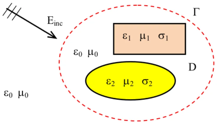
In the solution of the problems of scattering of electromagnetic waves, an incident wave E_inc

(or H_inc), analytically known, irradiates one or more non-homogeneous objects in a surrounding homogeneous unbounded medium, very often the vacuum, characterized by

m / S 0 m / H 10 4 m / F 10 8541878 . 8 0 7 0 12 0            (2.1.8)

0 0 2 2 2 1 1 1 Einc 0 0 D 

Fig. 2.1. Electromagnetic wave incident on non homogeneous objects.

2.2. Scattering of electromagnetic waves

A plane incident wave is given by [2]:

_E_incEmaxejk0(nxxnyynzz) _(2.2.9) where nx, ny and nz are the cosines of the wave propagation direction.

The scattered electromagnetic wave E_scat (or H_scat), due to the presence of the objects, is superimposed to the incident one to obtain the total electric field:

E E_inc E_scat (2.2.10) which satisfies the Helmholtz's equation:





_rE



k2₀'_rE0 (2.2.11) where r is the relative reluctivity (r=1/r ), 'r is the relative complex permittivity given by:

0 r r j '       (2.2.12)

and k0 is the free-space wavenumber:

k₀  ₀₀ (2.2.13) The boundary conditions, to be imposed on the boundaries of the analysis domain, are the following:

 on the perfect conductors (PEC):

 on the symmetry planes of the electric field:

nˆrotE 0 (or nH 0) (2.2.16)  on the far fictitious boundaries:

nˆE_scatjk₀nˆ(nˆE_scat)0 (2.2.17) In order to use the FEM, the unbounded free space outside the scatterers must be truncated by means of a fictitious truncation boundary F. The resulting bounded domain is discretized by

tetrahedral edge elements. By applying the Galerkin method to the Helmholtz equation (2.2.11), we have:



( E) k ' E



dxdydz 0 D r i 2 0 r       



   i=1,..,N (2.2.18)

where _i is the vector shape function of the i-th edge and N is the number of edges not lying on the Dirichlet boundary. By applying the first Green formula to (2.2.18), we get:

dS E nˆ dxdydz E ' k dxdydz E i r D r i 2 0 D r i                    







       i=1,2,..,N (2.2.19)

where  is the boundary of the analysis domain and nˆ the outward normal versor to the boundary. By substituting to the electric field its approximation:



   e N 1 j j j (x,y,z) E ) z , y , x ( E  (2.2.20)

the following element matrix must be computed: 



  k E j i ) k ( ij dxdydz s   (2.121) 



  k E j i ) k ( ij dxdydz t   (2.2.22) for each finite element Ek.

Finally, by imposing the boundary conditions, we obtain the global algebraic system.

Electromagnetic scattering problems can be posed also in 2D. This happens in if the wave is E- or H-polarized along a given direction, say the z axis, and all objects are cylinders aligned along the same axis. In such cases, assumed as unknown the polarized field along the z axis, the problem becomes scalar. In the case of E-polarized wave, the incident wave is:

_{Einc Emaxe}jk0(nxxnyy) _(2.2.23) and the Helmholtz's equation becomes:

k ' E 0 x E y x E x r 2 0 r r                           (2.2.24)

with the boundary conditions E=0 on the perfect conductors (Dirichlet), E/n=0 on the symmetry planes (Neumann) and Escat/n+jk0Escat=0 on the truncation boundary. By

discretizing the analysis domain by means of nodal finite elements (triangles and/or quadrangles), the Galerkin method gives:



( E) k ' E



dxdy 0 D r i 2 0 r       



i=1,2,…,N (2.2.25)

where i is the scalar shape function of the i-th node and N is the number of nodes not lying

in the Dirichlet boundary. By virtue of second Green formula, the (2.2.25) is rewritten as:







              dl n E dxdy E ' k dxdy E _{r i} D r i 2 0 D r i i=1,2,…,N (2.2.26)

where  is the boundary of the analysis domain D and nˆ is the outward normal versor to . By substituting to the electric field its approximation:



   N 1 j j j (x,y) E ) y , x ( E (2.2.26)

and by imposing the boundary conditions, we obtain the global system. In order to derive these equations, we have to compute the following geometrical coefficients [1]:





  k E j i ) k ( ij dxdy s (2.2.27) 



  k E j i ) k ( ij dxdy t (2.2.28) for each finite element Ek in the mesh. The coefficients (2.2.27) and (2.2.28) form the

stiffness and metric matrices of the finite element, respectively.

2.3. The FEM-RBCI method in 2D

Let us consider a set of conducting and/or dielectric objects, infinitely extended in the z-direction, surrounded by an unbounded homogeneous dielectric medium (free space). A given time-harmonic electromagnetic wave Einc, E-polarized along the z-axis irradiates these objects, so that a scattered field Escat is excited extending to infinity. The total field E(x,y)

(given by Einc+Escat outside the dielectric objects, if any) satisfies the two-dimensional scalar

and ₀ are the free-space magnetic permeability and electrical permittivity, respectively. Homogeneous Dirichlet conditions hold on the perfectly conducting scatterer surface C, if

any. In addition the scattered field Escat satisfies the Sommerfeld radiation condition at infinity.

Let us introduce a fictitious boundary F enclosing all the scattering objects. Note that this

boundary does not need to be constituted by a single closed curve, but several closed curves can be used, each one, for example, enclosing one scattering object. A Robin boundary condition is initially imposed on such a boundary [3-5]:

jk₀E on _F n E E        (2.3.2)

where the normal derivative is computed in the outward direction and  is a user-selected function of the position on the fictitious boundary (a good initial choice for  is given by Einc). By applying the Galerkin method to the bounded domain D, delimited by F and C

and discretized by means of Lagrangian finite elements, the following algebraic system is obtained:

A Ε CΨ _(2.3.3)

where A is a square matrix depending on geometry and dielectric materials, E is the array of the unknown nodal field values (including that on F),  is the array of the nodal values of

the right hand-side of the Robin condition on F and C is a rectangular matrix.

Consider now the total field outside the surface enclosing the scatterer and enclosed by F,

with a nonzero distance between them. The total field outside S is given by:



 _               S s d n G E n E G E E _inc (2.3.4)

where n is the outward normal to S (toward F), and G is the two-dimensional free-space

Green's function, given by [2]:

G jH(₀2)

 

k₀r

4 1



 (2.3.5)

where H ₀2 is the Hankel function of the second kind and zero-order and r is the distance between a point on S and a point on F. Owing to the fact that F and S are separated by a

distance greater than zero, function  can then be expressed as:



 _                    M s d n G E G n E inc . (2.3.6)

In the FEM approximation, this relation is rewritten as:

ΨΨ_incME _(2.3.7)

where inc is the vector of the values of the operator  applied to the incident field on the

nodes of the fictitious boundary and M is a rectangular matrix in which null columns appear for the nodes not belonging to the elements external to S and having a side lying on it.

System (2.3.3) will be referred to as the FEM part of the equations, while (2.3.7) will be referred to as the integral part of the equations.

Equations (2.3.3) and (2.3.7) form an algebraic system, which can be efficiently solved with the following iterative scheme:

a) having arbitrarily guessed the vector , b) equation (3) is solved for the vector E;

c) another guess for the Robin condition on F is obtained by means of (2.3.7);

d) the procedure is then iterated until convergence takes place.

The convergence is checked by computing the norm of the difference between the solution at the current step with the previous one, and dividing this quantity by the norm of the current solution; when this ratio is less than the convergence tolerance selected by the user the iteration is stopped.

A simple study of the convergence of this iterative procedure can made led by formally relating the initial guess (0) _{to the true values of the Robin condition t by means of the} error Ψ(_e0):

Ψ(0) Ψ_t Ψ(_e0) (2.3.8) Solving equation (2.3.3) for the vector E, we obtain the field solution at the 0-th step:

E(0) A1CΨ_tA1CΨ(_e0) (2.3.9) in which the first term gives, by definition, the true field solution E_t, whereas the second one represents the error E(_e0). Starting from this solution, the new guess for the Robin condition on F is computed, whose error is given by:

Ψ(_e1) PΨ(_e0) (2.3.10) where P is a square matrix (of order equal to the number of nodes on _F) given by:

PMA1C. (2.3.11) By further continuing the procedure, we can generalize (10) for the n-th step:

Ψ(_e1)PnΨ(_e0). (2.3.12) From this relation it is easy to understand how the procedure may converge to the true solution for every initial error Ψ(_e0)on the first guess for . This happens if and only if the spectral radius  of matrix P is lower than 1. In this case, in fact, Pn0 as n and, consequently, Ψ(_en)0 whatever Ψ(_e0). If this condition does not apply, divergence may occur.

the procedure is rapidly convergent to the true solution. This very attractive behavior of the procedure is lost if one tries to employ Dirichlet (or Neumann) boundary conditions on the fictitious boundary as is successfully done for static and quasi-static field problems for two reasons: equation (2.3.1) may have non vanishing solutions satisfying homogeneous boundary conditions; if there exist an incident field vanishing on _F then equation (2.3.4) is singular. On the contrary, with the use of an impedance condition, system (2.3.3) which constitutes the FEM part of the system cannot be singular. The way in which the singularity relative to the integral equation (2.3.6) is avoided is a little more involved. In the global system (2.3.3),(2.3.7) the known term is constituted by the array inc in equation (2.3.7); it results

from the discretization of Einc which vanishes if and only if Einc vanishes, so that this array

is zero if, and only if, the incident wave is zero. In other words, the field source is well represented in the formulation.

Finally, some comments are in order about the computing time and memory requirements of the procedure. At first sight one could think that the procedure is too time- consuming. In reality this is not the case if the following points are fully exploited in implementation.

i) Since the FE mesh remains unchanged through the various iteration steps, matrices A, M and C do not change, so that they are computed only once, at the beginning of the procedure and saved for further use.

ii) Equation (2.3.3) may be solved efficiently by means of standard solvers, which exploit the matrix A sparsity and symmetry. Specifically, when a direct solver is used, matrix A must be decomposed only once (note that in the adaptive ABC described in [8] matrix A changes at each step, so that the use of a direct solver may become too time- consuming); when an iterative solver is used the FEM solution at a certain step is used as the initial guess for the next step, reducing the number of solver iterations.

iii) Small extensions of the domain D can be obtained by suitably placing the fictitious boundary near the scattering objects. The distance between the fictitious boundary and the scatterer surface is very short with respect to that necessary to find an acceptable solution by ABC methods. In addition, if the fictitious boundary is constituted by several closed curves, each one enclosing a scattering object, the domain is subdivided into disjoint pieces and, consequently, the global FEM system (2.3.3) is partitionable into independent subsystems, with a reduction in the overall computing time.

iv) The end-iteration test is conveniently restricted to the fictitious boundary, as suggested by (2.3.12), being sure that this assures convergence of the field solution in the domain.

v) A good initial guess for (0) is inc since the number of iterations are minimized (note that

the selected Robin operator  looks like an ABC one).

By implementing all the above items the iterative procedure can be made competitive with respect to other techniques as far as computing time and memory requirements are concerned. In addition the procedure is easy implementable in a pre-existing FEM code for bounded problems. Only one routine has to be developed which calculates the matrix M entries (very often a similar routine is already available in the post-processing program). Note that no singularities arise in these calculations since _F and _S do not have points in common.

2.4. The FEM-RBCI method in 3D

Consider a set of conducting and/or dielectric bodies, embedded in free space, lit up by an incident time-harmonic electromagnetic wave. A scattering problem is set up in terms of the total electric field, which satisfies the 3-D vector Helmholtz equation (a time factor ejt has been assumed and suppressed):



E



k2 _rE 0 0 1 r         _(2.4.1) where r is the relative magnetic permeability, r the relative electrical permittivity and k0 is

the free-space wavenumber k₀ (₀₀)1/2, in which  is the wave angular frequency and 0 and 0 are the free-space magnetic permeability and electrical permittivity, respectively. Homogeneous Dirichlet conditions ( nˆE0) hold on the perfectly conducting scatterer surface C, if any. In addition the scattered field Escat satisfies the Sommerfeld radiation

condition at infinity.

Let us introduce a closed fictitious boundary F, strictly enclosing the scatterer, as shown in

Fig. 2.1. Note that when the scatterer is composed of several disjoint objects, the boundary can be constituted by several closed surfaces, each one, for example, enclosing a single object. On F, a nonhomogeneous Robin boundary condition is assumed [6-7]

EnˆEjk₀nˆ(nˆE)U (2.4.2) where nˆ is the outward normal to F and U is an unknown vector to be determined.

Let us now discretize the bounded domain delimited by F and by C by means of edge

elements such as first-order tetrahedra, whose vector shape functions are [1]

_i L_i



_i1_i2_i2_i1



(2.4.3) where i1 and i2 are the local coordinates relative to the two nodes of the i-th edge and Li is

its length. To simplify the description of the FE formulation and without loss of generality, we number first the edges on from one to, next the interior edges from NF+1 to N, and finally

the edges on C.

Applying FEM to (2.4.1) inside D with a homogeneous Dirichlet condition on C and a

boundary condition (2.4.2) on F, a linear algebraic system is obtained

AE BU (2.4.4) where A is a complex and symmetric matrix, B links (2.4.2) with the right hand side of the FEM system, E is the array of the expansion coefficients for the electric field , and U is the array whose generic entry is given by:



   F dS U U_j _j (2.4.5) Since U is unknown, in order to solve the scattering problem, another equation relating U to E needs to be derived. To this end let us now consider another surface, M, lying between the

antenna and the fictitious boundary (see Fig. 2.1). At minimum this surface can be selected as coinciding with the scatterer surface itself. The total field outside M can be expressed as:

 



_











 









M ' dS ) ' r ( E ' nˆ ) ' r , r ( g ) ' r ( E ' ' nˆ ) ' r , r ( G ) r ( E ) r ( E _inc (2.4.6)

_{0 e} jk0r r' ' r r 4 1 ) ' r , r ( g      (2.4.8)

Taking the curl of (2.4.6) and performing some manipulations, the following expression is obtained:















            M ' dS ) ' r ( E ' ' nˆ ) ' r , r ( g ) ' r ( E ' nˆ ) ' r , r ( G k ) r ( E ) r ( E _inc 2₀ (2.4.9)

Note that in (2.4.9), the curl operator has been put inside the integral sign due to the fact that F and M do not intersect. Substituting (2.4.6) and (2.4.9) in (2.4.2), an integral expression

for U is easily obtained. Then taking into account (2.4.5), the following algebraic equation is derived:

UU_incQE (2.4.10) where U_inc is an array whose generic j-th entry (j=1,…NF) is given by



    F dS E U_inc,j _inc _j (2.4.11)

and Q is an NFN rectangular matrix in which null columns appear for the internal edges not

involved in the computation. Equations (2.4.4) and (2.4.10) together form the global algebraic system of the FEM-RBCI method, which can be conveniently solved by an iterative scheme as follows:

1) Select an arbitrary first guess for U;

2) Solve equation (2.4.4) for E, by means of a standard conjugate gradient solver (COCG); 3) Obtain an improved guess for U by means of (2.4.10);

4) If the procedure has converged, stop; otherwise go to 2).

This scheme can be seen as a two-block Gauss-Seidel iterative method:

E(n) A1BU(n) (2.4.11)

U(n1) U_incQE(n) (2.4.12)

In this way the symmetry and sparsity of matrix A is fully exploited. Moreover, since this procedure converges in a few iterations (generally 10-20), it also minimizes the number of multiplications of the dense matrix Q by a vector. It is now clear now that the price paid by FEM-RBCI in meshing some space around the conductors is worth it. In fact if a similar approach were used in FEM-BEM, one would have to invert the sub-matrix relative to the unknowns on the truncation boundary with a computational complexity of O(N3)

F . On the

other hand, if an iterative solver for non-symmetric complex matrices were be directly applied to the solution of the FEM-BEM global system the dense BEM sub-matrix would be multiplied by a vector at each solver iteration. Since the number of such iterations is very high (from several hundreds to some thousands for big 3D problems) we can state that the RBCI global system is cheaper to solve than the BEM one. Another advantage of FEM-RBCI with respect to FEM-BEM is that it avoids singularities in the integral equation since, as already said, the integration surface M is different from the truncation one F.

The FEM-RBCI method can be made computationally more efficient if: a) the fictitious boundary is selected in such a way that very small extensions of the domain D are obtained: in general one or two layers of finite elements can be inserted between the scatterer and the

fictitious boundary; b) the computational complexity of the integral equation (2.4.9) is reduced from O(N2)

F to O(NFlogNF) by means of the well-known fast multipole method

(FMM) [9].

2.5. The perfectly matched layer (PML)

In dealing with electromagnetic problems in open boundaries, it is necessary to truncate the computational domain by means of a fictitious truncation boundary. The key question is how to do this without introducing significant errors in the model of the device to be tested. Some electromagnetic field problems by their own nature are confined in a specific region of space. Others present solutions that decay quickly in space, making irrelevant the error introduced by the truncation, if the computational domain is large enough. The problems regarding wave propagations, whose solutions oscillate and typically decay slowly, are the most complicated to truncate. Methods such as the simple truncation of the domain (using homogeneous Dirichlet or Neumann conditions) or the coordinate transformations would cause reflection invalidating the solution found.

In 1994 Berenger presents a new method [10]: instead of imposing a boundary condition that absorbs the wave, he uses a layer of artificial material that does not reflect the incident fields on it. The relative dielectric constant and the relative magnetic permeability of the material are both anisotropic. This material is a sort of picture frame for domain along the direction in which you want to simulate the open space (see Fig. 2.2); on the external surface of the adsorbing layer a Dirichlet boundary condition is imposed. When the electromagnetic field meets the absorbing layer, the amplitude of the wave decays exponentially; thus, in the case where the wave reaches the Dirichlet condition and is reflected, it must again pass through the absorbing layer, resulting largely attenuated and therefore negligible. This method takes the name of Perfectly Matched Layer (PML).



₀



₀



2



2



2



₁



₁



₁

D

References Chapter 2

[1] P. P. Silvester and R. L. Ferrari, Finite Elements for Electrical Engineers, Cambridge University Press, Cambridge, 1990.

[2] J. M. Jin, The Finite Element Method in Electromagnetics, Wiley, New York, 1993. [3] S. Alfonzetti, G. Borzì, and N. Salerno, "Iteratively-improved Robin boundary

conditions for the finite element solution of scattering problems in unbounded domains", Int. J. Num. Meth. Engng, vol. 42, pp. 601-629, 1998.

[4] S. Alfonzetti, G. Borzì, and N. Salerno, "Accelerating the Robin iteration procedure by means of GMRES", Compel, vol. 17, pp. 49-54, 1998.

[5] S. Alfonzetti, G. Borzì, and N. Salerno, "An iterative solution to scattering from cavity-backed apertures in a perfectly conducting wedge", IEEE Trans. Magn., vol. 34, pp. 2704-2707, 1998.

[6] S. Alfonzetti, B. Azzerboni, and G. Borzì, "Numerical computation of antenna parameters by means of RBCI", Electromagnetics, vol. 22, pp. 381-392, 2002.

[7] S. Alfonzetti, and G. Borzì, "Finite element solution to electromagnetic scattering problems by means of the Robin boundary condition iteration method", IEEE Trans. Ant. Prop., vol. 50, pp. 132-140, 2002.

[8] Y. Li and Z. Cendes, "High-accuracy absorbing boundary conditions", IEEE Trans. Magn., vol. 31, pp. 1524-1529, 1995.

[9] N. Engheta, W. D. Murphy, V. Rokhlin, and M. Vassiliou, “The Fast Multipole Method for Electromagnetic Scattering Computation,” IEEE Trans. Ant. Prop., vol. 40, pp. 634-641, 1992.

[10] J. P. Berenger, "A perfectly matched layer for the absorption of electromagnetic waves", J. Comput. Phys., vol. 114, pp. 185-200, 1994.

Chapter 3

Stochastic Optimization

3.1. Generalities

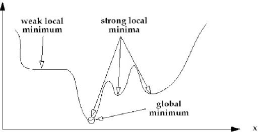
The aim of an optimization problem is to find the value of some design parameters in order to minimize (maximize) a given quantity, called objective function. Moreover, the optimization problem can be subject to some restrictions (constraints) on the parameter ranges allowed. In industrial applications, the optimized design is often problematic because of the simultaneous occurrence of many conflicting objectives. Besides, in optimised design it is often preferred to have a wide range of solutions to choose from, taking into account further design factors (cost, feasibility, …), instead of only considering the best one. There are different methods to solve this kind of problem, such as optimizing a single multi-objective function obtained by a weighted sum of the objectives or finding multiple Pareto-optimal solutions.

Many multi-objectives evolutionary algorithms exist in the literature but they can be extremely expensive. This is especially harmful in the design of electromagnetic devices, where each estimation of the objective function calls for a numerical solution of the electromagnetic problem by means of the Finite Element Method (FEM).

In this thesis, two stochastic optimization algorithms are presented: the Genetic Algorithms (GAs) and the Particle Swarm Optimization (PSO). Moreover, the Pattern Search (PS) deterministic algorithm is used to further improve the optima obtained by GAs and PSO. This chapter is structured as follows. In section 3.2 the concepts of single-objective and multi-objective optimization are introduced and an overview of well-known evolutionary algorithms is presented. In sections 3.3 and 3.4 the Gas and PSO are outlined, respectively, whereas in section 3.5 the PS is briefly described.