Analysis of linear networks with inconsistent initial conditions

IEEE TRANSACTIONS ON CIRCUITS AND SYSTEMS-I: FUNDAMENTAL THEORY AND APPLICATIONS, VOL. 40, NO. 12, DECEMBER 1993 885

Circuits and Systems Expositions

Analysis

of

Linear Networks with

Inconsistent Initial Conditions

Javier Tolsa and Miquel Salichs

Abstract-This paper presents a new method to analyze time- invariant linear networks allowing the existence of inconsistent initial conditions. This method is based on the use of distributions and state equations. Any time-invariant linear network can be analyzed. The network can involve any kind of pure or controlled sources. Also, the transferences of energy that occur at t=O are determined, and the concept of connection energy is introduced. The algorithms are easily implemented in a computer program.

I. INTRODUCTION

NITIAL conditions may be inconsistent when there occurs

I

a change in the network topology, as when two capacitors with different initial voltages are connected in parallel to form a new network.

The instant when a network forms a new topology will be

t = 0. Initial conditions at 0- will be called initial conditions simply, while the values immediately after switching are the initial conditions at O+. This paper will show an efficient and simple method to analyze an electric network knowing the initial conditions at 0-.

Voltage and current values at O+ and 0- are related by charge conservation in capacitive cutsets and flux conservation in inductive loops. Nevertheless, the application of these laws does not always suffice for obtaining the initial values at O+ from initial values at 0-: in the network of the second example of Section VIII, there is only one inductor, and its flux at 0- is different from its flux at Of.

Consider the two capacitors again. If initial voltages are different, the total energy stored in capacitors at O+ is smaller than the energy at 0- because at

t

= 0, the capacitors have transformed part of their energy stored in their electric field into electric energy, which is not zero if initial conditions are inconsistent. This energy, which we call the connection energy, is analyzed in detail in this paper.

The problem of determining initial values at O+ has been studied before. However, the analysis of the electric energy

Manuscript received February 20, 1992; revised manuscript received March 20, 1993. The work of J. Tolsa was supported by the Department d'Ensenyament de la Generalitat de Catalunya under Grant DOGC n. 1514,

6.1 1.1991. This paper was recommended by Associate Editor S . Karni. The authors are with the Department d'Enginyeria Elhctrica, Universitat Polithcnica de Catalunya, Barcelona 08028, Spain.

IEEE Log Number 9210020.

absorbed in the network connection is a little studied subject that this paper treats in detail.

Dervisoglu [3] developed an algorithm to calculate initial

values at Of using a state variable approach. His method does not involve distributions directly, but introduces the Dirac impulse

S

and its derivatives in the analysis. Murakami [4] pro- posed another way of determining the response of a network with inconsistent initial conditions. However, his method does not allow the existence of dependent sources and pure current sources. His analysis is based on the state equation and the use of distributions, although the application of distributions is not as interesting as in our new formulation. Recently, Opal and Vlach [ 5 ] proposed a new method to calculate initial values at O+ without introducing state equations. They use a numerical Laplace transform inversion, exact for impulses and its derivatives. In their algorithm, it is necessary to integrate a system of equations in a time interval At tending to zero.

This fact introduces numerical errors difficult to measure. The problem of conservation of energy when initial con- ditions are inconsistent has been studied by Goknar [12]. He considers networks consisting of capacitors or inductors only, without sources. He demonstrates that in those networks, the difference of the energy stored in capacitors (or inductors) from 0- to O+ is always positive, and that this difference equals the energy consumed in the interval [0, +cc[ by some resistors properly included into the network. However, he does not explain why the principle of conservation of energy seems to be violated.

Our approach is based on currents and voltages defined as distributions. The method is simple: first, equations of the network (Kirchhoff's laws and Ohm's law) are stated for currents and voltages defined as distributions. Then, we obtain a singular system of differential equations of distributions. This system is similar to classic singular systems of differential equations for functions, which can be written as

d dt

where the matrix T may be singular. Next, this equation is

transformed into the following pair of equations:

S Y ( t )

+

T - Y ( t ) = E ( t )

886 IEEE TRANSACTIONS ON CIRCUITS AND SYSTEMS-I: FUNDAMENTAL THEORY AND APPLICATIONS, VOL. 40, NO. 12, DECEMBER 1993 Switches are not considered as elements of the network. Instead, we assume that the network topology for t 2 0 is different from the topology for t

<

0.

Our approach to the problem of energy is very different from [12]. Our analysis is valid for any linear time-invariant network, including controlled and uncontrolled sources. We will study the transferences of energy, and we will find out why the total energy stored in inductors and capacitors at 0- is different from that of O+.

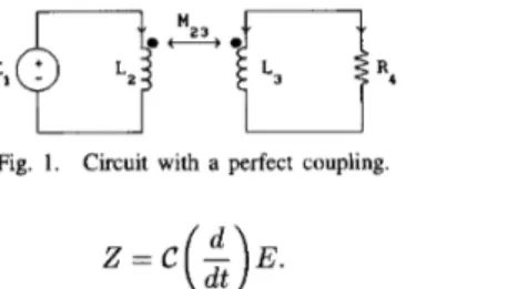
Fig. 1. Circuit with a perfect coupling.

Z=C(-$E. (2)

Then, state equation (1) is solved by the convolution of

distributions. 11. PRELIMINARIES

In our analysis, the matrix

B

need not be constant, although there always exists a state equation where

B

is constant. This is derived immediately from the theory of polynomial matrices and the Kronecker form exposed by Gantmacher [ 1 11,

which Verghese [lo] uses in his analysis of singular systems. However, sometimes the computation of

B

in this formulation is very difficult.

To illustrate these different choices for the matrix

B,

con- sider Fig. 1, with L2 = L3 = M23 = L (the coupling is perfect and the order of the circuit is one). We derive

The concept of distribution [6] generalizes the concept of function. A distribution is defined as a continuous linear map from the space of all C" real functions with compact support into CG. Locally integrable functions can be considered as a particular case of distributions. Any distribution is infinitely derivable. The set of distributions is a vector space which is denoted by

D'.

It is always possible to consider the restriction of a distri- bution to an open set (similar to the restriction of a function to an open set). Nevertheless, not all distributions defined in

d d _{an open set can be extended to the whole of R.}

dt dt In an electrical network, distributions that define currents

d d _{and voltages depend only on time. To define the values of}

d t dt distributions at 0-, we suppose that there exists an interval

]

- e, O[, 6

>

0 such that the restriction of those distributions to this interval is a continuous function such that its limit exists at 0-. If f is such a distribution and

f

is defined in

] . - e, +ea[, it is easy to demonstrate that

f

can be written in a unique way as follows:

L-I2

+

L-I3 = El

L-I2

+

L--I3 = -R413.

If we choose I2

+

I3 as the state variable, the state equation is

d 1

~

(

+

1 3 )

4

= - E l .

L

SO A is zero and

23

is constant. On the other hand, if I2 is the state variable, we obtain

d 1 1 d

f = f - + f +

-I2 = -El

+

---El.

d t L R4 dt

where

f-

is the restriction of

f

to the interval

]

- E, O [

(extended by zero to the interval

]

- t, +CO[ and

f+

is a

follows immediately: given the distribution f and its restriction f- extended by zero, we define f+ = f - f- and verify that

the support of f - f- is contained in

io,

+CO[. f+ is unique

because f- is unique.

Therefore, the distributions U , I , and E corresponding to voltages, currents, and values of independent sources, respectively, will be written as follows:

Then, A is zero and

B

depends on d l d t .

state equation when the matrix

B

is allowed to be not constant. Further, in this case, some physical magnitudes such as currents in inductors and voltages in capacitors can be chosen as state variables. In the Appendix, we explain an algorithm for determining a state equation with these characteristics, which is simpler and easier to program than the existing ones.

Generally, the matrix C of (2) also depends on d / d t , even if the state equation is derived from the Kronecker form. In fact,

Kronecker form is equal to the nilpotency index of S

+

AT

minus 1.

invariant element of first order: zero impedances and admit- tances, pure current and voltage sources, any controlled source,

network can be not connected.

We assume that Ohm's law is valid for any instant of time, while Kirchhoff s laws are applicable only if t

2

0. The instant t = 0 is included in the time interval where the network has a new topology. So voltage and current impulses are consistent in the new topology. These assumptions agree with the control theory approach to singular systems [lo].

There are simple and efficient algorithms to determine a distribution whose support is contained in [O, +ea[. This fact

the degree of the polynomial matrix C(A) derived from the

Our formulation allows the presence of any linear time-

U = U -

+

U+ (3)

I = I - + I + (4)

and perfect couplings are analyzed by this method. Also, the E = E - + E + ( 5 )

-

where U - , I - , and E - are voltages, currents, and values

of independent sources in the interval

]

- t, O[ and U+, I+, and E+ are voltages, currents, and independent sources in the interval [0, +CO[. Values corresponding to t = 0 are included in U+, I+, and E+. For example, if there are Dirac impulses

TOLSA AND SALICHS: ANALYSIS OF LINEAR NETWORKS 887

Let us consider a network in the time interval

]

- t, +CO[.

At

t

= 0, all branches are connected to form a new network topology. Currents and voltages are determined by Ohm's law and Kirchhoff s laws. Ohm's law is assumed to be valid in the whole interval ] - E , +CO[. The equation is expressed as

d

-u-

dt =

{

-&t<o} - SU(0-) d

dt

- I - =

{

;Ilt<o} - SI(O-).

Replacing these expressions in (9), we obtain

= E - .

(6)

where U and I are vectors of branch voltages and currents, respectively, and E is a vector whose elements correspond to independent sources in the network. The elements of vectors

d d

d t d t MU

+

N I + P-U + & - I = E

U , I , and E are distributions dependent on time. M , N , P , and Q are constant square matrices. Their dimension is equal to the

number of network branches. Equation (6) is a very general expression: it allows the presence of any linear time-invariant element of first order in the network.

The restriction of distributions U and I to the interval

]

- t, O[ is supposed to be defined by C' functions and the restriction of E by a continuous function. We also assume that the limits U ( 0 - ) , (d/dt)U(O-), (d/dt)I(O-), and E(O-)

exist and are finite. Therefore, U , I , and E can be written as in (3), (4), and (5).

Kirchhoffs laws can be applied to U+ and I+ only: AI+ =

o

BU+ = 0

where A is the incidence matrix and B is the loop matrix.

These equations are equivalent to

I+ = B ~ I ~ , + (7)

where I; is the vector whose components are link currents

and V$ is the vector of node voltages (it is not necessary to

choose a normal tree: any tree is suitable in this formulation). Equation (6) is also true if all distributions are restricted to t

<

0:

d d

MUlt<o

+

NIlt<o

+

P ~ U l t < o

+

Q z I l t < o = Elt<o.

Equation (6) is equivalent to

MU+ + M U - + N I +

+

N I -

+

P-U+ d

dt

From the last two equations, we get the equation shown in (10) at the bottom of this page. Equations (7), (8), and (10)

determine U+ and I+. So we have a system of algebraic

and differential equations in the algebra of distributions with support contained in R+, that is to say, in the convolution algebra

Vl

[6], [7].

Iv. DETERMINATION OF THE STATE EQUATION We denote the following expression by K(O-):

K(O-) = P U ( 0 - )

+

Q I ( 0 - ) . (11) From Section 111, we derive this equation:

+ [ P A t

I

Q B t ] %

FI

= E+

+

SK(O-). If we denote the vector whose components are V$ and I;

by Y + and the other matrices of the first member by S and T , we obtain

d dt

S Y +

+

T-Y+ = E+

+

SK(0-).

All distributions that appear in this equation are functions If the network is the polynomial det ( S + X T )

Tf

0. which can be extended by as distributions. If

we denote their extension by zero by { U I ~ < ~ ) , { I I ~ < ~ ) . {(d/dt)Ult<o), {(d/dt)Ilt<ol* and {Elt<O)? we have

M{Ult<O)

+

N{Ilt<o)+ p

to In this case, it is easy to find matrices F ( X ) and D such that

F ( X ) ( S

+

XT)D =

where D is an invertible matrix, F ( A) is a unimodular matrix, and Id,, Idb are identity matrices of orders a and b. The

the Appendix or any other method.

= { E ~ ~ < ~ } . (9) matrices F ( X ) and D can be calculated using the algorithm in

MU+

+

N I +

+

P$U+

+

Q&I+ = E+

+

S(PU(0-)

+

Q I ( 0 - ) ) .

888 IEEE TRANSACTIONS ON CIRCUITS AND SYSTEMS-I: FUNDAMENTAL THEORY AND APPLICATIONS, VOL. 40, NO. 12, DECEMBER 1993 Then, (12) is equivalent to

[W]

[$I

with the following change of variables:

and the matrix F ( d / d t ) has been written as

F -

(i)

= -

[:;;;I.

So the system (12) is equivalent to

z + = c

(3

- (E+fSK(O-)).

Equation (15) is the network state equation for distributions. The components of

X +

are the state variables. The derivatives which appear in (15) and (16) are in the sense of distributions. It is also interesting to observe that E+ can be any distribution, not only a continuous function. For instance, E+ can include

any impulses ~ ( “ 1 , n

2

0.

v . SOLUTION OF THE STATE EQUATION The state equation is equivalent to the following system of convolution equations in the algebra

D::

(S’ld - SA)

*

X +

=

B

- _(E’

+

_{S K ( 0 - ) )}

(3

(the symbol

*

stands for the convolution of distributions). This result is due to the fact that for any distribution

f,

Also, we have

( S ’ l d - = h(t)etA

where h ( t ) is the Heaviside function ( h ( t ) = 0 if

t

<

0 and

h(t) = 1 if

t 2

0). Then the solution of the state equation exists and is unique [6], [7], and it is equal to

X’ = (h(t)e”)

*

B(

&)

( E +

+

SK(0-)). (17)

VI. SOLUTION FOR INDEPENDENT S O U R C E S DEFINED AS FUNCTIONS

Given a solvable network, let us suppose that E is defined

1) If the matrix

B

does not depend on d/dt, from (17) we

by a function E ( t ) continuous in the interval ] - E , +m[.

derive

h(t - x)e(t-”)ABE+(x) dx

+ h ( t ) P B K ( O - ) . That is to say,

I

X + ( t ) = J i e ( t - X ) A B E + ( x ) dx

+

h(t)etABK(O-).

Then, the initial values of state variables at O+ are

X(O+) = B(PU(O-)

+

Q l ( O - ) ) .

2) If the matrix B ( d / d t ) depends on d/dt and it is written

a) if n = 1 and E is derivable, (17) is equivalent to as

Cy=,

Bi(di/dti),

b) the solution Vn when the function E ( t ) is n-derivable is

n i=O

This expression is easy to introduce in a computer program. The initial values at O+ are obtained setting

t

= 0 in the last equation:

Voltages and currents are determined from X + and 2’ using

TOLSA AND SALICHS: ANALYSIS OF LINEAR NETWORKS 889 If the matrix C ( d / d t ) is written as

CEO

Ci(di/dti), we have

m

2 + ( t ) =

CCi{

;E+(t)}

i=O

VII. ENERGY ANALYSIS

A. Multiplication of Distributions

Electric power is equal to the product of current and voltage. If currents and voltages are defined by distributions, their product is not possible in general (only the product of a distribution and a C” function is well defined). Due to this

fact, power and energy cannot be analyzed in the space of distributions.

To multiply distributions, it is necessary to introduce another space where multiplication is possible. Such a space is the space

G

of generalized functions defined by Colombeau [8]. In this formulation, a distribution is a particular case of generalized function. So the space 2)‘ of distributions is a subspace of

6 .

The product of two generalized functions always exists in

G,

in particular if these generalized functions are distribu- tions. For example, the square of the Dirac impulse

6

is the generalized function fi2, which is not a distribution.

Electric energy is defined as the definite integral of power, which is a generalized function that depends on time. The definite integral of a generalized function in an interval [a, b] is introduced in [8] too. It is always defined and is equal to a generalized number (the set of generalized real numbers is an extension of R). Obviously, if a generalized function is defined by a continuous function, its definite integral as a generalized function coincides with its usual definite integral as a function. We assume that the space 2)’ of distributions is included in the space

G

of generalized functions, where power and energy can be analyzed correctly.

Thus, the total electric energy consumed by the network in the time interval [ a , b] is

6

W =

2 W i

= P d t . i=l

In the interval [a, b], - 6

<

a

<

0

<

b, W; can be written as

w

i

= 1”U2Ii dt = l b ( U :

+

U J ( I ? + I T ) d t b = U:I: dt

+

l b U ; I ; dt

+

l b U : I ; d t

+

l b U ; I : dt. Similarly, we derive W =

[

b U f t I + d t

+

[‘U-‘I-dt J a J a Let us define b W: = lbU:I:dt, W; =

l

UTI; d t B. Energy Analysis

The.electric power absorbed by a network branch “i” is the generalized function defined by the product of branch current and branch voltage (we suppose that the current leaves the positive node and arrives at the negative node):

Pi = UiIi.

Wi- is the electric energy absorbed by the branch ‘5’’ in

the interval ] a , O[. W: is the electric energy absorbed by

the branch ‘‘i” in the interval [0, b[. W,C is an electric energy

absorbed by the branch ‘‘i” due to the topology change. We define W,C as the connection energy of the branch “i.” Then, we have

We also define

The energy W + is equal to zero provided that

The electric energy Wi absorbed by a network branch “2”

in the time interval [a, b] is the following generalized number: u + ~ I + = v ; ~ ( A B ~ ) I , + = 0. Replacing this expression in (19), we obtain

Wi =

I’p,

dt.

w+

= 0. (21)

Therefore, W = W -

+

W“.

interval ] a , 0[, while W + is the electric energy absorbed in the time interval [0, b[. W + is null, as we have derived. W - The electric power absorbed by the network is

n n _{W - is the electric energy absorbed by the network in the}

P = C P i = C U J ; = P I .

890 IEEE TRANSACTIONS ON CIRCUITS AND SYSTEMS-I: FUNDAMENTAL THEORY AND APPLICATIONS, VOL. 40, NO. 12, DECEMBER 1993 is also zero if we assume that there exists an initial network

topology in the interval ] - E , 0[ (in general, this topology is different from the final topology). However, this assumption is not necessary in our analysis since we only require the existence of a network topology for t 2 0.

The energy W" is not zero in general. We define W" as the

network connection energy. This electric energy is absorbed by the network in t = 0 as a consequence of the topology change. Consider the energy W: again. We can observe that the total

energy absorbed by the branch ''i" in t = 0 is not only W:, but the addition of W: and the part of W,' corresponding to

t = 0, which we will denote as W,".

However, the part of the energy absorbed by the whole network in t = 0 corresponding to W + , which we denote as WO, is zero [this is derived immediately from (21)]. Therefore,

the total energy absorbed by the network in t = 0 is equal to W".

Let us assume that there exists an interval 10, E'[ where the restrictions of distributions I;' and U,' are continuous functions with limit at O+. Then, operating as in Section 11, we obtain

U,' = U,"

+

u,'o

I;' = I,"

+

I;o

where U," and IT0 are the restriction of distributions U,' and I,' to the open interval 30, +CO[ extended by zero and U,", I," are distributions with support in (0) (this is always possible if the vector E of independent sources is defined by a piecewise C" function). From [8], we derive

C. Determination of the Connection Energy

To calculate the integrals of (23), we must take into account that U', I o , U - , and I - are generalized functions. The

following results are derived from the formulation given by Colombeau [8].

If a

<

0

<

b and if f is a continuous function in ] - t, 0[ and 10, E [ and the limits f ( 0 - ) and f ( 0 + ) exist, then

On the other hand, the integral

is a generalized number, but not a classical real number. If n =

I, it can be considered as the product + m ( f ( 0 - ) - f ( 0 - t ) ) . To illustrate the use of these equations, let us consider a circuit where the voltage in the branch "i" is the impulse IC6

and the current in t = 0 is finite. From (22), we obtain

We can use (24) to calculate this integral, provided that It:

is a continuous function in ] - t, 0[ and is zero in [O, +m[.

Therefore,

So we have

W t = 0 if initial conditions are consistent since there are no impulses in the network and U: and I: are equal to zero. Also, W: = 0 if initial values at 0- are null.

With similar assumptions, we have

where U+0 and I+' are the restriction of distributions U+ and

I+ to the open interval 10, +cm[ extended by zero and U', I o

are distributions with support in (0). We derive

W" = J:UotI- dt

+

S,bUptI0 dt.

(23)

In the analysis of the connection energy, the distributions I -

and U - are as essential as I+ and U+. In other formulations

of network analysis with inconsistent initial conditions [3]-[5], the existence of I - and U - is not analyzed. This is one of the reasons why the energy transferences cannot be understood in those formulations. 1 2 1 1 2 2

w;

= k-(It:(0-)

+

It-(O+)) = IC-(Iz(O-)

+

0) = -ICIi(O-).

In an RLCM network, no derivatives of the Dirac distri- bution 6 appear in voltages and currents if E ( t ) is derivable

enough. Therefore, the connection energy can be calculated using (24), and the generalized number that defines the con- nection energy is a classical real number.

In other circuits which include impulses

6("),

7~ 2 1, the connection energy is calculated using (25). This integral has a mathematical sense as a generalized number. In fact, following Colombeau' s theory, the generalized number defined by (25) is "like an infinite real number." Similarly, the value of the generalized function

S

at 0 is a generalized number with a mathematical sense which we can consider as an infinite real number. So in networks with impulses

S(n),

n 2 1, transferences of energy are defined by generalized numbers which can be different from classical real numbers.

VIII. EXAMPLES

Example I : In the network of Fig. 2, the switch S is closed for t

<

0 and open for t 2 0. In the new topology, the currents

11 and -12 must be equal. Because of this sudden change of currents, voltage impulses appear in the network.

TOLSA AND SALICHS: ANALYSIS OF LINEAR NETWORKS 89 1

E3

'i

:

::I

1:

0

Fig. 2. Circuit of first example.

a) Time-Domain Analysis with the State Equation: From (7) and (8) and operating as in Section 111, we obtain

After some elementary row and column transformations, we obtain the following state equation:

where From (26), we derive I,+ = h ( t ) exp ( - - t ) R 1 + R2 L 1 + L2 Therefore, Also, from (26),

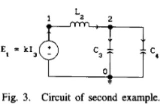
Fig. 3. Circuit of second example.

b) Analysis of the Network Connection Energy: The con- nection energy in branch 1 is

Wf =

Jd

I;U:dt b L 1 L 2 ( 1 1 ( 0 - )

+

1 2 ( o - ) ) In branch 2, 1 LlL2 2 L1+ L2 b W,C =

Jd

I T U i d t = .(I1(0-)

+

12(0-))12(0-). In branch 3, current and voltage are finite in

t

= 0. Therefore,

w,.

= 0.

The network connection energy is 3

(26)

wc

=

cw;

= L 1 L 2 ( I l ( o - )

+

I 2 ( 0 - ) ) ' . (29)

2 L 1 + L2 i=l

From (27) and (28), we obtain

U: = SLi(Il(O+) - I l ( O - ) ) = 6A4l U$ = SL2(Iz(O+) - 1 2 ( 0 - ) ) = 6A@2 = U:. That is to say, flux is conserved in the loop formed by both inductors: A41 = A& = A $ . Then,

1 1 2 W" = Wf

+

W,C = ZA4Il(O-)

+

-A$12(0-) 1 2 = - A 4 ( I i ( O - )

+

Ii(O+)) 1

+

p 4 ( ' 2 ( 0 + )

+

Iz(0-1) = -LJ1(0+)2 - -L111(0-)2

+

-L212(0+)2 - -LzI2(0-)2. 1 1 2 2 1 1 2 2

Thus, W" is equal to the increment of the energy stored in the magnetic field created by both inductors. From (26), we derive that this increment is always

5

0.

Example 2: Given the network of Fig. 3, let us suppose that

we interconnect its branches in

t

= 0. If capacitors C, and C,

have different initial voltages, a current impulse is produced in the loop formed by both capacitors. This current impulse is converted into a voltage impulse by the controlled voltage

(27)

~-

-6-

LlL2 ( I ~ ( ( ) - ) + 12(o-)). (28) source E l . Due to this voltage impulse, the flux of inductor

L Z is not conserved and 12(0+)

#

1 2 ( O - ) . L 1 + L2

892 IEEE TRANSACTIONS ON CIRCUITS AND SYSTEMS-I: FUNDAMENTAL THEORY AND APPLICATIONS, VOL. 40, NO. 12, DECEMBER 1993 a ) Time-Domain Analysis with the State Equation: From

Ohm's law and Kirchhoff s laws, we derive

0

- c3U3 (0- )

- c 4 U 4 (0 - )

After some row and column elementary transformations, we obtain the following state equation:

L

0

J

where the new variables are

c3U3 (O-)+C4 U4 (0-)

c3+ c 4

Iz(0-1

+

(&

-

&)

AQ3

[$]

= h(t)etd

[

The matrix A is obtained immediately from (30). From this

result, it is easily derived that AQ3 is equal to the charge increment in the capacitor C3 between the instants 0- and O+.

(22), we can derive that the network connection energy is b) Analysis of the Network Connection Energy: Applying

The total connection energy of both capacitors is

1 W,C

+

W,C = -AQ3(U3(0-) - u4(0-)) 2 1 2 - (u4(0+) - u4(0-))] 2 = -AQ3[(U3(O-)

+

u3(0+)) 1 - - -

1c3u3(o+)2

- 5C3u3(0-)' 1 1 2 2

+

-c4u4(0+)2 - -C4u4(0-)'

which is equal to the increment of the energy stored in the electric field created by both capacitors.

El

(7

C2

(b)

same circuit with an additional resistor.

Fig. 4. Networks of third example. (a) Circuit with a C E loop. (b) The

Example 3: Let us consider the network of Fig. 4(a). The switch S is open for

t

<

0 and closed for

t 2

0. El is a continuous function in ] - t, +m[. We are going to analyze the connection energy of this circuit.

The capacitor current is I$ = AQij. Then,

I; = A Q ~ = -I;

where AQ is the charge increment of the capacitor:

AQ = Cz(Ei(0) - uz(O-)). The connection energy for each branch is

Wf = --AQ 1 E i ( 0 ) W,C = -AQ 1 Uz(O-).

2 2

So the network connection energy is W" = -AQ(Uz(O-) 1 - El(()))

2

=

--C,(E1(0)

1 -

u2(o-))2.

2

Now, we are going to give a physical interpretation for the energy W" in this circuit. To make the example simpler, we suppose that El(t) is a constant function. Then, in this circuit,

-W" is equal to the limit of the energy consumed in the

resistor of the network of Fig. 4(b) when R3 + 0 in the interval [0,

t ]

for any t such that 0

<

t

<

+m: It is easy to

verify that the resistor current for

t 2

0 is

1 13(t) = -(El - UZ(O-))exp R3 Therefore, 1 R 3 I 3 ( t ) ' dt = (El - U 2 ( O - ) ) z L r e x p

(2)

d t R3 0

It is clear that the limit of this expression when R3 -+ 0 is

-W".

Given any value of R3, the above expression shows that the energy absorbed by the resistor R3 in [0, +m[ is -Wc

too. This result is similar to the interpretation given by Goknar [12], although Goknar's interpretation was stated only for L or

TOLSA AND SALICHS: ANALYSIS OF LINEAR NETWORKS 893

C circuits without sources. However, if

& ( t )

is not a constant function, the energy consumed by R3 in [0, +CO[ is generally different from -W“ (for example, if El(t) is sinusoidal, the energy consumed by R3 is +m). On the other hand, it can be checked that our first interpretation of -W“ as the limit of the energy consumed by R3 when R3 + 0 in the finite interval [0, t] can be extended to not constant functions E1

( t )

if El

( t )

is derivable enough.

Therefore, we think that our interpretation of -W“ is better than Goknar’s. It should be investigated if our hypothesis is true for any RLCM circuit. However, this is a difficult problem since it involves singular perturbations in singular systems.

APPENDIX

Given a pencil of square matrices

S

+

AT, we are going to explain an algorithm to calculate a unimodular matrix F ( A ) and an invertible matrix D such that (13) holds. The matrices

F ( A ) and D will be calculated using elementary row and column transformations. Our algorithm is purely algebraic, such as the algorithm given by Fettweis [9].

The concept of elementary row and column transformations of polynomial matrices can be found in [I 11. If these transfor- mations do not depend on A, they are said to be strict. If one matrix is obtained from another by elementary transformations, these matrices are equivalent. If all the transformations are strict, then they are strictly equivalent.

The concept of the row echelon of a matrix is introduced by Campbell [13]. He gives this definition: a rectangular m x n matrix A which has rank T is said to be in row echelon form

if A is of the form

c r x n

[

o ( m - r ) x n ]

where the elements c;j of C (= C,,,) satisfy the following conditions:

1) cij = 0 if i

>

j.

2) The first nonzero entry in each row of C is 1.

3) If cij = 1 is the first nonzero entry of the ith column, then the j t h column of C is the unit vector e; whose only nonzero entry is in the ith position. This column is said to be a “distinguished” column.

For example, the following matrix is in row echelon form: 1 3 0 - 2 0 4 0

[!!i

:%E].

It is easy to program an algorithm to obtain the row echelon matrix of any matrix by elementary row transformations. We have the following properties:

Any rectangular matrix B can always be row reduced to

row echelon form by elementary row operations. That is to say, there always exists an invertible matrix G such that GB = A, where A is in row echelon form. The rank of the matrix B equals the rank of its row ech- elon form A and is equal to the number of distinguished columns of A .

The algorithm to obtain (13) is shown in the following example. Let us consider the nonsingular polynomial matrix S

+

AT(1):

Through strict elementary row transformations in the polynomial matrix

S

+

AT, the matrix T is transformed in its row echelon form. The resulting matrix is

If the rank of T equals the dimensions of

S

+

AT(1), then we have finished, since the submatrix T,(;) must be equal to the identity matrix and the submatrices S ~ ~ ’ y S ~ ~ ) cannot exist.

By means of strict elementary row transformations in

S(l)

+

AT(1) we derive the row echelon form of the submatrix

Therefore, the pencil S(l)

+

XT(l)is transformed into

The rank of the submatrix

equals its number of rows, since det

(S

+

AT)

#

0. Thus, exchanging some columns in S2

+

AT2we obtain

1

Id22

J

(the columns of the submatrix Ida2are the distinguished ). If the submatrices of S ( 3 )

+

AT(3)

Si;)

+

AT,(:),

Si;)

+

AT;;)

do not exist (due to the fact that

S

+

ATis a unimodular matrix), then we have finished too.

Though (not strict) elementary row transformations, the pencil S ( 3 )

+

AT(3)is transformed into

: Id22

J

Due to the fact that

894 IEEE TRANSACTIONS ON CIRCUITS AND SYSTEMS-I: FUNDAMENTAL THEORY AND APPLICATIONS, VOL. 40, NO. 12, DECEMBER 1993 Now we return to point 1 of this algorithm, operating

in the submatrix Si;)

+

AT,(:), instead of the matrix S

+

AT.However, all the elementary transformations of points 1, 2, 3, and 4 must be done in the whole matrix ~ ( 4 )

+

~ ~ ( 4 1 , not only in

s!;)

+

AT,(:). These operations

will finish in point 1 or 3 after a finite number of loops, since in each loop the dimensions of submatrix Si;)

+

AT,(:) is strictly smaller than the dimension of S

+

AT. In fact, the number of loops must be I rank

(T)+l. At the end of this process we will obtain the matrix

-A+AId, :

...

[

M :I]’

If all of the same elementary row transformations of points 1-5 are made in the identity matrix, the resulting matrix is a unimodular matrix F(A). The only column transformations in points 1-5 are the column exchanges of point 3. Exchanging the same columns in the identity matrix, we derive an invertible matrix D’. If we define

Id, :

D = D I

. . . _ _ _ _ _ _ _ _ _ . . .

[ M i : b ]

REFERENCES

[l] N. Balabanian, T. A. Bickart, and S. Seshu, Electrical Nehoork Theory. New York: Wiley, 1969.

[2] L. 0. Chua and P. Lin, Computer Aided Analysis of Electronic Cir- cuits: Algorithms and Computational Techniques. Englewood Cliffs,

NJ: Prentice-Hall, 1975.

[3] A. Dervisoglu, “State equations and initial values in active RLC net- works,” IEEE Trans. Circuit Theory, vol. CT-18, pp. 544-547, Sept.

1971.

[4] Y. Murakami, “A method for the formulation and solution of circuits composed of switches and linear RLC elements,” IEEE Trans. Circuits

Syst., vol. CAS-34, pp. 496-509, May 1987.

[5] A. Opal and J. Vlach, “Consistent initial conditions of linear switched networks,” IEEE Trans. Circuits Syst., vol. 37, pp. 364-372, Mar. 1990. [6] L. Schwartz, TMorie des Distributions. Paris: Hermann, 1966. [7] -, Mitodos Matem‘ticospara las Ciencias Fisicas. Madrid: Selec-

ciones Cientificas, 1969.

[SI J. F. Colombeau, Elementary Introduction to New Generalized Func-

tions. Amsterdam: North-Holland, 1985.

[9] A. Fettwels, “On the algebraic derivation of state equations,” IEEE

Trans. Circuit Theory, vol. CT-16, pp. 171-175, May 1969.

[IO] G. C. Verghese, B. C. U v y , and T. Kailath, “A generalized state-space

for singular systems,” IEEE Trans. Automat. Contr., vol. AC-26, pp.

[ I l l F. R. Gantmacher, The Theory of Matrices ( 2 vol.). New York: Chelsea, 1977 (vol. 1). 1989 (vol. 2).

[I21 I. C. Goknar, “Conservation of energy at initial time for passive RLCM networks.” IEEE Trans. Circuit Theory, pp. 365-367, July 1972. [13] S. L. Campbell and C. D. Meyer, Generalized Inverses of Linear

Transformations. New York: Dover, 1991.

811-831, Aug. 1981.

Javier Tolsa, photograph and biography not available at the time of publi- cation.

(13) holds. Observe that D’ has been obtained through exchanges of columns in the identity matrix. Then, it is

x+

must be a subset of the original variables Y+in (12).

Seen that the state _{Miquel Salichs, photograph and biography not available at the time of}