Activated Sludge Process Design & Simulation of a Domestic Wastewater Influenced by Wine Production

MASTER FINAL PROJECT

MASTER OF ENVIRONMENTAL ENGINEERING

Activated Sludge Process Design &

Simulation of a Domestic Wastewater

Influenced by Wine Production

Author

Oriol Fàbregas Oller June 2019

Director/s

Dra. Maria del Mar Micó Department of Chemical Engineering and Analytical Chemistry. University of Barcelona

1 - 38 INDEX 1. Abstract ... 3 2. Nomenclature ... 4 3. Introduction ... 5 4. Goals ... 7 5. Methodology ... 7 6. Results ... 10

6.1.1 Influent Analysis and Worst-Case Scenario Determination ... 10

6.1.2 Other Influent Parameters ... 12

6.1.2.1 Nutrients Ratio ... 12

6.1.2.2 COD Fractioning ... 12

6.2 AS Design ... 14

6.2.1 Introduction in the Design ... 14

6.2.2 AS Design with ASM1 Model ... 15

6.3 Simulation Process ... 15

6.3.1 Worst-Case Scenario Simulation ... 15

6.3.2 Pseudo-Dynamic Simulation ... 18

6.3.2.1 Nutrient Stream Calculation (Urea and Orthophosphates) ... 19

6.3.2.2 Pseudo-Dynamic Simulation Final Results ... 22

7. Conclusions ... 24

8. Appendix ... 25

8.1 Nutrient Ratio ... 25

8.2 AS Process Design Calculations ... 27

8.2.1 SRT Calculation ... 27

8.2.2 COD in the Effluent ... 28

8.2.3 HRT and Volume of the Reactor ... 29

8.2.4 Food/Microorganisms Ratio ... 30

8.2.5 Recirculation and Purge ratio... 30

8.2.6 Sludge Production... 32

2 - 38

8.3 Dynamic Simulation ... 34 9. References ... 37

3 - 38

1. Abstract

Urban wastewater can have different characteristics depending on its origin and the industrial component. When focusing on wastewater influenced by wine industry, these characteristics are very significant for the design of a Wastewater Treatment Plant. This wastewater gathers a high quantity of organic matter during the harvest of the grapes season (vintage). In this study are evaluated and solved the main difficulties in the design of an Activated Sludge (AS) process from an urban WWTP in a winery region in Aragón, Spain.

After a research, it has been concluded that the main challenges for the water treatment of urban winery regions like this are the high flowrate and high organic matter load, especially in the shape of readily biodegradable organic matter (mainly organic acids, sugars and alcohols). Another difficulty found has been the lack of nutrients needed for the microorganisms to biologically treat the organic matter in this wastewater.

After the research has been done, the peaks of organic matter have been solved by designing the AS process with the influent parameters from the month of October as a worst-case scenario. Designing the plant to meet parameters in this scenario ensures that the system will overcome the increase of organic load provoked during vintage period. The AS process will also perform properly during the rest of the year.

Secondly, through the influent analysis, the nitrogen scarcity challenge has been analyzed. It has been concluded that the minimum BOD5 ratio of BOD5:TKN:TP = 100:5:1 has not been achieved during some parts of the year. Because of this, the minimum nitrogen and phosphorous ratio in the Activated Sludge process has been increased into BOD5:TKN:TP = 100:7:1.2 to calculate the ammonia and orthophosphates addition that is needed in every month of the year.

Then, a preliminary design of the AS process has been performed according the ASM1 model and using the worst-case scenario influent. This model can give an idea of the dimensions of the system, which is adjusted and checked later through simulation. However, this model requires a COD fractioning, and, in this case, it hugely varies from a standard one because the readily biodegradable COD fraction (like organic acids, sugars and alcohols) takes a high percentage. COD fractioning from Beck and collaborators work (2005 (1)_{) has been used as a reference, since it is also devoted to urban wastewater from} a winery region. This fractioning suits better because it lowers the recalcitrant fraction of the COD in the influent and increases the biodegradable one.

4 - 38

After the ASM1 calculation, the design volume of the aerobic reactor has been set at 248.8 m3 _{and its Solid Retention Time has been stablished at 5 days. The design inlet} flowrate has been 1.5 times higher than the flowrate of the worst-case scenario influent. In the last part of the report, LynxASM1 software has been used to perform the simulation of the AS system and it takes the ASM1 values obtained in the preliminary design. A worst-case scenario and a yearly simulation have been made to assure that the effluent meets the legislation standards of a WWTP with no nitrogen release limitations.

2. Nomenclature

- AS: Activated Sludge

- WWTP: Wastewater Treatment Plant - COD: Chemical Oxygen Demand - SI: Non-biodegradable soluble COD - Ss: Readily biodegradable COD - So: Dissolved oxygen

- SNO: Nitrate and nitrite nitrogen - SNH: Ammoniacal nitrogen

- SND: Biodegradable soluble organic nitrogen - XI: Non-biodegradable particulate COD - XS: Slowly biodegradable COD

- XBH: Active heterotrophic biomass - XBA: Active autotrophic biomass

- XP: Particulate products arising from biomass decay - XND: Particulate biodegradable organic nitrogen - TSS: Total Suspended Solids

- BOD: Biological Organic Demand - SRT: Solids Retention Time - HRT: Hydraulic Retention Time - CD,BOD5: BOD load in the inlet

- Ks: Half-saturation coefficient for heterotrophs - Kd: Heterotrophic decay rate

- µH: Heterotrophic specific growth rate

- µH,MÁX Heterotrophic maximum specific growth rate - ƟX: SRT

- ƟX,MIN: Minimum SRT

- SS,OUT: Readily biodegradable COD in the outlet of the AS - YH: Heterotrophic yield

5 - 38

- Q: AS inlet Flowrate - V: Reactor Volume

- XBH,R: Heterotrophic biomass in the settler - QW: AS Purge flowrate

- R: Recirculation flowrate factor - Qrs: AS recirculation flowrate - Qin: AS inlet flowrate

- YH,OBS:Observed Heterotrophic yield

- XBH,W : Heterotrophic Biomass in the recirculation - rso: Oxygen consumption rate

- V: Reactor Volume - OR: Oxygen Rate

3. Introduction

The project has started with the analysis and characterization of the wastewater to be treated. Yearly data of a real influent from Aragon Autonomous Region, Spain, has been provided.

The wastewater data comes from a domestic sewage in a small town located in a wine region of the Autonomous Community of Aragón, Spain. Wine production is one of the most robust industries in the world and every year is increasing its production. The global production of wine in 2013 was of 265 MhL which 68% came from Europe (2)_.

Wine production has always been known as a clean process. However, there is a great quantity of waste generated for every liter of wine produced. It has been estimated that for every 100 kg of grapes, 23.5 kg of residues (skins, seeds, lees, etc.) and 141 kg of wastewater are produced (most from cleaning the tanks and bottling facilities) (3)_. If focusing just in wastewater, 1 to 4 liters of wastewater are generated for every liter of wine produced and it varies depending on the working period of the wine cellar (racking, bottling or vintage) (4)_{. These are the main characteristics of raw winery wastewater:}

- Variable pH: Slightly acidic due to the accumulation of fermentation process waste. However, the mixture with the rest of the domestic wastewater sets the pH value in the inlet of the AS process near to 7 almost all year.

6 - 38

- High organic load: The major constituents of these effluents are organic acids (tartaric, lactic and acetic), sugars (glucose and fructose) and alcohols (ethanol and glycerol). Except of polyphenols, a great part of them are biodegradable (5)_. - Lack of nutrients: There can be found a low concentration of nitrogen and

phosphorus, which may cause an imbalance on the recommended ratios for biological treatment when this effluent is submitted to conventional treatment. - Seasonal: Wine production involves several steps that take place during all year. Each one of them leads to significant variations in volume, organic load and other parameters of the wastewater.

The main environmental impact of winery wastewater when is not properly treated is eutrophication (due to an excess of easily biodegradable organic content like sugars or alcohols, not to nutrient excess) which can lead the consumption of the dissolved oxygen in rivers or lakes. Other impacts of winery wastewater can be the alteration of physiochemical properties of groundwater, the inhibition effects on plant growth (due to high electrical conductivity), and the hazardous effects produced by small concentration of some phenolic compounds (6,7,8)_.

However, the wastewater data that is being analyzed doesn’t have a high percentage of raw wastewater because, as it was said before, it comes from a small town where it is mixed with urban wastewater. This mixture is done to lower the risk of receiving high organic loads in the WWTP.

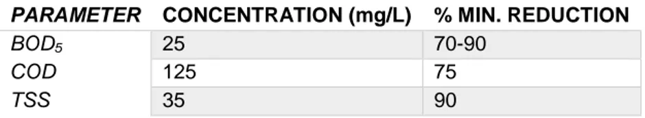
The treated water coming out from this WWTP will have to reach European Union legal requirements. These requirements are the ones marked in the “Council Directive 91/271/EEC concerning urban waste-water treatment” (9)_{, exactly the ones referring to} WWTP’s working with a secondary treatment. In Table 1 are shown the main parameters limits for these WWTP’s:

Table 1: Legal concentration requirements for wastewater disposal in the EU.

PARAMETER CONCENTRATION (mg/L) % MIN. REDUCTION

BOD5 25 70-90

COD 125 75

7 - 38

4. Goals

The general objective has been to determine the conditions of design and operation of a wastewater treatment based on an activated sludge system and that it guarantees a good quality of the effluent, despite the nutrient scarcity and the organic load and flow peaks caused by the wine industry activity in the area.

To achieve this objective, the following steps have been pursued and achieved: - Analysis of the annual influent data.

- Determination of worst-case scenario of operation.

- Preliminary calculation of the design according to the ASM1 model and based on the worst-case scenario.

- Simulation of the process according to the results of the ASM1 calculation until reaching the design and operation conditions that allow to obtain an effluent within the legal limitations.

- Verification, with a yearly simulation, that the limitations are also met throughout the year, maintaining the same design and operation conditions.

5. Methodology

The methodology of this report involves all the tools used to pre-design and simulate and Activated Sludge process. The key tools used from design and simulation have been the ASM1 Model and the LynxASM1 simulator, respectively.

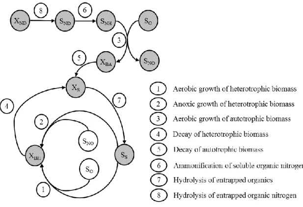
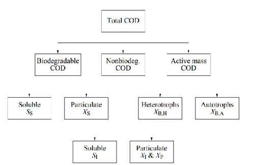
Activated Sludge Model No. 1 was created in 1983 by the International Association on Water Quality (IAWQ) and it facilitates the application of practical models or design and operations of biological wastewater treatment systems (10)_{. It easies the design because} it just involves 7 COD components, 7 Nitrogen components and 2 other components:

- SI: Non-biodegradable soluble COD - Ss: Readily biodegradable COD

- XI: Non-biodegradable particulate COD - XS: Slowly biodegradable COD

- XBH: Active heterotrophic biomass - XBA: Active autotrophic biomass

8 - 38

- XP: Particulate products arising from biomass decay - SNO: Nitrate and nitrite nitrogen

- SNH: Ammoniacal nitrogen

- SND: Biodegradable soluble organic nitrogen - XND: Particulate biodegradable organic nitrogen - SNI: Non-biodegradable soluble organic nitrogen - XNi: Particulate non-biodegradable organic nitrogen - XNP: Particulate nitrogen arising from biomass decay

- So: Dissolved oxygen - SALK: Alkalinity

This total of 16 variables are consumed or produced in a total of 8 dynamic processes in the biological reactors of activated sludge:

These 8 dynamic processes can be all simulated at the same time in a biological reactor using the LynxASM1 simulator. LynxASM1 is a free of charge simulation software designed by Aula Bioindicación Gonzalo Cuesta (ABGC) from IIAMA-UPV (Instituto de Ingeniería del Agua y Medio Ambiente de la Universitat Politècnica de València). This program allows to simulate AS processes in a very practical and easy way because it

9 - 38

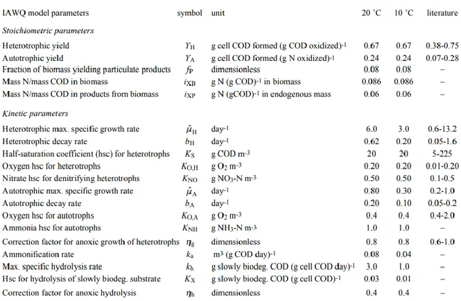
allows to change the inlet parameters of the previous 16 variables and the kinetic values of the following Table 2.

The kinetic parameters, as growth rate (Kd) or decay rate (µH) decrease their value as the temperature lowers because microorganisms are less active. During the design with ASM1 and simulation of this with LynxASM1, kinetics values at 10ºC have been used because the WWTP is located in a cold area and also because it is a worst-case scenario due to the low activity of the microorganisms.

10 - 38

6. Results

6.1.1 Influent Analysis and Worst-Case Scenario Determination

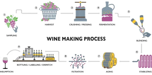
As said before, seasons have a significant importance in wine industry. Its production process can be summarized in the following six steps (As it is seen in Picture 1: Wine making process steps.): grape harvesting (1-2), crushing (3), fermentation (4), aging (7), filtration (8) and (9) bottling (11)_{. However, it can be simplified into vintage, aging and} bottling.

Vintage involves from harvesting to fermentation and it lasts from 2 to 6 weeks (in the North Hemisphere is set between August and October). This period produces the highest organic load and suspended solids concentration, it reduces the pH of the recipient water streams and it involves up to 50% of total water consumption. In the other hand, aging and bottling increase the pH of the recipient water streams due to the addition of NaOH into the tanks cleaning water processes.

Due to the high organic load the most difficult conditions to treat the wastewater are those related to the vintage season. Because of this, the average conditions of the consecutive Octobers from 2014 to 2016 have been selected as the design conditions for the simulation and as the worst-case scenario possible.

Table 3: Vintage wastewater parameters and their average values from 2014 to 2016

YEAR MONTH BOD5 COD pH TSS SNH SNO TKN TP FLOWRATE

2014 OCTOBER 1580.00 2782.33 6.41 557.46 16.40 1.41 37.25 5.97 122

2015 OCTOBER 1039.17 2534.39 6.35 408.72 12.51 3.30 39.35 7.74 159

2016 OCTOBER 1221.78 2460.88 6.06 356.24 6.33 4.20 20.60 4.43 151

11 - 38

YEAR MONTH BOD5 COD pH TSS SNH SNO TKN TP FLOWRATE

AVERAGE 1280.31 2592.53 6.27 440.80 11.75 2.97 32.40 6.04 144

(UNITS) mg/L mg/L mg/L mg/L mg/L mg/L mg/L m3_/day The most important parameters of the worst-case scenario have been the flowrate of 144 m3_{/day and the COD concentration of 2592.53 mg/L, which are key for the following} pre-design of the AS process.

As it can also be seen with TKN, SNH, COD and TSS values in Table 3, these parameters have been decreasing their concentration every year. This is because the wineries from the region have been increasing their wastewater treatment effectiveness in site in order to prevent fines and lawsuits from the local entities.

In the following Chart 1 are shown the legal required parameters from the 2016 to analyze the difference of organic load depending on the wine season:

As it is seen in both Table 3 and Chart 1, the organic load increases significantly in October compared with the non-vintage period (March to September). However, the flow is maintained during these months because the urban wastewater disposal from the town is stable during all year and it’s not influenced by the wine harvesting periods.

To sum up, if the AS process is designed with parameters from the worst-case scenario, it will assure that a quality effluent during the rest of the year.

0 20 40 60 80 100 120 140 160 180 0 500 1000 1500 2000 2500 FL o wr ate (m3/ h ) C o n ce n tr ati o n ( mg /L )

Flow COD BOD5 SS

12 - 38

6.1.2 Other Influent Parameters

6.1.2.1 Nutrients Ratio

A balanced nutrient ratio is crucial for microorganisms to grow and function effectively. These main nutrients are Nitrogen and Phosphorous and both are lacking when treating winery wastewater.

Because of that, there is the need to make a small calculation to see if this lack of nutrients is indeed real and to know how much of a nutrient addition would be needed. The maximum nutrient ratio for achieving microorganism’s growth is shown in Equation 1.

Nutrient scarcity is a common problem all year long, as we can see in the small calculation done in Appendix 8.1. BOD/TKN and BOD/TP ratios have been over the maximum in 13 and 20 of the 36 months from 2014 to 2016, respectively, being October the month where both nutrient lacks have been always present.

The worst-case scenario, which is the average of the months of October from 2014 to 2016, has had the following nutrient ratio.

Table 4: Nutrients analysis for worst-case scenario.

BOD5 (mg/L) TKN (mg/L) TP (mg/L) BOD5/TKN BOD5/TP

WORST-CASE 1280.31 32.40 6.04 39.52 211.86

As it was displayed before, the maximum ratio for Nitrogen and Phosphorous is 20 and 100, respectively, and in both cases those values are not reached in the worst-case scenario. The solution to this concern is to externally add urea (mainly ammonia) to increase TKN concentration and orthophosphates to increase TP concentration (these results are shown in Simulation Chapter 6.3).

6.1.2.2 COD Fractioning

A bibliographical research has been carried out to detail a suitable fractioning of COD contained in the influent. This fractioning is required to perform ASM1 calculation and also to do the mathematical simulation of the process.

𝐵𝑂𝐷5: 𝑇𝐾𝑁: 𝑇𝑃 = 100: 5: 1

𝐵𝑂𝐷5 𝑇𝐾𝑁 = 20

𝐵𝑂𝐷5 𝑇𝑃 = 100

13 - 38

In the ASM1 model it is estimated that in the inlet of the AS process there is zero concentration of biomass. Consequently, there are 4 parameters remaining in the COD fractioning:

- SI: Non-biodegradable soluble COD - Ss: Readily biodegradable COD

- XI: Non-biodegradable particulate COD - XS: Slowly biodegradable COD

For urban wastewater with the influence of winery industry, the COD fractioning used comes from Beck and collaborators work (2005 (1)_{) which characterizes a mixed urban} effluent from different spots from a winery region in Germany (Haut-Rhin).

Table 5: COD fractioning used in the design and simulation of the WWTP

BECK ET AL.

COD IWA (ASM1) Vintage period Non-vintage period

Ss 0.46 0.85 0.31

Si 0.04 0.012 0.15

Xs 0.47 0.094 0.5

Xi 0.03 0.05 0.04

As it is seen in Table 5, during vintage period, readily biodegradable COD (Ss) has a higher fraction due to the load of organic acids, sugars and alcohols. This fractioning is applied then for the worst-case scenario simulation and for October and November months in the dynamic simulation. In the other hand, ASM1 default domestic fractions are used in the dynamic simulation of non-vintage periods (10)_.

14 - 38

As COD fractioning is done, a preliminary calculation of the AS design has been developed by using the ASM1 model of the IWA (International Water Association) before making a simulation.

6.2 AS Design

6.2.1 Introduction in the Design

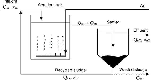
In its simpler version, the AS wastewater treatment process is based on an aerobic reactor followed by a settler where all the sludge created is separated from the cleared water. AS processes are optimal for the oxidation of high load of carbonaceous of biological matter. In Figure 3 there is a basic overlook of the process

Figure 3: Diagram of an activated sludge system process (13)

All nutrient removal operations have not been studied since the location of the WWTP is not a sensitive area according to BOE-A-2009-2347, referring to the Inspection report of the Management of the Tax for private use or special use of the local public domain (14)_. No restrictions are imposed in the nitrogen content of the WWTP effluent.

15 - 38

6.2.2 AS Design with ASM1 Model

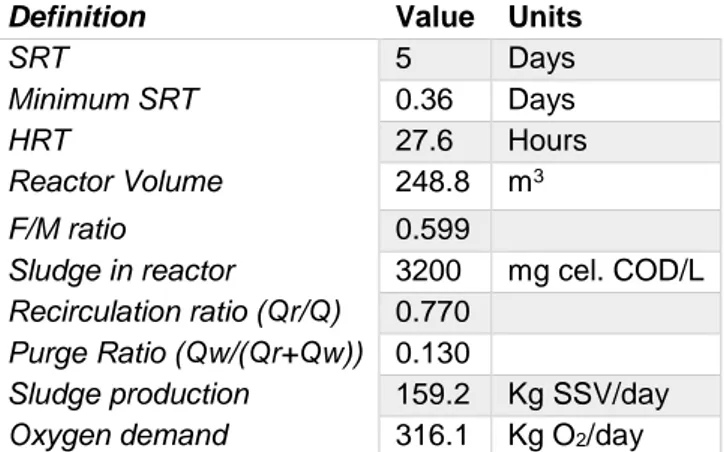
To obtain the preliminary design values of the AS, ASM1 model seen in Chapter “Methodology” has been used. Additional information regarding the Solids Retention Time (SRT) has been taken from the ATV-DVWK-A 131E standards (15)_{. After all the} calculations (shown in Appendix 8.2), Table 6 summarizes the main parameters obtained, which will be key for the simulation of the AS process. As it was said in in Chapter “Methodology”, all kinetic parameters from the ASM1 calculation are at 10ºC (10) _{and the} design flowrate is 1.5 times the worst-case scenario (216 m3_/day).

Table 6: ASM1 parameters obtained

Definition Value Units

SRT 5 Days

Minimum SRT 0.36 Days

HRT 27.6 Hours

Reactor Volume 248.8 m3

F/M ratio 0.599

Sludge in reactor 3200 mg cel. COD/L

Recirculation ratio (Qr/Q) 0.770

Purge Ratio (Qw/(Qr+Qw)) 0.130

Sludge production 159.2 Kg SSV/day

Oxygen demand 316.1 Kg O2/day

6.3 Simulation Process

6.3.1 Worst-Case Scenario Simulation

Once the initial calculations have been carried out, a worst-case scenario simulation with the software LynxASM1 has been executed. However, previously there has been the need to know which value of concentration of ammonia and ortophosphates is needed to reach the maximum BOD5/TKN and BOD5/TP ratio of 20 and 100, respectively.

The concentration needed to reach the maximum nutrient ratio of BOD5/TKN = 20 and BOD5/TP = 100 in the worst-case scenario is the next:

Table 7: Nutrients concentration required for the maximum the worst-case scenario.

Real Needed Added (Needed-Real)

TKN 32.40 64.02 31.62

16 - 38

By adding this new concentration in form of ammonia, the first simulation of the worst-case scenario has been carried (phosphorous is not considered in the ASM1 model). The following parameters have been added in the influent data:

Table 8: Worst-case scenario influent data with maximum nutrient ratio (Part 1)

Flowrate Ss Xs XBH XBA XP SO SNO SNH

Value 216 2206.65 246.7 0 0 0 0 2.97 43.37

Units m3_{/day mg COD/L mg COD/L mg COD/L mg COD/L mg COD/L mg O}

2/L mg NO3/L mg NH4/L

Table 9: Worst-case scenario influent data with maximum nutrient ratio (Part 2)

SND XND SALK SI XI

Value 9.11 11.54 100 31.11 129.63

Units mg N/L mg N/L mmol CO3-_{/L mg COD/L mg COD/L}

Then, by inserting the reactor volume, the recirculation ratio and the purge ratio into the software, the results of the first simulation have been the following:

As it can be seen in the simulation, there has not been a good organic matter removal since the concentration of readily biodegradable COD in the effluent (Ss), has been too high and it has not reached the compliance of the “Council Directive 91/271/EEC concerning urban waste-water treatment” (9)_{. The next step therefore has been to slightly} modify the nutrient maximum ratio to ensure that all the microorganisms have the enough nitrogen to grow.

Knowing that the maximum ratio of BOD5/TKN = 20 and BOD5/TP = 100 has not been enough to achieve a good quality effluent, the best option has been to lower the maximum ratio, so the ammonia concentration is higher during the simulation. The nutrient ratio for the AS process has been increased into the one in Equation 2:

17 - 38

Then, the new concentration of TKN and TP needed to reach the correct nutrient ratio in the worst-case scenario has increased into the one in Table 10 (in mg/L):

Table 10: Nutrients required for the worst-case scenario.

Real (mg/L) Needed (mg/L) Added (Needed-Real) (mg/L)

TKN 32.40 89.62 57.22

TP 6.04 15.36 9.32

Now, the inlet parameters have the same value as the ones in Table 8 y Table 9 except from the ammonia concentration (SNH), which has increased from 43.37 to 68.97 mg/L due to the change of the nutrient ratio. The results of the simulation with the new nutrient ratio are shown in the following Figure 5 and Table 11.

Table 11: Results of the simulation of the worst-case scenario.

Parameter Inlet Outlet Units % Reduction

Flowrate 216.00 191.12 m3_{/day -} Ss 2206.65 3.63 mg COD/L - Xs 246.70 0.14 mg COD/L - XBH 0.00 16.11 mg COD/L - XBA 0.00 0.03 mg COD/L - XP 0.00 3.93 mg COD/L - SO 0.00 2.00 mg O2/L - SNO 2.97 0.26 mg NO3/L - SNH 68.97 1.13 mg NH4/L - SND 9.11 0.70 mg N/L - XND 11.54 0.01 mg N/L - 𝐵𝑂𝐷5: 𝑇𝐾𝑁: 𝑇𝑃 = 100: 7: 1.2 𝐵𝑂𝐷5 𝑇𝐾𝑁 = 14.29 𝐵𝑂𝐷5 𝑇𝑃 = 83.33

Equation 2: Real nutrient ratio for the WWTP design.

18 - 38

Parameter Inlet Outlet Units % Reduction

SALK 100.00 95.38 mmol CO3-/L - SI 31.11 31.11 mg COD/L - XI 129.63 2.77 mg COD/L - COD 2614.09 57.73 mg COD/L 97.79 TSS 282.24 17.24 mg / L 93.89 BOD5 1280.31 2.36* Mg O2/L 99.82

* Outlet BOD Estimation = (Xs + Ss) / 1.6 (16)

As it can be seen in Table 11, the legal requirements of BOD, COD and Suspended Solids from Table 1 have been achieved in both concentration and in the percentage of minimum reduction. The main advantage is that if this design is suitable for the most strictive conditions, it also assures a good quality effluent during the rest of the year. However, a pseudo-dynamic simulation for all year has been done to ensure a good quality effluent every month of the year, and not just for the worst-case scenario of the month of October.

6.3.2 Pseudo-Dynamic Simulation

The inlet parameters used for this simulation have been the monthly averages from the 2014 to 2016, which are shown in Appendix 8.3. The AS design and operation conditions maintained were those obtained from the worst-case scenario simulation.

Twelve simulations (one for each month) have been performed. The parameters obtained from inside the reactor by the end of January simulation were transferred to the beginning of February simulation, and so on, in order to obtain a pseudo-dynamic simulation. No real dynamic simulation could be performed with this software since it does not provide the possibility to introduce variability in operating parameters such as the purge or the recirculation ratio. By the end of each month, the outlet parameters obtained were considered the averaged effluent values of the corresponding month. However, to assure that this pseudo-dynamic simulation has a final nutrient ratio of BOD5/TKN = 14.29 it has been key to know the TKN and TP necessary concentration in every month.

19 - 38

6.3.2.1 Nutrient Stream Calculation (Urea and Orthophosphates)

Urea

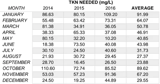
With the BOD5 monthly values of Appendix 8.1, the average of the TKN needed to get BOD5/TKN = 14.29in every month from 2014 to 2016 has been calculated with Equation 3 and is shown in Table 12.

Table 12: Monthly TKN values needed to achieve the sufficient nutrient ratio

TKN NEEDED (mg/L) MONTH 2014 2015 2016 AVERAGE JANUARY 86.63 80.15 109.20 91.99 FEBRUARY 55.48 63.42 73.31 64.07 MARCH 81.38 34.91 36.05 50.78 APRIL 38.33 65.33 37.08 46.91 MAY 80.15 32.20 10.20 40.85 JUNE 18.38 73.50 40.08 43.98 JULY 30.10 24.50 40.60 31.73 AUGUST 21.93 30.72 29.45 27.37 SEPTEMBER 28.70 16.45 26.50 23.88 OCTOBER 110.60 72.74 85.52 89.62 NOVEMBER 53.03 57.23 91.36 67.20 DECEMBER 24.50 19.25 44.89 29.55

With the TKN needed from the different months, the next step has been to know which of these months do already have this TKN needed in the influent or instead needs to be added externally. The following calculation to know the TKN to add in every month has been done:

Table 13: TKN to add for every month in the pseudo-dynamic simulation

MONTH Avrg. BOD5

(mg/L) Avrg. TKN Avrg.TKN Needed (mg/L) TKN to add (mg/L) JANUARY 1314.17 42.70 91.99 49.29 FEBRUARY 915.25 50.28 64.07 13.78 MARCH 725.42 31.29 50.78 19.49 APRIL 670.19 54.48 46.91 -7.57* MAY 583.56 47.42 40.85 -6.57* JUNE 628.33 41.05 43.98 2.93 JULY 453.33 52.47 31.73 -20.73* 𝑇𝐾𝑁 𝑡𝑜 𝑎𝑑𝑑 (𝑚𝑔 𝐿 ) = 𝑇𝐾𝑁 𝑁𝑒𝑒𝑑𝑒𝑑 ( 𝑚𝑔 𝐿 ) − 𝑇𝐾𝑁 ( 𝑚𝑔 𝐿 )

Equation 4: TKN to add equation

𝑇𝐾𝑁 𝑁𝑒𝑒𝑑𝑒𝑑 (𝑚𝑔

𝐿 ) = 𝐴𝑣𝑟𝑔 𝐵𝑂𝐷 ( 𝑚𝑔

𝐿 ) / 14.29

20 - 38

MONTH Avrg. BOD5

(mg/L) Avrg. TKN Avrg.TKN Needed (mg/L) TKN to add (mg/L) AUGUST 390.96 46.08 27.37 -18.72* SEPTEMBER 341.17 27.73 23.88 -3.85* OCTOBER 1280.31 32.40 89.62 57.22 NOVEMBER 960.05 31.92 67.20 35.28 DECEMBER 422.11 77.77 29.55 -48.22*

(*The ratio of BOD5:TKN:TP = 100:7:1.2 is already achieved so there is no need to add

nutrients externally.)

In 6 of 12 average months there is the necessity to add nitrogen to increase the TKN concentration. This is the reason why the nutrient addition stream of urea (mainly ammonia) has been calculated for every month simulation. The urea flowrate for every month has been achieved by knowing the design flowrate of the AS process (216000 L/day) and by knowing the TKN load this would mean. An example of the calculation is shown below:

The final values of the urea load are shown in the last column of Table 13:

Table 14: Urea load calculation every month

MONTH TKN Load (kg/day) Urea load (kg/day) JANUARY 10.6 23.146 FEBRUARY 2.977 6.473 MARCH 4.209 9.150 APRIL * * MAY * * JUNE 0.634 1.377 JULY * * AUGUST * * SEPTEMBER * * OCTOBER 12.360 26.869 NOVEMBER 7.621 16.567 DECEMBER * * 𝑇𝐾𝑁 𝑙𝑜𝑎𝑑 (𝑘𝑔 𝑑𝑎𝑦) = 𝑇𝐾𝑁 𝑡𝑜 𝑎𝑑𝑑 ( 𝑚𝑔 𝐿 ) · 1 𝑘𝑔 106_𝑚𝑔· 2,16 · 105 𝐿 1 𝑑𝑎𝑦 𝑈𝑟𝑒𝑎 𝑙𝑜𝑎𝑑 (𝑘𝑔 𝑑𝑎𝑦) = 𝑇𝐾𝑁 𝑙𝑜𝑎𝑑 ( 𝑘𝑔 𝑑𝑎𝑦) · 1 𝑘𝑔 𝑈𝑟𝑒𝑎 0,47 𝑘𝑔 𝑁

Equation 5: Calculation of the monthly TKN load

21 - 38

(*The minimum ratio of BOD5:TKN:TP = 100:7:1.2 is already achieved so there is no need

to add nutrients externally.)

Going back to the simulations, the urea addition produces the increase of the inlet SNH concentration during the pseudo-dynamic simulation into the next ones (SNH final):

Table 15: Final ammonia (SNH) inlet concentration in every month simulation

MONTH Avrg SNH (mg/L) SNH to add (mg/L) SNH final (mg/L)

JANUARY 25.850 49.290 75.140 FEBRUARY 26.717 13.780 40.497 MARCH 32.300 19.490 51.790 APRIL 33.683 * 33.683 MAY 33.133 * 33.133 JUNE 22.267 2.930 25.197 JULY 29.833 * 29.833 AUGUST 34.683 * 34.683 SEPTEMBER 17.633 * 17.633 OCTOBER 11.745 57.220 68.965 NOVEMBER 19.522 35.280 54.802 DECEMBER 29.667 * 29.667

(*The ratio of BOD5:TKN:TP = 100:7:1.2 is already achieved so there is no need to add

nutrients externally.)

Orthophosphates

In the other hand, the same calculations have been used to know the Orthophosphates flowrates: 𝑇𝑃 𝑙𝑜𝑎𝑑 (𝑘𝑔 𝑑𝑎𝑦) = 𝑇𝑃 𝑡𝑜 𝑎𝑑𝑑 ( 𝑚𝑔 𝐿 ) · 1 𝑘𝑔 106_𝑚𝑔· 2,16 · 105 𝐿 1 𝑑𝑎𝑦 𝑂𝑟𝑡𝑜𝑝ℎ𝑜𝑠𝑝ℎ𝑎𝑡𝑒𝑠 𝑙𝑜𝑎𝑑 (𝑘𝑔 𝑑𝑎𝑦) = 𝑇𝑃 𝑙𝑜𝑎𝑑 ( 𝑘𝑔 𝑑𝑎𝑦) · 1 𝑘𝑔 𝑂𝑟𝑡𝑜𝑝ℎ𝑜𝑠𝑝ℎ𝑎𝑡𝑒𝑠 0,33 𝑘𝑔 𝑃

Equation 9: Calculation of the monthly phosphorous load.

Equation 10: Ortophosphates monthly load calculation (17)

𝑇𝑃 𝑁𝑒𝑒𝑑𝑒𝑑 (𝑚𝑔 𝐿 ) = 𝐴𝑣𝑟𝑔 𝐵𝑂𝐷 ( 𝑚𝑔 𝐿 ) / 83.33 𝑇𝑃 𝑡𝑜 𝑎𝑑𝑑 (𝑚𝑔 𝐿 ) = 𝑇𝑃 𝑁𝑒𝑒𝑑𝑒𝑑 ( 𝑚𝑔 𝐿 ) − 𝑇𝑃 ( 𝑚𝑔 𝐿 )

Equation 7: TP Needed in every month

22 - 38

The final values of orthophosphates monthly loads are shown in the last column of Table 16. However, phosphorous is not considered in ASM1 model so there is not a change in the inlet parameters in the simulation like urea.

Table 16: Orthophosphates monthly load for every month.

MONTH Avrg. BOD5

(mg/L) Avg. P needed (mg/L) TP to add (mg/L) TP Load (kg/day) Ortophosphates Load (kg/day) JANUARY 1314.17 15.77 9.984 2.157 6.535 FEBRUARY 915.25 10.98 4.952 1.070 3.241 MARCH 725.42 8.71 3.550 0.767 2.324 APRIL 670.19 8.04 * * * MAY 583.56 7.00 0.046 0.010 0.030 JUNE 628.33 7.54 1.279 0.276 0.837 JULY 453.33 5.44 * * * AUGUST 390.96 4.69 * * * SEPTEMBER 341.17 4.09 * * * OCTOBER 1280.31 15.36 9.321 2.013 6.101 NOVEMBER 960.05 11.52 6.369 1.376 4.169 DECEMBER 422.11 5.07 * * *

(*The ratio of BOD5:TKN:TP = 100:7:1.2 is already achieved so there is no need to add nutrients externally.)

6.3.2.2 Pseudo-Dynamic Simulation Final Results

By changing the inlet SNH in every month (as represented in Table 15) and running all the twelve simulations, in the following Chart 2 are displayed the monthly outlet concentrations achieved from the legal required parameters (COD and TSS). All the rest of the parameters obtained in the outlet are shown in Appendix 8.3.

Chart 2: Outlet COD and TSS in the outlet of the dynamic simulation of the WWTP.

0 2 4 6 8 10 12 14 0 10 20 30 40 50 60 70 80

JAN FEB MAR APR MAY JUN JUL AUG SEP OCT NOV DEC

SS (m g/L) COD (m g/L) COD TSS

23 - 38

As it can be seen in Chart 2, the concentration of COD and TSS have never reached the maximum legal required values of 125 mg/L and 35 mg/L. each. Since the ASM1 model and simulation do not work with BOD5, it is not possible to know whether the legal limit of 25 mg/L has been exceeded in the tested period. However, as it is seen in the outlet concentration values in Appendix 8.3, the biodegradable fractions of the COD (Xs and Ss) have almost been eliminated. The remaining COD in the outlet stream comes from the non-biodegradable soluble fraction (Si) which is not involved with the concentration of BOD5 and cannot be removed from the wastewater by biological processes. This fraction cannot be extracted by settling and purging either because it is dissolved.

The main weakness from the dynamic simulation has been the excess of nitrates in the outlet stream of treated water related to the external dosing of nutrients, as it is seen in the following Table 17.

Table 17: Nitrates concentration in the outlet stream of the WWTP

As it is seen in Table 17, the SNO concentration exceeds 15 mg/L in January, March and December and exceeds 10 mg/L also in July and August. These two values of 10 mg/L and 15 mg/L of nitrates are key because these are the legal concentration limit of Nitrogen (which include TKN, nitrites and nitrates) by the “Council Directive 91/271/EEC concerning urban waste-water treatment”(9)_{. 15 mg/L of nitrogen is the limit from WWTP treating} water from 10,000 to 100,000 inhabitants and 10 mg/L of nitrogen is the one from WWTP for more than 100,000 inhabitants in sensitive regions.

According to what is explained in BOE-A-2009-2347, referring to the Inspection report of the Management of the Tax for private use or special use of the local public domain (14)_, the current WWTP is located in an area where no regulations on nitrogen concentration are applied. However, this nitrate excess could be prevented by implementing an automated control that regulates the amount of nutrients to add by detecting the COD that is entering the AS process at every moment.

JAN FEB MAR APR MAY JUN JUL AUG SEP OCT NOV DEC

24 - 38

7. Conclusions

Urban wastewater influenced by wine industry has chemical characteristics that widely vary depending on the harvest period that is occurring. Vintage period (set between August and October in the North Hemisphere and between February and April in the South Hemisphere) always produces the most difficult water to treat due to the important increase in the wastewater organic load. Because of this, the worst-case scenario of water treatment in this urban WWTP designed is in October, when there is an average inlet flowrate of 144 m3/day and COD concentration of 2592.53 mg/L. The organic load from the wine industry that is added to the urban wastewater is mainly easily biodegradable (in form of sugars, organic acids and alcohols). Consequently, the COD fractioning during vintage periods significantly differs in comparison with a standard urban wastewater. Readily and slowly biodegradable COD fractions (Ss and Xs) widely increase due to this load.

During high organic load months, a scarcity of biologically required nitrogen and phosphorous appears in the water to be treated. This should be solved by external addition of nutrients, which could be calculated with the starting minimum ratio of BOD5:TKN:TP=100:5:1.

The ASM1 model has allowed to obtain a pre-design of the AS system that could treat 216 m3_{/day of worst-case scenario wastewater effectively, by implementing an aerobic} reactor of 248,8 m3 _{in the system.}

With the results of the ASM1 pre-design and with the starting nutrient ratio, the worst-case scenario simulation of the system has been carried out but the minimum legal requirements for the outlet water have not been fulfilled. As a solution, the nutrient ratio has been raised into BOD5:TKN:TP=100:7:1.2 which successfully achieved the legal requirements by incrementing the TKN concentration.

The monthly flowrates of urea and orthophosphates have been obtained with the new optimal nutrient ratio. With this data it has been possible to perform a pseudo-dynamic simulation of an entire year in the AS process. It has effectively treated the water under the maximum legal concentrations of BOD5, COD and TSS for all twelve months.

25 - 38

8. Appendix

8.1 Nutrient Ratio

The following tables have been used to analyze in Chapter 6.1.2.1 the nutrients from the influent data given.

Table 18: 2016 Nutrient Analysis

Table 19: 2015 Nutrient Analysis

MONTH BOD5 TKN TP BOD5/TKN BOD5/TP

JANUARY 1145 46.0 5.14 24.92 222.76 FEBRUARY 906 50.3 9.45 18.01 95.87 MARCH 499 1.9 4.32 258.42 115.45 APRIL 933 63.2 7.39 14.77 126.30 MAY 460 60.2 9.07 7.65 50.72 JUNE 1050 46.6 7.06 22.53 148.73 JULY 350 43.4 2.89 8.06 121.11 AUGUST 439 55.4 7.47 7.93 58.74 SEPTEMBER 235 33.6 6.47 6.99 36.32 OCTOBER 1039 39.4 7.74 26.41 134.26 NOVEMBER 818 44.8 4.22 18.27 193.95 DECEMBER 275 37.5 4.26 7.33 64.55 MAXIMUM RATIO 20 100

Table 20: 2014 Nutrient Analysis

MONTH BOD5 TKN TP BOD5/TKN BOD5TP

JANUARY 1238 39.2 6.37 31.61 194.27

FEBRUARY 793 60.2 3.07 13.18 258.56

MARCH 1163 43.4 5.32 26.82 218.72

APRIL 548 68.9 16.50 7.95 33.18

MONTH BOD5 TKN TP BOD5/TKN BOD5/TP

JANUARY 1560 43.0 5.85 36.28 266.67 FEBRUARY 1047 40.4 5.58 25.92 187.68 MARCH 515 48.6 5.83 10.60 88.34 APRIL 530 31.4 4.70 16.90 112.71 MAY 146 34.3 3.44 4.25 42.34 JUNE 573 36.3 5.54 15.77 103.34 JULY 580 52.3 9.57 11.09 60.61 AUGUST 421 47.2 9.07 8.91 46.39 SEPTEMBER 379 24.9 5.27 15.20 71.82 OCTOBER 1222 20.6 4.43 59.31 276.11 NOVEMBER 1305 29.1 6.37 44.93 204.89 DICEMBER 641 138.0 23.40 4.65 27.41 MAXIMUM RATIO 20 100

26 - 38

MONTH BOD5 TKN TP BOD5/TKN BOD5TP

MAY 1145 47.8 8.36 23.95 136.96 JUNE 263 40.3 6.19 6.52 42.44 JULY 430 61.7 10.30 6.97 41.75 AUGUST 313 35.7 8.09 8.78 38.75 SEPTEMBER 410 24.7 6.69 16.60 61.29 OCTOBER 1580 37.3 5.97 42.42 264.88 NOVEMBER 758 22.0 4.87 34.49 155.54 DECEMBER 350 57.8 5.65 6.06 61.95 MAXIMUM RATIO 20 100

27 - 38

8.2 AS Process Design Calculations

The following pre-design parameters of the AS systems have been obtained with the ASM1 Model equations and with the influent values of the worst-case scenario from Table 3: Vintage wastewater parameters and their average values from 2014 to 2016

8.2.1 SRT Calculation

Solid Retention Time estimation has been done by picking the recommended one in the ATV-DVWK-A 131E standards. Previously, a calculation of the BOD load has been made to decide whether to use 5 or 4 days of SRT (as the Table 21 shows).

As it is seen in Table 21 the final SRT for the design of the AS without nitrification is 5 days. However, the minimum SRT has been calculated before to ensure that these 5 days of final SRT can be reached. Minimum SRT is obtained with the following equation from the ASM1 model:

Equation 12: Calculation of the minimum SRT (ASM1 Model)

𝐶𝑑, 𝐵𝑂𝐷5( 𝑘𝑔 𝑑𝑎𝑦) = 𝐷𝑎𝑖𝑙𝑦 𝐵𝑂𝐷 𝑙𝑜𝑎𝑑 = 1280.31 𝑚𝑔 𝐵𝑂𝐷5 𝐿 · 216,000 𝐿 𝑑𝑎𝑦· 1 𝑘𝑔 106 _𝑚𝑔 = 276.55𝑘𝑔 𝑑 𝜇𝐻,𝑚𝑎𝑥 · ( 𝑆𝑠 𝑆𝑠 + 𝐾𝑠) = 1 𝜃𝑥,𝑚𝑖𝑛 + 𝐾𝑑

Equation 11: BOD load calculation with the ATV Standards

28 - 38

The minimum SRT of 0,36 days confirms the design SRT of 5 days.

8.2.2 COD in the Effluent

A calculation of the theorical concentration of outlet COD has been performed to ensure that the chosen SRT is the correct to treat the water to a concentration lower than the legal limit (legal limit viewed in Table 1: Legal concentration requirements for wastewater disposal in the EU.). The equation used from the ASM1 model has been the following one:

If the obtained concentration of readily biodegradable COD (SS,OUT ) sums with the concentration of soluble non-biodegradable COD (Si) in the inlet* we have a

concentration of COD in the outlet of 31.11 mg COD/L. This concentration of COD in the outlet is lower in than the legal limit viewed in Table 1 of 125 mg COD/L, which means that the SRT used will be enough to treat the water.

- Ks (Half-saturation coefficient for heterotrophs at 10ºC) = 20 mg COD/L - Kd (Heterotrophic decay rate at 10ºC) = 0.2 day-1

- 𝜇𝐻,𝑚𝑎𝑥 (Heterotrophic maximum specific growth rate at 10ºC) = 3 day-1

- 𝑆_{𝑆,𝑂𝑈𝑇} (Readily biodegradable COD in the outlet) = mg COD/L - 𝜃𝑥 (SRT) = 5 days 𝑆𝑆,𝑂𝑈𝑇 = 20𝑚𝑔 𝐶𝑂𝐷 𝐿 (1 + 0,2 𝑑 −1_{· 5 𝑑)} 3 𝑑−1· 5 𝑑 − (1 − 0,2 𝑑−1· 5 𝑑)= 3.077 𝑔 𝐶𝑂𝐷 𝐿 =( 𝑚𝑔 𝐶𝑂𝐷 𝐿 )

Equation 13: Readily biodegradable COD (Ss) in the outlet calculation.

- Ks (Half-saturation coefficient for heterotrophs at 10ºC) = 20 mg COD/L - Kd (Heterotrophic decay rate at 10ºC) = 0.2 day-1

- 𝜇𝐻,𝑚á𝑥 (Heterotrophic max. specific growth rate at 10ºC) = 3 day-1

- 𝑆𝑠 (Readily biodegradable COD in the inlet) = 2203.65 mg/L =2203.65 mg COD/L - 𝜃𝑥,𝑚𝑖𝑛 = Minimum SRT (days)

29 - 38

*The concentration of soluble non-biodegradable COD (Si) is the same in the inlet and in the outlet because it can’t be oxidized by the biomass and cannot be settled and then removed in form of sludge.

8.2.3 HRT and Volume of the Reactor

With the ASM1 model, it is possible to know the Hidraulic Retention Time (HRT) of the reactor only if a value of heterotrophic biomass (XBH) is estimated. Because of this, a concentration of heterotrophic biomass of 3200 mg COD/L has been estimated in the aerobic reactor for the worst-case scenario. In addition, a concentration of heterotrophic biomass of 6400 mg COD/L has also been estimated in the settler (XBH,R).

The HRT of the reactor is calculated with the following equation

The volume of the reactor can be obtained by multiplying the HRT with the design flowrate of the WWTP: - Q (WWTP Flowrate) = 216 m3_{/d = 2166,000 L/day} - V (Reactor Volume) = m3 𝐻𝑅𝑇_{𝑟𝑒𝑎𝑐𝑡𝑜𝑟} = 𝑌_𝐻· 𝜃𝑥 𝑋_𝐵𝐻· 𝑆𝑠 (1 + 𝜃_𝑥 · 𝑘_𝑑)− 𝐾𝑠 𝜃_𝑥 · 𝜇_{𝐻,𝑚á𝑥}− (1 + 𝜃_𝑥· 𝑘_𝑑)

- Ks (Half-saturation coefficient for heterotrophs at 10ºC) = 20 mg COD/L - Kd (Heterotrophic decay rate at 10ºC) = 0.2 day-1

- 𝜇𝐻,𝑚𝑎𝑥 (Heterotrophic maximum specific growth rate at 10ºC) = 3 day-1

-

- 𝑌𝐻 (Heterotrophic yield) = 0.67 mg cell COD formed (mg COD oxidized)-1

- 𝑆𝑠 (Readily biodegradable COD in the inlet) = 2203.65 mg/L =2203.65 mg COD/L

- 𝐻𝑅𝑇𝑟𝑒𝑎𝑐𝑡𝑜𝑟 (Hidraulic Retention Time of the reactor) = days

- 𝑋𝐵𝐻 (Heterotrophic Biomass in the aerobic reactor) = 3200 mg COD/L 𝐻𝑅𝑇𝑟𝑒𝑎𝑐𝑡𝑜𝑟 = 1,15 𝑑𝑎𝑦𝑠 = 27,64 ℎ𝑜𝑢𝑟𝑠

𝑉 = 𝑄 · 𝐻𝑅𝑇𝑟𝑒𝑎𝑐𝑡𝑜𝑟 = 216,000 𝐿

𝑑𝑎𝑦· 1,15 𝑑𝑎𝑦𝑠 = 248803 𝐿 = 248.8 𝑚 3

30 - 38

8.2.4 Food/Microorganisms Ratio

The food to microorganism (F/M) ratio is one of the most important design parameters of activated sludge systems because a good balance between substrate consumption and biomass generation prevents the microorganisms to die or to suffer bulking or foaming in the biomass. The equation to get the value of F/M ratio is the following one:

The efficiency of an activated sludge process can be defined by its F/M ratio, and for conventional activate sludge systems cannot be over 1,4 in high organic wastewaters to prevent the growth of filamentous bacteria, which will not settle easily due to its long tails. (18)

8.2.5 Recirculation and Purge ratio

The recirculation and purge ratio have been calculated with the following Equation 16 from the biomass mass balance in the activated sludge system. The flowrate of settled water that is going to be purged from the recirculation has been obtained with the following equation: 𝐹 𝑀= 𝑄 · (𝑆_𝑆− 𝑆_{𝑆,𝑂𝑈𝑇}) 𝑉 · 𝑋_𝐵𝐻 𝐹 𝑀= 0.598

- 𝑋𝐵𝐻 (Heterotrophic Biomass in the aerobic reactor) = 3200 mg COD/L

- 𝑋𝐵𝐻,𝑊 (Heterotrophic Biomass in the recirculation) = 6400 mg COD/L

Equation 15: Food/Microorganisms ratio equation using the readily biodegradable COD

- 𝑋𝐵𝐻 (Heterotrophic Biomass in the aerobic reactor) = 3200 mg COD/L

- 𝑆𝑆,𝑂𝑈𝑇 (Readily biodegradable COD in the outlet) = 3.077 mg COD/L

- 𝑆_𝑠 (Readily biodegradable COD in the inlet) = 2203.65 mg/L =2203.65 mg COD/L - V (Reactor Volume) = 248,8 m3 _{= 248,800 L}

- Q (AS inlet Flowrate) = 216 m3_{/d = 2166,000 L/day}

Equation 16: Purge flowrate equation with the ASM1 mass balance.

𝑄𝑤 =

𝑋𝐵𝐻· 𝑉 𝑋𝐵𝐻,𝑊· 𝜃𝑥

31 - 38

As it was said in Appendix 8.2.3, the initial estimation of the concentration of heterotrophic biomass in the secondary settler is the double of the concentration in the aerobic reactor. Obviously, the concentration of heterotrophic biomass from the recirculation stream will be the same, as it comes out from the settler.

This 24.88 m3_{/day is the flowrate of water which is high concentrated in biomass and that} would flow out of the AS process.

The recirculation flowrate is obtained by multiplying the inlet flowrate with the following recirculation factor.

- XBH (Heterotrophic Biomass in the aerobic reactor) = 3200 mg COD/L

The final flowrate of settled water that returns to the influent is 166.239 m3_/day.

- V (Reactor Volume) = 248,8 m3 _{= 248,800 L}

-

- 𝑄𝑤 (AS purge Flowrate) = L/day

𝑄𝑤 = 24880.26 𝐿 𝑑𝑎𝑦= 24.88 𝑚3 𝑑𝑎𝑦 𝑄𝑟𝑠 = 𝑄 · 𝑅 = 216 𝑚3 𝑑𝑎𝑦· 0.7696 = 166.239 𝑚3 𝑑𝑎𝑦

- 𝑄_𝑟𝑠 (WWTP recirculation Flowrate) = m3_/day

- 𝑄 (AS inlet Flowrate) = m3_/day

Equation 17: Recirculation factor equation with the ASM1 biomass mass balance

- 𝑋𝐵𝐻,𝑅 (Heterotrophic Biomass in the settler) = 6400 mg COD/L

-

- 𝐻𝑅𝑇𝑟𝑒𝑎𝑐𝑡𝑜𝑟 (Hidraulic Retention Time of the reactor) = 1.15 days

32 - 38

8.2.6 Sludge Production

Sludge production (Px) is obtained by applying the kinetic reactions shown in the ASM1 Model. There is going to be more or less production depending on the observed heterotrophic yield. The observed heterotrophic yield is obtained with the following equation of kinetic parameters.

The observed heterotrophic yield is going to be lower than the theoretical one (set in 0,67 mg cellular COD/mg COD oxidized) due to the low weather temperature in the WWTP and due to the short SRT of 5 days.

The total sludge production per hour and liter is the following: 𝑌𝐻,𝑂𝐵𝑆 =

𝑌𝐻 (1 + 𝑘𝑑· 𝜃𝑥)

- Kd (Heterotrophic decay rate at 10ºC) = 0.2 day-1

-

- 𝑌_𝐻 (Heterotrophic yield) = 0.67 mg cellular COD formed (mg COD oxidized)-1

- 𝑌_{𝐻,𝑂𝐵𝑆} (Observed Heterotrophic yield) = mg cellular COD formed (mg COD oxidized)-1

- 𝑆𝑆,𝑂𝑈𝑇 (Readily biodegradable COD in the outlet) = 3,077 mg COD/L

- 𝑆_𝑠 (Readily biodegradable COD in the inlet) = 2203.65 mg/L = 2203.65 g COD/m3

- Q (WWTP inlet Flowrate) = 216 m3_{/d = 2166,000 L/day}

Equation 18: Observed heterotrophic yield equation with the ASM1 Model

Equation 19: Sludge production equation with the ASM1 Model

𝑃𝑥 = 𝑝𝑥· 𝑄 = 737,19 𝑚𝑔 𝐶𝑂𝐷 𝐿 · 216000 𝐿 𝑑𝑎𝑦· 1 𝑘𝑔 1 · 106 _𝑚𝑔= 159.23 𝑘𝑔 𝐶𝑂𝐷 𝑑𝑎𝑦 𝑌_{𝐻,𝑂𝐵𝑆} = 𝑌𝐻 (1 + 𝑘_𝑑· 𝜃_𝑥)= 0.335 𝑔 𝑐𝑒𝑙𝑙 𝐶𝑂𝐷 𝑓𝑜𝑟𝑚𝑒𝑑 𝑔 𝐶𝑂𝐷 𝑜𝑥𝑖𝑑𝑖𝑧𝑒𝑑

33 - 38

This value of sludge production is not used during the simulation of the AS. However, this is a very important factor if a rigorous design of the settler is done. It is also a key factor to design a posttreatment of the purged sludge like thickening or dewatering.

8.2.7 Oxygen Demand

The oxygen demand has been calculated by applying the oxygen mass balance in the ASM1 model. Its value is not also used in the simulation, but it is needed if the final design of the aerobic reactor in case it would be required.

When the oxygen consumption rate is obtained, it needs to be multiplied with the volume to know the oxygen rate the reactor needs to carry on the aerobic functions well.

𝑟𝑆𝑂 = 𝑑𝑆𝑂 𝑑𝑡 = ( 1 − 𝑌𝐻 𝑌𝐻 ) 𝜇𝑚𝑎𝑥 ,𝐻· 𝑆𝑆 𝐾𝑆+ 𝑆𝑆 · 𝑋𝐵𝐻+ 𝑘𝑑· 𝑋𝐵𝐻 𝑂𝑅 = 𝑟𝑠𝑜 · 𝑉 - V (Reactor Volume) = 248,8 m3 _{= 248,800 L}

- OR (Oxygen Rate) = mg/day

𝑂𝑅 = 𝑟_𝑠𝑜 · 𝑉 = 1270.45 𝑚𝑔 𝑂2 𝐿 · 𝑑𝑎𝑦· 248,000 𝐿 · 1 𝑘𝑔 1 · 106 _𝑚𝑔= 316,09 𝑘𝑔 𝑘𝑔 𝑂₂ 𝑑𝑎𝑦

Equation 20: Oxygen consumption rate with the ASM1 oxygen mass balance.

Equation 21: Oxygen required rate in the aerobic reactor.

- Ks (Half-saturation coefficient (hsc) for heterotrophs at 10ºC) = 20 mg COD/L - Kd (Heterotrophic decay rate at 10ºC) = 0.2 day-1

- 𝜇𝑚𝑎𝑥 ,𝐻 (Heterotrophic max. specific growth rate at 10ºC) = 3 day-1

- 𝑌_𝐻 (Heterotrophic yield) = 0.67 mg cell COD formed (mg COD oxidized)-1

- 𝑆_𝑠 (Readily biodegradable COD in the inlet) = 2203.65 mg/L =2203.65 mg COD/L - 𝑟_𝑆𝑂 =𝑑𝑆𝑂

34 - 38

8.3 Dynamic Simulation

These are the parameters and concentration values of the mixture of inlet water and nutrients. These concentrations and flowrates are the average of the given values from 2014 to 2016.

Table 22: Inlet stream concentrations and parameters from the dynamic simulation of the WWTP

INLET FLOWRATE (m3_/day) Si (mg/L) Ss (mg/L) So (mg/L) SNO (mg/L) SNH (mg/L) SND (mg/L) XI (mg/L) XS (mg/L) XBH (mg/L) XBA (mg/L) XP (mg/L) XND (mg/L) RECIRCULATION FLOWRATE (m3_/day) JAN 97.000 60.751 698.638 0.000 2.915 75.140 5.278 45.563 713.826 0.000 0.000 0.000 3.942 99.534 FEB 101.333 58.816 676.384 0.000 2.820 40.497 7.381 44.112 691.088 0.000 0.000 0.000 5.514 102.869 MAR 113.000 48.730 560.391 0.000 9.012 51.790 6.144 36.547 572.574 0.000 0.000 0.000 4.590 111.848 APR 99.000 38.007 437.076 0.000 1.257 33.683 6.515 28.505 446.577 0.000 0.000 0.000 4.866 101.073 MAY 107.667 41.316 475.133 0.000 0.927 33.133 4.474 30.987 485.462 0.000 0.000 0.000 3.342 107.743 JUN 119.333 43.379 498.859 0.000 1.348 25.197 5.883 32.534 509.704 0.000 0.000 0.000 4.395 116.722 JUL 111.000 27.102 311.676 0.000 1.160 29.833 7.089 20.327 318.451 0.000 0.000 0.000 5.295 110.309 AUG 131.333 24.269 279.096 0.000 0.930 34.683 3.571 18.202 285.163 0.000 0.000 0.000 2.667 125.958 SEP 120.500 27.037 310.922 0.000 0.570 15.700 2.850 20.278 317.681 0.000 0.000 0.000 2.129 117.620 OCT 144.000 31.110 2203.653 0.000 2.970 68.965 6.469 129.627 243.698 0.000 0.000 0.000 4.832 135.707 NOV 143.333 17.144 1214.377 0.000 5.685 54.802 5.302 71.434 134.296 0.000 0.000 0.000 3.961 135.193 DEC 114.000 32.802 377.228 0.000 1.853 29.667 15.065 24.602 385.428 0.000 0.000 0.000 11.254 112.618

35 - 38

These are the concentration values obtained inside the biological reactor after the simulation of every entire month indicated. Every monthly value obtained is used as the initial configuration for the following month. By doing this, a more realistic dynamic simulation is assured.

Table 23: Reactor parameters at the end of every monthly simulation.

Si (mg/L) Ss (mg/L) So (mg/L) SNO (mg/L) SNH (mg/L) SND (mg/L) XI (mg/L) XS (mg/L) XBH (mg/L) XBA (mg/L) XP (mg/L) XND (mg/L) JAN 60.751 3.313 2.000 21.079 0.942 0.676 103.714 12.103 894.014 11.834 263.167 0.715 FEB 58.816 3.436 2.000 0.712 0.950 0.697 103.661 12.442 897.808 3.449 260.463 0.744 MAR 48.730 3.339 2.000 17.877 0.980 0.698 93.292 11.210 821.101 8.877 232.461 0.669 APR 38.007 3.335 2.000 5.258 0.945 0.722 66.536 7.730 568.205 5.104 169.436 0.471 MAY 41.346 3.422 2.000 1.008 0.965 0.686 76.605 9.214 665.343 3.432 192.046 0.546 JUN 43.379 3.564 2.000 0.195 0.976 0.703 86.654 10.896 765.627 1.294 213.825 0.650 JUL 27.102 3.339 2.000 12.794 0.975 0.774 51.923 6.136 448.826 7.009 131.335 0.385 AUG 24.269 3.363 2.000 14.070 1.102 0.708 52.711 6.451 467.703 8.284 130.611 0.386 SEP 27.037 3.690 2.000 0.052 0.755 0.682 54.953 9.706 480.117 0.205 136.328 0.408 OCT 31.110 3.628 2.000 0.102 1.034 0.663 695.274 19.855 2210.821 1.758 579.956 1.616 NOV 17.144 3.387 2.000 6.539 1.037 0.680 217.548 10.508 1213.699 8.634 321.915 0.865 DEC 32.802 3.339 2.000 20.735 0.982 0.891 63.720 7.622 557.273 10.334 160.120 0.512

36 - 38

These are the outlet stream concentrations of the AS process.

Table 24: Outlet stream concentration values of the WWTP.

OUTLET FLOWRATE (m3_/day) Si (mg/L) Ss (mg/L) So (mg/L) SNO (mg/L) SNH (mg/L) SND (mg/L) XI (mg/L) XS (mg/L) XBH (mg/L) XBA (mg/L) XP (mg/L) XND (mg/L) COD TSS JAN 72.120 60.751 3.313 2.000 21.079 0.942 0.676 0.519 0.061 4.470 0.059 1.316 0.004 70.488 4.818 FEB 76.453 58.816 3.436 2.000 0.712 0.950 0.697 0.518 0.062 4.489 0.017 1.302 0.004 68.641 4.792 MAR 88.120 48.730 3.339 2.000 17.877 0.980 0.698 0.466 0.056 4.106 0.044 1.162 0.003 57.903 4.376 APR 74.120 38.007 3.335 2.000 5.258 0.945 0.722 0.333 0.039 2.841 0.026 0.847 0.002 45.427 3.064 MAY 82.790 41.346 3.422 2.000 1.008 0.965 0.686 0.383 0.046 3.327 0.017 0.960 0.003 49.501 3.550 JUN 94.453 43.379 3.564 2.000 0.195 0.976 0.703 0.433 0.054 3.828 0.006 1.069 0.003 52.334 4.044 JUL 86.120 27.102 3.339 2.000 12.794 0.975 0.774 0.260 0.031 2.244 0.035 0.657 0.002 33.667 2.420 AUG 106.453 24.269 3.363 2.000 14.070 1.102 0.708 0.264 0.032 2.339 0.041 0.653 0.002 30.961 2.497 SEP 95.620 27.037 3.690 2.000 0.052 0.755 0.682 0.275 0.035 2.401 0.001 0.682 0.002 34.119 2.544 OCT 119.120 31.110 3.628 2.000 0.102 1.034 0.663 1.976 0.099 11.054 0.009 2.900 0.008 50.776 12.029 NOV 118.453 17.144 3.387 2.000 6.539 1.037 0.680 1.088 0.053 6.068 0.043 1.610 0.004 29.392 6.646 DEC 89.120 32.802 3.339 2.000 20.735 0.982 0.891 0.319 0.038 2.786 0.052 0.801 0.003 40.136 2.997

37 - 38

9. References

1. C. Beck, G. Prades, A. Sadowski, Activated sludge wastewater treatment plants optimization to face pollution overloads during grape harvest periods, Water Sci. Technol. 51 (1) (2005) 81–88.

2. OIV—International Organisation of Vine and Wine Situation Report for The World Vitivinicultural Sector in 2013. (www.oiv.int)

3. G.A. Brito, J.M. Peixoto, J.M. Oliveira, C. Oliveira, R. Nogueira, A. Rodrigues, Brewery and winery wastewater treatment: Some focal points of design and operation—In Utilization of by-products and treatment of waste food industry, in: V. Oreopoulou, W. Russ (Eds.), Chapter 7, Springer, London, 2007, pp. 1–22 4. D. Bolzonella, F. Fatone, P. Pavan, F. Cecchi, Application of a membrane bioreactor

for winery wastewater treatment, Water Sci. Technol. 62 (2010) 2754–2759. 5. Chapman, J., Baker, P., Wills, S., 2001. Winery Wastewater Handbook: Production,

Impacts and Management. Winetitles, Adelaide, Australia.

6. X. Melamane, R. Tandlich, J. Burgess, Anaerobic digestion of fungally pre-treated wine distillery wastewater, Afr. J. Biotechnol. 6 (17) (2007) 1990–1993.

7. S. Mohana, B.K. Acharya, D. Madamwar, Distillery spent wash: treatment technologies and potential applications, J. Hazard. Mater. 163 (1) (2009) 12–25. 8. P.J. Strong, J.E. Burgess, Treatment methods for wine-related and distillery

wastewaters: a review, Biorem. J. 12 (2) (2008) 70–87.

9. Council Directive 91/271/EEC of 21 May 1991 concerning urban waste-water treatment. OJ L 135, 30.5.1991, p. 40–52

10. IWA taskgroup on mathematical modelling for design and operation of biological wastewater treatment (2000). Activated sludge models ASM1, ASM2, ASM2d and ASM3, Scientific and Technical Report 9.

11. Traversac, J.B., Rousset, S., Perrier-Cornet, P., 2011. Farm resources, transaction cost and forward integration in agriculture: evidence from French wine producers. Food Pol. 36, 839e847.

38 - 38

12. The relationship between BOD:N ratio and wastewater treatability in a nitrogen-fixing wastewater treatment system. Slade AH, Thorn GJ, Dennis MA. Water Sci Technol. 2011;63(4):627-32. doi: 10.2166/wst.2011.215.

13. Chai, Q & Bakke, Rune & Lie, Bernt. (2006). Object-oriented modeling and optimal control of a biological wastewater treatment process. 2006. 218-223.

14. Resolución de 28 de octubre de 2008, aprobada por la Comisión Mixta para las Relaciones con el Tribunal de Cuentas, en relación al Informe de fiscalización de la Gestión de la Tasa por utilización privada o aprovechamiento especial de dominio público local. Publicado en: «BOE» núm. 36, de 11 de febrero de 2009, páginas 14531 a 14616 (86 págs.)

15. ATV-DVWK Standard A 131E. Dimensioning of Single-Stage Activated Sludge Plants. – 2000

16. Applications of Activated Sludge Models edited by Damir Brdjanovic, S. C. F. Meijer, C. M. Lopez-Vazquez, C. M. Hooijmans, Mark C. M. van Loosdrecht 17. IV Jornada de Transferencia de Tecnología sobre Microbiología del Fango Activo.

Determinación de la fracción de Nutrientes por Respirometría en procesos de depuración biológica aerobia. Emilio Serrano - SURCIS, S.L.

18. Impact of food-to-microorganisms ratio on the stability of aerobic granular sludge treating high-strength organic wastewater - Rania Ahmed Hamza, Zhiya Sheng, Oliver Terna Iorhemen, Mohamed Sherif Zaghloul, Joo Hwa Tay - Department of Civil Engineering, University of Calgary, 2500 University Drive NW, Calgary, AB, T2N 1N4, Canada