Aspects of Brill-Noether geometry in moduli theory of algebraic and tropical curves

(1)

UNIVERSITÀ DEGLI STUDI “ROMA TRE”

FACOLTÀ DI SCIENZE MATEMATICHE FISICHE E NATURALI

Aspects of Brill-Noether geometry in

Moduli theory of Algebraic and

Tropical curves

Tesi di Dottorato in Matematica

di

Silvia Brannetti

(XXIII-Ciclo)

Relatore

Prof. Lucia Caporaso

(2)

Introduction

The Brill-Noether theory for smooth curves is the study of special line bundles, i.e. of the line bundles L on a curve C such that H1_{(C, L) 6= 0. By Riemann-Roch this means that}

the H0 _{cohomology or space of holomorphic sections is larger than expected, hence that}

the divisor corresponding to the line bundle moves in a larger linear system. This theory is a broad and classical area of algebraic geometry, which dates back to Riemann and his work on Abelian functions [R876]. However, the study has been deeply and extensively carried out by Brill and Noether in the XIX century ([BN873]). Through the years many aspects of the theory of special linear series have been investigated, so that each of them has inspired a separate research area. Among these areas, for instance, we recall the classical study of the Brill-Noether varieties

Wdr(C) = {L ∈ PicdC : h0(L) > r},

and their dimension. This study focused on the properties of linear series on a curve C, hence suggesting the possible projective models of C. The original motivation to study these varieties was to classify differences among curves. To this aim the structure of the Brill-Noether varieties becomes interesting only when we look at special linear series.

In this setting there are other aspects coming up, such as the projective normality of curves, which is the property for a canonically embedded curve of having a complete linear series cut by the hypersurfaces of the ambient space in any degree. We notice that the canonical bundle is special.

Moreover it is worth mentioning Abel maps (we will recall the definition later), which take values in the Brill-Noether varieties W0

d(X). If the degree is g − 1 we have that when

X is smooth the variety W0

g−1(X) is a divisor inside Picg−1X, the so called Theta divisor

of the Jacobian variety of X. From this point of view we can include the study of the Theta divisor in the Brill-Noether theory, and this naturally leads to approach the Torelli theorem (for details on all of these subjects see [ACGH]).

The Brill-Noether theory for smooth curves has been widely developed, but when we think of families of curves we have to consider singular curves as well. However, for singular curves not much is known yet. We point out some recent developments in the case of binary curves in [C5].

(5)

distin-guished classes of curves: singular and tropical curves. The study of singular curves and their properties is still very active and open: many of the classical theorems proved for smooth curves hold no longer for singular ones. We will work on curves with at most planar singularities. Of course the easiest to handle are nodal curves, and in particular stable curves, that allow us to work with their moduli.

Tropical geometry is a recent branch of mathematics which relates algebro-geometric objects to purely combinatorial ones in such a way that ideally one should be able to obtain results in algebraic geometry after studying their combinatorial tropical counterpart. A tropical curve C of genus g in the sense of [BMV09] is a marked graph Γ endowed with some extra data (see Definitions 2.2.1 and 2.2.3). Given their graph nature, we can inter-pret tropical curves as degenerations of smooth curves, but we can as well find a different and deeper relation between stable curves and tropical ones given by duality. Indeed a tropical curve is associated to a graph which can be thought of as the dual graph of a sta-ble curve (see subsection 2.5.3). So we can actually view singular and tropical curves as being part of the class of degenerate curves, i.e. curves arising as limits of smooth curves through a degenerating process.

The motivations for my work are, on the one hand, my interest in the Brill-Noether theory itself, since there is a lot of beautiful classical geometry involved. Moreover many proofs of general facts concerning moduli of curves have been obtained in history by look-ing at the properties of suitable degenerate curves, as slook-ingular and tropical curves are. Hence in this perspective I hope that my results can help interpret in an easier way clas-sical problems.

The problems

Chapter 1 is devoted to singular curves, and we tackle the following problems:

1. Given a smooth projective curve C of genus g and a natural number d ≥ 1, we can

consider the product Cd _{and define the Abel map of degree d}

αd C: Cd−→ PicdC, (p1, . . . , pd) 7→ OC( d X i=1 pi);

it is a regular map, and in degree 1 it is injective when g ≥ 1. In the smooth case the image Imαd

Cof the Abel map coincides with the Brill-Noether variety Wd0(C). Of course it

is interesting to approach the problem of extending Abel maps to singular curves in such a way that they have a geometric meaning.

If X is a singular curve we can still define Abel maps: we consider the decomposition of X in irreducible components, X = C1∪ . . . ∪ Cγ, and set ˙X := X \ Xsing, where Xsingis

the set of singular points of X, and ˙Ci = Ci∩ ˙X. Then, let d = (d1, . . . , dγ) be a multidegree

with di≥ 0 for any i, and set

˙

Xd_{:= ˙}_Cd1

(6)

˙

Xd _{is a smooth irreducible variety of dimension d = |d|, open and dense in X}d _{:= C}d1

1 × · · · × Cdγ γ . We set αd_X: ˙Xd_{−→ Pic}d_X, _(p 1, . . . , pd) 7→ OX( d X i=1 pi),

and we call it the Abel map of multidegree d; it is a regular map. Abel maps for integral curves have been studied by Altman and Kleiman in [AK80], and later on in [EGK00], [EGK02], [EK05]. We notice that the completion of Abel maps for integral curves was a major step to prove autoduality of the compactified Jacobian ([EGK02]). This is an important property connected with the study of the fibers of the Hitchin fibration for GL(n) ([AIK76], [N10]).

For reducible curves, the problem of completing the Abel maps is open with a few exceptions as we shall explain. As it is well known, the non separatedness of the Picard functor, together with combinatorial hurdles, make the case of reducible curves much more complex. The first step in this direction was taken by Caporaso and Esteves in [CE06], where they construct Abel maps of degree 1 for stable curves. However, they do not describe explicitly the closure of the image of the completion of the map. It is interesting to notice that they consider stable curves as limits of smooth ones, approaching this way the study of Abel maps for families of curves. In this setting, the completion of α1

X can be

viewed as a specialization to the singular fiber of the Abel maps of the smooth fibers. Further improvements have been achieved for Gorenstein curves by Caporaso, Coelho and Esteves in [CCE08] using torsion free sheaves, and by Coelho and Pacini in [Co07] and [CP09], where, respectively, they construct Abel maps of degree 2 for curves with two components and two nodes, and in any degree for curves of compact type. So in all other cases this problem remains open.

On the other hand the situation is better understood in case d = g − 1 in [C2]: if X is a nodal connected curve of genus g, denote by Ad(X) the closure of ImαdX inside PicdX. Let

Wd(X) := {L ∈ PicdX : h0(L) > 0};

in Theorem 3.1.2. the author proves that if d is a stable multidegree such that |d| = g − 1, then

Ad(X) = Wd(X),

and hence that the Brill-Noether variety Wd(X) is irreducible. Let PXg−1 be the

compact-ified Jacobian in degree g − 1; it has a polarization given by the Theta divisor Θ(X), and the pair (P_Xg−1, Θ(X)) is a semiabelic stable pair as in [A02]. It turns out that the varieties Ad(XS) = Wd(XS), where XS is a partial normalization of X at a set S of nodes, are the

sets which give a stratification of Θ(X) (see Theorem 4.2.6. in [C2]).

In the first section of Chapter 1 we generalize this stratification in lower degree and give a characterization of the closure of the image of the Abel map of multidegree d for some classes of nodal curves, inside the compactified Picard variety Pd

(7)

[C1]. We recall that in this construction every point of Pd

X corresponds to a pair ( bXS, cMS)

where bXS is the blow up of X at a set S of nodes of X, and cMS is a balanced line bundle

(see below) of multidegree d on bXSup to equivalence. So our question can be posed in the

following way: which points of Pd

X are limits of effective Weil divisors on X?

We will study the following cases: irreducible curves on the one hand, and two types of reducible curves, namely curves of compact type and binary curves. Curves of compact type have the advantage and the special property that the generalized Jacobian is com-pact. Binary curves are nodal curves made of two smooth rational components meeting at g + 1 points. They form a remarkable class of reducible curves since they present the basic problems as all reducible curves, yet simpler combinatorics. Indeed, they have been used in the past as test cases for results later generalized to all stable curves, see for instance [C5],[Br99].

In order to answer our question, let XS be a partial normalization of a nodal curve X

at a set S of nodes. We define the set W+

dS(XS) = {L ∈ Pic

dSX_S : h0(Z, L|_Z) > 0 for all subcurves Z ⊆ X_S},

and consider the union of the W+

d_S(XS) when S varies among the subsets of Xsingand dS

is the restriction to XS of a balanced multidegree bdSon the partial blow up bXS. Similarly

to [C2][Theorem 4.2.6], we define f Wd(X) := G ∅⊂S⊂Xsing bdS ∈B≥0d (XS )b W_d+ S(XS),

where B_d≥0( bXS) is the set of strictly balanced multidegrees bdS ≥ 0 on bXSsuch that |bdS| = d,

and d_S = bd_S|XS.

In paragraph 1.2.1 we study directly the closure inside Pd

X of Ad(X) for irreducible

curves, and we prove that Ad(X) = Wd(X) giving a description of it in terms of the

Brill-Noether varieties W0

d−δS(XS) where XS is the normalization of X at a set of nodes S, and

δS = ]S.

In paragraph 1.2.2 we turn our attention to reducible curves: we describe the struc-ture of the varieties Wd(X) for curves of compact type, which is quite natural, and in the

last part we develop the study of Ad(X) and its closure inside PXd for binary curves. We

characterize it in terms of the varieties WdS(XS). If X is a binary curve of genus g and

1 ≤ d ≤ g − 1, we prove that the closure inside Pd

X of the union of the varieties Ad(X) as d

varies among balanced multidegrees on X, is exactly fWd(X). In other words, we define

Ad(X) :=

[

d∈B≥0_d (X)

Ad(X) ⊂ PXd,

then the main theorem states that f

(8)

Finally we study the simpler case when d = 1 giving a characterization of the closure of the image of the Abel map for all the stable curves such that the set B≥01 (X) of strictly

balanced multidegrees d ≥ 0 is nonempty, i.e. the so called d-general curves.

2. Let C be a smooth curve of genus g over an algebraically closed field k. The canonical

bundle ωC induces an embedding of C in Pg−1 if and only if C is not hyperelliptic; we

indicate the power ω_C⊗nby ωn

Cfor any n ∈ N. One says that C is projectively normal if the

maps

H0_(Pg−1_{, O}

Pg−1(k)) → H0(C, ωk_C) (2)

are surjective for every k ≥ 1. In other words, C is projectively normal if and only if the hypersurfaces of degree k in Pg−1_{cut a complete linear series on C for any k. If k = 1 and}

the map (2) is surjective, we say that C is linearly normal, which means that the curve is embedded via a complete linear series. If ωCis ample, then an equivalent formulation

states that C is projectively normal if the maps SymkH0_{(C, ω}

C) → H0(C, ωkC) (3)

are surjective for every k ≥ 1, because the surjectivity of all these maps when ωCis ample

implies the very ampleness of ωC.

If C is a smooth, non-hyperelliptic curve, Castelnuovo and Noether proved that its canonical model is projectively normal (see [ACGH]). For curves, though, the problem becomes harder: in the case of integral curves, in [KM09] the authors generalize Castel-nuovo’s approach proving that linear normality is equivalent to projective normality. For reducible curves yet not much is known: properties of the canonical map for Goren-stein curves, i.e. the map induced by the dualizing sheaf, are investigated in [CFHR99], whereas in [F04] the author gives a sufficient condition for line bundles on non-reduced curves to be normally generated (see 1.4.9). The projective normality of reducible curves is studied in [S91]; more in general, since the problem of studying projective normality reduces to the study of multiplication maps, we refer to [B01] and [F04] for these items.

In the second section of chapter 1 we investigate the projective normality of reducible curves restricting the problem to suitable subcurves. The first step is to study the quadratic normality, i.e. the surjectivity of the maps in (2) for k = 2. Let X be a connected, reduced and Gorenstein projective curve of genus g with ωX very ample. Assume that X has

pla-nar singularities at the points lying on at least two irreducible components. Our main result about quadratic normality is the following theorem.

Theorem 1. Let X be a curve as above, and set X = A ∪ B with A, B connected subcurves

being smooth at D := A ∩ B. If A 6= ∅ and the map µωA,ωX|A: H

0_{(A, ω}

A) ⊗ H0(A, ωX|A) → H0(X, ωA⊗ ωX|A)

(9)

We also study certain multiplication maps in order to establish sufficient conditions that imply the surjectivity of the map in (3) for some k (k-normal generation) assuming to know the surjectivity for (k −1) (see Proposition 1.4.23). Moreover at the end of the section we carry out a proof of the projective normality for binary curves following the approach suggested by Castelnuovo-Noether in [ACGH], and see some applications of our results. This part is based on a joint work with Edoardo Ballico (see [BB10]).

3. In the third section of chapter 1 we study some properties of semistable curves that

are related to Brill-Noether theory: in subsection 1.3.1 we prove Martens’ theorem and Mumford’s theorem for irreducible nodal curves generalizing the approach described in [ACGH]. Then, in subsection 1.3.2 we turn our attention to the possible projective models of semistable k−gonal curves. A nodal curve is said to be k−gonal if it admits a regular smoothing such that the general fiber is a smooth curves having a g1

k(i.e. a pencil of degree

k).

We study nodal curves with two components (which are often called vine curves) in-vestigating about sufficient and necessary conditions in order for them to be k−gonal. In other words we list the properties that a vine curve must have in order to be k-gonal, and vice-versa. This study is carried out more extensively for trigonal curves, and the techniques we use refer to [Br99], [C2], [C6], [EM02] and to [HM82] for the specific use of admissible covers. We also introduce the concept of weakly k−gonal curves, defined as the curves possessing a g1

k, and in the case of weakly trigonal curves we investigate, as

Caporaso does for hyperelliptic curves in [C6], if they are trigonal. As one can expect the answer is negative.

Chapter 2 is devoted to tropical curves, and more in general to tropical moduli. The classical Torelli map tg : Mg → Ag is the modular map from the moduli space Mg of

smooth curves of genus g to the moduli space Agof principally polarized abelian varieties

of dimension g, sending a curve C into its Jacobian variety Jac(C), naturally endowed with the principal polarization given by the class of the theta divisor ΘC. The Torelli map

has been widely studied as it allows to relate the study of curves to the study of linear (although higher-dimensional) objects, i.e. abelian varieties. Among the many known results on the Torelli map tg, we mention: the injectivity of the map tg (proved by Torelli

in [T13]) and the many different solutions to the so-called Schottky problem, i.e. the problem of characterizing the image of tg(see the nice survey of Arbarello in the appendix

of [M99]).

The aim of this chapter is to define and study a tropical analogous of the Torelli map and is based on a joint work with Margarida Melo and Filippo Viviani (see [BMV09]). In the paper [MZ07], Mikhalkin and Zharkov study abstract tropical curves and tropical abelian varieties. They construct the Jacobian Jac(C) and observe that the naive gen-eralization of the Torelli theorem, namely that a curve C is determined by its Jacobian Jac(C), is false in this tropical setting. However, they speculate that this naive

(10)

general-ization should be replaced by the statement that the tropical Torelli map ttr

g : Mgtr → Atrg

has tropical degree one, once it has been properly defined!

In [CV1], Caporaso and Viviani determine when two tropical curves have the same Jacobians. They use this to prove that the tropical Torelli map is indeed of tropical degree one, assuming the existence of the moduli spaces Mtr

g and Atrg as well as the existence of

the tropical Torelli map ttr

g : Mgtr → Atrg, subject to some natural properties. Indeed, a

construction of the moduli spaces Mtr

g and Atrg for every g remained open so far, at least to

our knowledge. However, the moduli space of n-pointed rational tropical curves Mtr 0,nwas

constructed by different authors (see [SS2], [Mi4], [GKM09], [KM09]). The aim of chapter 2 is to define the moduli spaces Mtr

g and Atrg, the tropical Torelli map tg : Mgtr → Atrg and

to investigate an analogue of the Torelli theorem and of the Schottky problem.

With that in mind, we introduce slight generalizations in the definition of tropical curves and tropical principally polarized abelian varieties. A tropical curve C of genus g in the sense of [BMV09] is given by a marked graph (Γ, w, l) where (Γ, l) is a metric graph and w : V (Γ) → Z≥0 is a weight function defined on the set V (Γ) of vertices of Γ,

such that g = b1(Γ) + |w|, where |w| :=

P

v∈V (Γ)w(v) is the total weight of the graph, and

the marked graph (Γ, w) satisfies a stability condition (see Definitions 2.2.1 and 2.2.3). A (principally polarized) tropical abelian variety A of dimension g is a real torus Rg_{/Λ as}

before, together with a flat semi-metric coming from a positive semi-definite quadratic form Q with rational null-space (see Definition 2.3.1). To every tropical curve C = (Γ, w, l) of genus g, it is associated a tropical abelian variety of dimension g, called the Jacobian of C and denoted by Jac(C), which is given by the real torus (H1(Γ, R)⊕R|w|)/(H1(Γ, Z)⊕Z|w|),

together with the positive semi-definite quadratic form Q(Γ,l)which vanishes on R|w|and

is given on H1(Γ, R) by Q(Γ,l)(

P

e∈E(Γ)ne· e) =

P

e∈E(Γ)n2e· l(e). The advantage of such a

generalization in the definition of tropical curves and tropical abelian varieties is that the moduli spaces we will construct are closed under specializations (see subsection 2.2.1 for more details).

The construction of the moduli spaces of tropical curves and tropical abelian varieties is performed within the category of what we call stacky fans (see section 2.1.1). A stacky fan is, roughly speaking, a topological space given by a collection of quotients of rational polyhedral cones, called cells of the stacky fan, whose closures are glued together along their boundaries via integral linear maps (see definition 2.1.1).

The moduli space Mtr

g of tropical curves of genus g is a stacky fan with cells C(Γ, w) =

R|E(Γ|)>0 / Aut(Γ, w), where (Γ, w) varies among stable marked graphs of genus g, consisting

of all the tropical curves whose underlying marked graph is equal to (Γ, w) (see defini-tion 2.2.5). The closures of two cells C(Γ, w) and C(Γ0_{, w}0_{) are glued together along the}

faces that correspond to common specializations of (Γ, w) and (Γ0_{, w}0_{) (see Theorem 2.2.8).}

Therefore, in Mtr

g , the closure of a cell C(Γ, w) will be equal to a disjoint union of lower

dimensional cells C(Γ0_{, w}0_{) corresponding to different specializations of (Γ, w).}

We describe the maximal cells and the codimension one cells of Mtr

(11)

Mtr

g is pure dimensional and connected through codimension one (see Proposition 2.2.9).

Moreover the topology with which Mtr

g is endowed is shown in [C8] to be Hausdorff.

The moduli space Atr

g of tropical abelian varieties of dimension g is first constructed as

a topological space by forming the quotient Ωrt

g/ GLg(Z), where Ωrtg is the cone of positive

semi-definite quadratic forms in Rg_{with rational null space and the action of GL}

g(Z) is via

the usual arithmetic equivalence (see definition 2.3.5). In order to put a structure of stacky fan on Atr

g, one has to specify a GLg(Z)-admissible decomposition Σ of Ωrtg (see definition

2.3.6), i.e. a fan decomposition of Ωrt

g into (infinitely many) rational polyhedral cones that

are stable under the action of GLg(Z) and such that there are finitely many equivalence

classes of cones modulo GLg(Z). Given such a GLg(Z)-admissible decomposition Σ of Ωrtg,

we endow Atr

g with the structure of a stacky fan, denoted by Atr,Σg , in such a way that the

cells of Atr,Σ

g are exactly the GLg(Z)-equivalence classes of cones in Σ quotiented out by

their stabilizer subgroups (see Theorem 2.3.7).

Among all the known GLg(Z)-admissible decompositions of Ωrtg, one will play a special

role in this paper, namely the (second) Voronoi decomposition which we denote by V . The cones of V are formed by those elements Q ∈ Ωrt

g that have the same Dirichlet-Voronoi

polytope Vor(Q) (see definition 2.3.9). We denote the corresponding stacky fan by Atr,V

g (see

definition 2.3.11). We describe the maximal cells and the codimension one cells of Atr,V

g

and we prove that Atr,V

g is pure-dimensional and connected through codimension one (see

Proposition 2.3.12). Atr,V

g admits an important stacky subfan, denoted by Azong , formed by

all the cells of Atr,V

g whose associated Dirichlet-Voronoi polytope is a zonotope. We show

that GLg(Z)-equivalence classes of zonotopal Dirichlet-Voronoi polytopes (and hence the

cells of Azon

g ) are in bijection with simple matroids of rank at most g (see Theorem 2.3.16).

After having defined Mtr

g and Atr,Vg , we show that the tropical Torelli map

ttr

g : Mgtr→ Atr,Vg

C 7→ Jac(C), is a map of stacky fans (see Theorem 2.4.5).

We then prove a Schottky-type and a Torelli-type theorem for ttr

g. The Schottky-type

theorem says that ttr

g is a full map whose image is equal to the stacky subfan Agr,cogrg ⊂

Azon

g , whose cells correspond to cographic simple matroids of rank at most g (see Theorem

2.4.10). The Torelli-type theorem says that ttr

g is of degree one onto its image (see Theorem

2.4.15). Moreover, extending the results of Caporaso and Viviani [CV1] to our generalized tropical curves (i.e. admitting also weights), we determine when two tropical curves have the same Jacobian (see Theorem 2.4.14).

Finally, we define the stacky subfan Mtr,pl

g ⊂ Mgtr consisting of planar tropical curves

(see definition 2.5.7) and the stacky subfan Agr

g ⊂ Azong whose cells correspond to graphic

simple matroids of rank at most g (see definition 2.5.1). We show that Agr

g is also equal

to the closure inside Atr,V

g of the so-called principal cone σ0prin(see Proposition 2.5.4). We

prove that ttr

(12)

Agr,cogr

g := Acogrg ∩ Agrg (see Theorem 2.5.12).

As an application of our tropical results, we study a problem raised by Namikawa in [N80] concerning the extension tgof the (classical) Torelli map from the Deligne-Mumford

compactification Mg of Mg to the (second) Voronoi toroidal compactification Ag V

of Ag

(see subsection 2.5.3 for more details). More precisely, in Corollary 2.5.13, we provide a characterization of the stable curves whose dual graph is planar in terms of their im-age via the compactified Torelli map tg, thus answering affirmatively to [N80, Problem

(9.31)(i)]. The relation between our tropical moduli spaces Mtr

g (resp. Atr,Vg ) and the

com-pactified moduli spaces Mg(resp. Ag V

) is that there is a natural bijective correspondence between the cells of the former and the strata of the latter; moreover these bijections are compatible with the Torelli maps ttr

g and tg. This allows us to apply our results about ttrg

(13)

Chapter 1

Aspects of Brill-Noether theory

for singular curves

1.1 Notation

Let us recall some basic facts about the construction in [C1] that we will use in what follows. We work over an algebraically closed field k. Throughout the paper a curve will be a reduced projective variety of pure dimension 1 over k. Moreover, we will deal with nodal curves, although some statements are more general. Let then X be a nodal curve, and let Xν _{−→ X be its normalization; if X}ν ν _{= t}γ

i=1Ciν is the decomposition of Xν into

smooth components of genus gi for every i = 1, . . . , γ, then the arithmetic genus of X is

g =Pγ_i=1gi+δ−γ +1. If Z is a subcurve of X of genus gZand Zc= X \ Z, we will denote by

δZ = ]Z ∩Zcand if ωXis the dualizing sheaf of X, we set degZωX= deg ωX|Z = 2gZ−2+δZ.

A curve X of genus g ≥ 2 is said to be stable if it is connected and if every component E ∼= P1is such that δE ≥ 3, which is equivalent to saying that the curve has finite

auto-morphism group. By a quasistable curve we mean a connected curve X such that every subcurve E ∼= P1 _{has δ}

E ≥ 2 and the ones with δE = 2, i.e. the exceptional components,

don’t intersect. If S is a set of nodes of a stable curve X, throughout the paper we will denote by XS the normalization of X at the nodes in S, and by bXS the quasistable curve

obtained by “blowing up” X at S. In what follows we will often call bXS a partial blow up

of X. Obviously XS is the complement in bXS of all the exceptional components.

In [C1] Caporaso constructs a compactification Pd,g → Mg of the universal Picard

variety, such that the fiber over a smooth curve X of genus g ≥ 2 is its Picard variety PicdX, whereas if X is a stable curve in Mg, then the fiber over it is PXd, a connected and

projective scheme, which has a meaningful description in terms of line bundles on the partial blowups of X.

(14)

multide-gree of L by

d = (d1, . . . , dγ),

where, if X = Sγ_i=1Ci is the decomposition of X in irreducible components, we have di=

deg L|Ci and d = |d|. We say that d is balanced if for any connected subcurve Z of X we

have that d wZ 2g − 2− δZ 2 ≤ di≤ d wZ 2g − 2+ δZ 2 , (1.1)

where wZ= degZωX, and for any exceptional component E of X we have L|E = OE(1).

We say d is strictly balanced if strict inequalities hold in (1.1) for every Z X such that Z ∩ Zc _{6⊂ X}

exc, where Xexc is the subcurve of the exceptional components of X (see

[C7]). We will denote by Bd(X) the set of balanced multidegrees on X, and by Bd(X) its

subset of strictly balanced ones.

We are going to introduce the scheme Pd

X by looking at its stratification; so let X be a

stable curve of genus g ≥ 2, then, for any d, Pd

X is a connected, reduced scheme of pure

dimension g, such that

Pd X= a ∅⊂S⊂Xsing d∈Bd(XS )b P_Sd, (1.2)

where P_Sd ∼= PicdSX_S, X_S ⊂ bX_S as above, and d

S = d|XS. In particular, the points in

Pd

X are in one-to-one correspondence with equivalence classes of strictly balanced line

bundles. Any such class is determined by S and by M ∈ PicXS. Hence a point of PXd can

be denoted by [M, S], where if cMS is a class of line bundles in Bd( bXS), then M := cMS|XS,

and, by construction, when restricted to every exceptional component of bXS, cMS is equal

to O(1).

A node n of X is said to be separating if X \ {n} is not connected; we denote by Xsing

the set of nodes of X, and by Xsepthe subset of separating nodes.

If X is a nodal connected curve of genus g, we will denote by Ad(X) the closure of ImαdX

inside PicdX. Moreover we define the Brill-Noether variety: Wd(X) := {L ∈ PicdX : h0(L) > 0}.

Let νS : XS → X be the normalization of X at the nodes in S. It induces the pullback

map ν∗

S : PicdX → PicdXS; if M ∈ PicdXS, we denote by FM(X) the fiber of νS∗over M , and

by WM(X) the intersection FM(X) ∩ Wd(X).

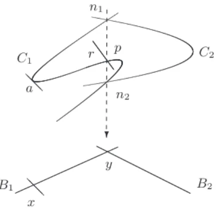
1.2 A compactification of the image of the Abel Map

Let αd_X be the Abel map of multidegree d of a stable curve X of genus g ≥ 2. We want to describe the closure of Imαd_X inside the compactified Jacobian Pd

X constructed in [C1]. We

(15)

1.2.1 Irreducible curves

Let X be an irreducible nodal curve of genus g and, for d ≥ 1, consider the Brill-Noether variety Wd(X). As a subvariety of PicdX, we are interested in studying its closure Wd(X)

in the compactified Picard Variety Pd

X, using the description given in [C1]. It will turn out

that Wd(X) is strongly related to the image of the Abel map, that we are going to define.

Let ˙X := X \ Xsing_{be the smooth locus of X; since X is irreducible, we have that ˙}_Xd _{is a}

smooth irreducible variety of dimension d, open and dense in Xd_{. Now, for d ≥ 1, let}

αd X : X˙d −→ PicdX (p1, . . . , pd) 7→ OX( d P i=1 pi); we call αd

Xthe Abel map of degree d. It is a regular map, and obviously αdX( ˙Xd) ⊂ Wd(X).

We denote by Ad(X) the closure of αdX( ˙Xd) in PicdX; of course Ad(X) ⊂ Wd(X). Let us

now introduce the following set f

Wd(X) := {[M, S] ∈ PXd s.t. h0( bXS, cMS) > 0},

where S ⊂ Xsing _{with δ}

S := ]S, bXS = XS∪ ∪δi=1S Ei is the blow up of X at the nodes of S,

and, as we introduced in the previous section, cMS is a class of line bundles in Bd( bXS) such

that its resctrictions to the components of bXS are

c

MS|XS =: M, McS|Ei = O(1) for any i = 1, . . . δS.

Let us observe that since h0_{( b}_X

S, cMS) = h0(XS, M ) (see [C2][Lemma 4.2.5]), we have:

f

Wd(X) = {[M, S] ∈ PXd s.t. h0(XS, M ) > 0},

which is in turn equivalent to: f Wd(X) ∼=

G

S⊂Xsing

Wd−δS(XS).

Theorem 1.2.1. Let X be an irreducible curve of genus g ≥ 1 with δ nodes. Then for any

d ≥ 1 we have:

(i) Ad(X) = Wd(X), hence Wd(X) is irreducible and dim Wd(X) = min{d, g},

(ii) Ad(X) = Wd(X) = fWd(X) ⊂ PXd.

Proof. We start by assuming that X has only one node n, and its normalization is ν : Xn→

X, with ν−1_{(n) = {p, q}. Let us consider the regular dominant map}

ρ : Wd(X) → Wd(Xn)

L 7→ ν∗_(L);

for any M ∈ Imρ we denote by WM(X) = ρ−1(M ), the fiber of ρ. We recall that WM(X) ⊂

(16)

cardinality of the fibers WM(X) is at least 0, so, since dim Wd(Xn) = d, it follows that

dim Wd(X) ≤ d; moreover Ad(X) is irreducible of dimension d, hence we have that Ad(X)

is an irreducible component of Wd(X). We want to prove that for any M ∈ Imρ, WM(X) ⊂

Ad(X), so that Ad(X) ⊂ Wd(X) ⊂ Ad(X) implies that Wd(X) = Ad(X) and Wd(X) =

Ad(X). We are now going to analyze all the possible cases.

(1) M ∈ Imρ with h0_(X

n, M ) = 1 and

h0_(X

n, M (−p)) = h0(Xn, M (−q)) = h0(Xn, M ) − 1.

Then by [C2, Lemma 2.2.3], WM(X) = {LM} with LM ∈ ImαdX.

n, M ) ≥ 2 and

h0(Xn, M (−p)) = h0(Xn, M (−q)) = h0(Xn, M ) − 1.

We are going to show that there exist two points in FM(X) ⊂ PXd which are contained

in Ad(X). Indeed,

FM(X) \ FM(X) = {[M (−p), n], [M (−q), n]}.

Let us take [M (−p), n]; by [C2, Lemmas 2.2.3, 2.2.4] there exists L ∈ Picd−1X such that ν∗_{(L) = M (−p) and L ∈ Imα}d−1

X . Let now pt∈ ˙X be a moving point specializing

to the node, i.e.such that pt −→ n. Of course L(pt→0 t) ∈ ImαdX, and L(pt) → [M (−p), n]

as t → 0. Then [M (−p), n] ∈ Ad(X). The same holds for [M (−q), n], so we have that

FM(X) \ FM(X) ⊂ Ad(X).

n, M ) = 1 and

h0(Xn, M (−p)) = h0(Xn, M (−q)) = h0(Xn, M ).

Again we want to prove that FM(X) \ FM(X) ⊂ Ad(X); so let M0 be a line bundle

on Xn not supported on either p or q such that M = M0(hp + kq); then M0 is as

in (1) and deg M0 _{= d}0 _{with d}0 _{= d − (h + k). Let us consider [M (−p), n] ∈ F} M(X),

then M (−p) = M0_(h0_{p + kq), where h}0 _{= h − 1. We choose a moving point p}

ton Xn

specializing to p as t goes to 0, and a moving point qton Xn such that qtspecializes

to q. Now fix t, and take the line bundle M00

t := M0(h0pt+ kqt) on Xn; by case (1),

there exists L00

t ∈ Imαd−1X such that ν∗(L00t) = Mt00. We consider now one moving point

pu∈ ˙X, such that ν∗(pu) on Xnspecializes to p when u → 0. As well as we saw in case

(2), L00

t(pu) ∈ ImαdX specializes to [Mt00, n] as u → 0. Hence [Mt00, n] ∈ Ad(X). Now let

t → 0: we see that, by construction, [M00

t, n] → [M (−p), n], hence [M (−p), n] ∈ Ad(X).

Using the same argument, we get that [M (−q), n] ∈ Ad(X) as well.

n, M ) ≥ 2 and either p or q as base point. Choose, say, p as

base point, i.e. h0_(X

(17)

M0 _{∈ Pic}d0

Xn, with M = M0(hp), d0 = d − h, and M0 not supported on either p or

q up to move the support away. We notice that M (−p) = M0_(h0_{p) with h}0 _{= h − 1,}

so, as before, we perform a double specialization to show that [M (−p), n] ∈ Ad(X).

Concerning [M (−q), n], we have that M (−q) = M0_{(hp − q) =: M}00_{(hp) for a suitable}

M00 _{∈ Pic}d0₋₁

Xn. Moreover, since p is a base point of M00(hp), h0(Xn, M00) ≥ 1. We

take again a moving point pton Xnspecializing to p, and a puon X such that ν∗(pu)

specializes to p on Xn. We fix t and denote Mt00 := M00(hpt), then by [C2, Lemmas

2.2.3,2.2.4] there exists L00

t contained in Imαd

0₋₁

X such that ν∗(L00t) = Mt00. We take

L00

t(pu); letting u → 0 we get that L00t(pu) → [Mt00, n] ∈ Ad(X). Now we let t → 0, and

obtain [M00

t, n] → [M (−q), n], whence [M (−q), n] ∈ Ad(X).

n, M ) ≥ 2 and h0(Xn, M (−p)) = h0(Xn, M (−q)) = h0(Xn, M ).

Then there exists M0_{∈ Pic}d0

Xn, with M = M0(hp + kq), d0= d − (h + k), and M0 not

supported on either p or q up to move the support away. As well as above, we consider [M (−p), n] and [M (−q), n] to show that they are contained in Ad(X). We proceed as

in case (3) performing a double specialization, and recalling that h0_(X

n, M0) ≥ 2 by

assumption.

Let U ⊂ Wd(Xn) be the following set:

U := {M ∈ Wd(Xn) s.t. h0(Xn, M ) = 1, h0(Xn, M (−p)) = h0(Xn, M (−q)) = 0};

this is of course an open set in Wd(Xn), and it contains all the line bundles M studied in

case (1). In particular for any M ∈ U , we have that Ad(X) intersects FM(X) in only one

point LM, where WM(X) = {LM}. In order to verify this assertion, by (1) we just have

to check that [M (−p), n] and [M (−q), n] are not contained in Ad(X), but this is obvious,

since h0_(X

n, M (−p)) = 0, hence on the blow up ˆXn of X at n, h0( ˆXn, \M (−p)) = 0. From

the study of all the possibilities above, from (2) to (5), we get that for any M ∈ Imρ which is not in U , Ad(X) contains at least two points of FM(X), but since the generic M has

](FM(X) ∩ Ad(X)) = 1, we have that for M ∈ Imρ \ U , the whole FM(X) must be contained

in Ad(X), hence for any M ∈ Imρ we have that WM(X) ⊂ Ad(X).

So we have shown that Wd(X) = Ad(X), with subsequent equality of their closures.

In order to show that Wd(X) = fWd(X), we argue like this: direction ⊂ is obvious, since

f

Wd(X) is a closed set in PdX containing Wd(X). On the other hand, the analysis made

above suggests that any [N, n] ∈ fWd(X) is also an element of Ad(X). Indeed if N has p

and/or q as base points, we argue as in (3),(4),(5); if otherwise N does not contain p nor q in its support, by (2) we get that there exists L(pt) ∈ ImαdX, such that L(pt) specializes to

[N, n] as t → 0.

If the number of nodes δ is ≥ 2, we proceed by induction on δ. Indeed, let X be a nodal irreducible curve having δ nodes. We blow up X at one node n, so that ˆXn is the blown up

curve, and Xnis the strict transform, and we have the normalization map ν : Xn→ X such

that ν−1_{(n) = {p, q}. So again we look at the dominant morphism ρ : W}

(18)

and we prove that the fibers WM(X) ⊂ Ad(X) for any M ∈ Imρ. As inductive hypothesis

we assume that Wd(Xn) = Ad(Xn) is irreducible of dimension d. This is the only point

where we used the smoothness of Xn in the previous case when δ = 1; hence reapplying

the argument above, which is based on [C2, Lemmas 2.2.3,2.2.4], we get the conclusions for every δ and for every d ≥ 1.

Remark 1.2.2. We observe that when d ≥ g, with g the genus of X, it doesn’t make sense

referring to Wd(X), since it is equal to PicdX. On the other hand, when d = 1 we have

that by [C2, Lemma 2.2.3], W1(X) = Imα1X = A1(X), and when d = g − 1 we get that the

Theta divisor is irreducible in Picg−1X.

Remark 1.2.3. From the equality Ad(X) = Wd(X) for any d, we deduce an important fact;

we use the previous notation, where X has δ nodes and Xnis the normalization at a node

n. Let L ∈ Wd(X) be such that M = ν∗L has WM(X) = FM(X). Then k∗ = WM(X), and

we can denote its elements in the following way:

WM(X) = {Lc, c ∈ k∗}.

By 1.2.1 we have that for any c ∈ k∗ _{there exists a family L}c

t ∈ ImαdX such that Lct → Lc.

In particular, we will have that Lc

t = ˜Lct(hpct+ kqtc) for suitable h, k, pct, qct ∈ ˙X such that

ν∗_(pc

t) specializes to p on Xn, ν∗(qct) specializes to q, and ˜Lct specializes to some effective

line bundle on X not supported on n. Hence we can assume ˜Lc

t = ˜Lcnot depending on t; so,

for any c ∈ k∗_{, we have ˜}_Lc_(hpc

t+ kqtc) → Lc. If ˜Lcis such that no other effective line bundle

is in its fiber, we have that ˜Lc_{= ˜}_{L, and ˜}_L(hpc

t+ kqtc) → Lc, so in this case the limit depends

only upon the choice of the moving points pc

t and qct. Equivalently, if c 6= c0 in k∗, there

exist moving points pc

t, qctand pc

0

t, qc

0

t such that ˜L(hpct+ kqtc) → Lcand ˜L(hpc

0 t + kqc 0 t) → Lc 0 .

1.2.2 Reducible curves

Very little is known about Abel maps of reducible curves, even if recently a lot of effort has been put into studying the class of stable curves, see for example [C2], [C5], [C6], [Co07],[CP09]. We are going to study the relation among the varieties Wd(X), Ad(X) and

their closures in Pd

X. Let X be a reducible curve with components C1, . . . , Cγ; for any

d = (d1, . . . , dγ) ∈ Zγ with |d| = d, we can consider the Brill-Noether variety Wd(X) that

we defined in the introduction of the paper. Obviously if di < 0 for every i = 1, . . . , γ, we

get that Wd(X) = ∅. On the other hand, if we assume d ≥ 0, i.e. di≥ 0 for every i, we can

define the Abel map of multidegree d. Set ˙X := X \ Xsing_{, and ˙}_C

i= Ci∩ ˙X; we define ˙ Xd:= ˙Cd1 1 × . . . × ˙Cγdγ⊂ Xd:= C1d1× . . . × Cγdγ, and αd_X : X˙d _−→ _Picd_X (p1, . . . , pd) 7→ OX( d P i=1pi).

(19)

As in the irreducible case, we denote by Ad(X) the closure of the set ImαdX ⊂ PicdX. We

are now going to introduce a set which will be crucial hereafter.

W_d+(X) := {L ∈ PicdX s.t. h0(Z, L|Z) > 0 for any subcurve Z ⊆ X}. (1.3)

This definition suggests the following

Lemma 1.2.4. Let d ≥ 0 be a multidegree on a reducible curve X. Then

Ad(X) ⊂ Wd+(X).

Proof. The proof is straightforward: the line bundles in Imαd_Xare of the form OX(

Pd i=1pi),

hence their restriction to any subcurve of X has nonzero sections. Then by upper semi-continuity of the dimension of the H0_{this is still true for their limits in A}

d(X).

We start by studying the simplest case, i.e. when X is a curve of compact type.

Curves of compact type

When X is a curve of compact type, for any multidegree d we have that Picd_{X is complete,}

hence so is Wd(X). However we are interested in the relation between Ad(X) and Wd(X).

We start by assuming that X has two smooth components C1, C2 meeting at one node n,

hence its normalization is the disconnected curve C1t C2−→ X,ν

with ν−1_{(n) = {p, q}. This induces the pullback map}

Pic(d1,d2)_X _{−→ Pic}ν∗ d1_C

1× Picd2C2,

which is an isomorphism, and given L ∈ Wd(X), we denote (L1, L2) := ν∗(L). We define

the sets: W_d+(X) := {L ∈ Wd(X) s.t. h0(C1, L1) > 0, h0(C2, L2) > 0}, W+− d (X) := {L ∈ Wd(X) s.t. h0(C1, L1) > 0, h0(C2, L2) = 0}, W_d−+(X) := {L ∈ Wd(X) s.t. h0(C1, L1) = 0, h0(C2, L2) > 0}; (1.4)

of course we have that Wd(X) = W_d+(X) t W_d+−(X) t W_d−+(X) set-theoretically.

Proposition 1.2.5. Let X be a curve of compact type of genus g with two smooth

com-ponents C1, C2 of genus resp. g1, g2. Let d ≥ 0 be a multidegree with |d| = d such that

1 ≤ d ≤ g − 1. We have:

(i) if d1≤ g1− 1 and d2≤ g2− 1, then Wd(X) is connected and has 3 irreducible

(20)

(ii) if d1≥ g1and d2≤ g2− 1 (up to swapping the indices), Wd(X) is connected and has 2

irreducible components.

Proof. In order to prove (i) we assume that d1 ≤ g1− 1 and d2 ≤ g2− 1. We consider the

pullback map

ν∗_{: Pic}d_X ∼=

−→ Picd1_C

1× Picd2C2

L 7→ (L1, L2);

then by [C2, 2.1.1] using that δ = 1, W+

d (X) = (ν∗)−1(Wd1(C1) × Wd2(C2)). (1.5) Now since C1, C2 are smooth curves, we have that Wdi(Ci) is irreducible of dimension di

for i = 1, 2. Then W_d+(X) is a closed irreducible set containing Ad(X). Since the fibers of ν∗

have cardinality one, dim W+

d (X) = d. By definition we know that Imα d

X= (ν∗)−1(ImαdC11× Imαd2

C2), hence dim Imα

d

X= d, then Ad(X) = Wd+(X) and they both have dimension d.

The other two components of Wd(X) are the following ones: consider L ∈ Wd+−(X); we

have that h0_(C

2, L2) = 0, and since L has nonzero sections, we have h0(C1, L1(−p)) > 0.

As in [C3] we define the set

Λp:= {L1∈ Picd1C1s.t. h0(C1, L1(−p)) > 0}, (1.6)

and consider the isomorphism

φp: Picd1−1C1 −→ Picd1C1

M 7→ M (p). (1.7)

It is easy to see that Λp = φp(Wd1−1(C1)), hence Λpis closed and irreducible of dimension d1− 1. Now consider the set

W+−d (X) := (ν∗)−1(Λp× Picd2C2);

it contains

W+−

d (X) = (ν∗)−1(Λp× (Picd2C2\ Wd2C2)) as an open set, and dim W+−_d (X) = d1+ g2− 1.

The last irreducible component of Wd(X) is the one containing the L’s such that h0(C1, L1) =

0 and h0_(C

2, L2) 6= 0. Arguing as before, we define the set Λq ⊂ Picd2C2, and the

isomor-phism φq : Picd2−1C2→ Picd2C2sending N ∈ Picd2−1C2to N (q). Hence Λq = φq(Wd2−1(C2)), and the set

W−+d (X) := (ν∗)−1(Picd1C1× Λq)

is the closure of W_d−+(X), with dim W−+d (X) = d2+ g1− 1. Hence we have that

Wd(X) = Ad(X) ∪ W

+−

d (X) ∪ W −+ d (X),

and their intersection is (ν∗₎−1_(Λ

p× Λq), having dimension d1− 1 + d2− 1 = d − 2. This

(21)

Part (ii) comes from part (i), once we have noticed that if d1 ≥ g1and d2≤ g2− 1, then

h0_(C

1, L1) > 0, so Wd−+(X) = ∅. Hence

Wd(X) = W_d+(X) ∪ W+−d (X),

and their intersection is (ν∗₎−1_(Λ

p), having dimension d1− 1. We notice that in this case

by (1.5), dim W_d+(X) = g1 + d2, which can be less than d. We prove that even in this

case it holds that W_d+(X) = Ad(X). Indeed, inclusion (⊃) is obvious, and concerning (⊂),

let us take a line bundle L ∈ W+

d (X). Then we look at its pullback M = ν∗(L). Let

M = (OC1(D1+ λp), OC2(D2+ µq)) for some suitable divisors D1and D2; we choose moving points pton C1∩ X and qton C2∩ X, specializing resp. to p and q. We consider on C1t C2

the line bundle:

Mt:= (OC1(D1+ λpt), OC2(D2+ µqt)),

and push it down to X, getting the (unique) line bundle Lt∈ Imαd_Xsuch that ν∗(Lt) = Mt.

Then if we let t tend to 0, we get that Ltspecializes to L, and hence that L ∈ Ad(X). So we

conclude that W_d+(X) = Ad(X). It follows that dim Wd(X) = max{g1+ d2, d1+ g2− 1}. If

vice-versa d2≥ g2and d1≤ g1− 1, we have that W_d+−(X) = ∅, Wd(X) = Ad(X) ∪ W−+d (X),

Ad(X) ∩ W −+

d (X) = (ν∗)−1(Λq), and dim Wd(X) = max{d1+ g2, d2+ g1− 1}.

Remark 1.2.6. We just observe that the case d = g −1 is carried out in [C2], but we obtain

it as a by-product in 1.2.5(ii); since there are no strictly balanced multidegrees summing to g − 1 on a curve of compact type, we get that Wd(X) is not irreducible.

In the sequel we will try to generalize our study to any curve of compact type, so take X as the union of irreducible smooth curves C1, . . . , Cγ, with gi the genus of Ci and g the

genus of X. Notice that since X is of compact type, we have that ](Ci∩ Cj) = 1 for i 6= j,

and this implies that the total number of nodes δ ≤ γ − 1; we denote by nijthe intersection

point Ci∩ Cj. Let d ≥ 0 be a multidegree on X, with |d| = d, 1 ≤ d ≤ g − 1. Let

ν :

γ

G

i=1

Ci→ X

be the total normalization map, ν∗_{the pullback as before, and denote by (L}

1, . . . , Lγ) the

pullback to Fγ

i=1

Ci of any L ∈ PicdX. If nij is a node, its branches on Ci, Cj will be called

respectively pi

j, pji, distinguishing the curve they belong to by the position of indices.

Lemma 1.2.7. Let X be a connected curve of compact type as above and d ≥ 0. Then

W+

d (X) = Ad(X), is a (closed) irreducible component of Wd(X).

Proof. The proof is straightforward: we see that, as we pointed out in the case γ = 2, W_d+(X) = (ν∗)−1(Wd1C1× · · · × WdγCγ), (1.8)

indeed X has a number of nodes δ = γ − 1, so we apply [C2, 2.1.1] and obtain the equality. Since Ci is smooth for every i, by (1.8) Wd+(X) turns out to be a closed irreducible set of

(22)

dimension d1+ · · · + dγ = d, and it contains Ad(X). To see the inverse inclusion we argue

as in 1.2.5(ii), proving that for any L ∈ W_d+(X) there exists Lt∈ ImαdXsuch that, if we let

t tend to 0, we get that Ltspecializes to L. So we have Wd+(X) = Ad(X) as we wanted.

What we are going to do now is to study the remaining irreducible components of Wd(X). To do this we need to introduce some notation: let δi= ](Ci∩X \ Ci) for i = 1, . . . , γ,

and let I be a 1 × γ vector where the j-th component is Ij = + or Ij = −. Then we can

define the set:

ª . Notice that if Ij= + for every j, i.e. I = (+, . . . , +), we get Wd+(X). Let us fix some vector

I 6= (+, . . . , +); set

I+:= {j ∈ {1, . . . , γ}, Ij= +},

and

I− _{:= {h ∈ {1, . . . , γ}, I}

h= −}.

We denote by pj_h the branch on Cj of the point of intersection Cj ∩ Ch, for j ∈ I+, and

some h ∈ I−_{, if it exists. Moreover, we fix j ∈ I}+ _{and consider the disconnected curve}

X \ Cj = X1jt · · · t Xkjj. We observe that Cj has only one point of intersection with each

X_lj, for l = 1, . . . , kj. We denote the branches of this point on Cjand Xjlresp. by pjl and plj.

If (L1, . . . , Lγ) are the restrictions of a line bundle L on X to each irreducible component

of X, we denote by L_Xl

j the restriction of L to the connected component X

l j. Set: Lj:= n l ∈ {1, . . . , kj}, h0(LXl j) = 0 o , and let Λj:= {Lj∈ Wdj(Cj), h 0_(L j(− X l∈Lj pj_l)) > 0}. Now, still for j ∈ I+_{, consider the set:}

e Σj :=  Y h∈I− (Picdh_C h\ Wdh(Ch)) × Λj× Y l∈I+_,l6=j Wdl(Cl)   ⊂ γ Y i=1 Picdi_C i. (1.9)

and denote by Σjthe set obtained from eΣjby reordering the factors in such a way that the

final order in Σj corresponds to the order of the components of I, so for example, Λj will

be the factor in the position of j in I. We will denote by ΣI =

[

j∈I+

Σj. (1.10)

We observe that Λjis irreducible (see 1.2.5), and its dimension depends on the cardinality

λj of Lj. Indeed dim(Λj) = dj− λj and 0 ≤ λj ≤ kj. It follows that Σj is irreducible for

(23)

Lemma 1.2.8. We have that (ν∗₎−1_(Σ

I) = W_dI(X).

Proof. Inclusion (⊂) is easy by definition of ΣI, since an element of (ν∗)−1(ΣI) must have

at least a nonzero section. On the other hand, given a line bundle L ∈ W_dI(X), we want to prove that ν∗_{(L) = (L}

1, . . . , Lγ) belongs to ΣI. If for every i ∈ I+, h0(LXl

i) 6= 0 for every

l = 1, . . . , ki, then Li= ∅ and Λi= Wdi(Ci) for every i, hence in this case

Σ = Y h∈I− (Picdh_C h\ Wdh(Ch)) × Y l∈I+ Wdl(Cl)

up to reordering the factors in the left hand side, and therefore ν∗_{(L) ∈ Σ. Now, assume}

that there exists i ∈ I+ _{such that L}

i 6= ∅. Without loss of generality we can assume

that |Li| = 1. Then in order to glue the sections and get a line bundle on X, it must be

h0_(L

i(−pil)) > 0, hence Li∈ Λi, and therefore

(L1, . . . , Lγ) ∈ Σj ⊂ ΣI.

Even if we can’t say precisely which is the dimension of the components of W_dI(X), we can count how many they are. By (1.10) we see that for any fixed I, the number of irreducible components of W_dI(X) is |I+_{|. Hence we can say that the number of irreducible}

components of Wd(X) is N :=  1 + X I6=(+,...,+) |I+_|   . (1.11)

Remark 1.2.9. We notice that depending on d, some I’s won’t appear in (1.11); indeed, if

there exists some k ∈ {1, . . . , γ} such that dk≥ gk, then the component Ikof I must be +, so

we will have a small number of I’s, and hence a small number of irreducible components in Wd(X). Moreover, if dk ≥ gk for every k, we get that the only irreducible component of

Wd(X) is Wd+(X).

Binary curves

A binary curve of genus g is a nodal curve made of two smooth rational components inter-secting at g + 1 points. We are going to recall some properties that we will use throughout this paragraph. If X is a binary curve of genus g ≥ −1, a multidegree d = (d1, d2) such

that |d| = d, is balanced on X if

m(d, g) := d − g − 1

2 ≤ di≤

d + g + 1

2 =: M (d, g) (1.12)

We say that d is strictly balanced if strict inequality holds. If bXS is a quasistable curve

obtained from a binary curve X by blowing up the nodes in S, then we call E1, . . . , E]S the

exceptional components, so that if XS is the partial normalization of X at the nodes in S,

(24)

Definition 1.2.10. A multidegree bd = (d1, . . . , d2+]S) on bXS with |bd| = d, is balanced if the

following hold:

(1) di= 1 for any i = 3, . . . , ]S, i.e. bd|Ei = 1, ∀i.

(2) bd|XS is balanced on XS.

b

d is strictly balanced if its restriction to XS is strictly balanced on XS.

Remark 1.2.11. Let X be a binary curve of genus g, and let Xn be the normalization of

X at the node n, such that ν : Xn → X is the associated map. Let d ≥ 0 be a balanced

multidegree on X such that |d| = d ≤ g − 1, then it is still balanced on Xn. Indeed, let us

suppose by contradiction that

d1< m(d, g − 1); then it should be d1< d − g 2 ≤ g − 1 − g 2 ,

but then we would have that d1< 0, which cannot happen.

Lemma 1.2.12. Let X be a quasistable curve, and L ∈ PicdX a balanced line bundle such

that degL =: d with d ≤ g − 1 and h0_{(L) ≥ 1. Then there exists a non exceptional irreducible}

component C of X such that for general p ∈ C

h0_{(L(p)) = h}0_(L).

Proof. We fix a smooth point p on X. We know that h0_{(L(p)) ≥ h}0_{(L). We suppose that}

h0_{(L(p)) = h}0_{(L)+1; by Riemann-Roch this is equivalent to saying that h}0_(ω

X⊗L−1(−p)) =

h0_(ω

X⊗ L−1). This holds if and only if p is a base point of ωXL−1. But now we notice that,

again by Riemann-Roch theorem, h0_(ω

X⊗ L−1) = h0(L) + 2g − 2 − d − g + 1 ≥ h0(L) ≥ 1.

Therefore ωX⊗ L−1 has some non vanishing section on X. If E ⊂ X is an exceptional

component, then degEωX = 0 and degEL = 1, hence degEωX⊗ L−1 = −1, hence every

section of ωX ⊗ L−1 vanishes on E. This implies that there must be a non exceptional

component C of X such that the restriction to C of H0_(ω

X⊗ L−1) is non zero. Hence the

general point p ∈ C is not a base point of ωX⊗ L−1. So we get our conclusions.

Remark 1.2.13. We recall that if X is a nodal curve and d = g − 1 is stably balanced as

in section 1.3.1 in [C2], then Wd(X) = Ad(X). It’s very easy to see that if X is a binary

curve and d = g − 1 ≥ 0 is balanced, then d is strictly balanced and hence stably balanced. This implies that if X is a binary curve of genus g and d = g − 1 ≥ 0 balanced, then Wd(X) = Ad(X).

Lemma 1.2.14. Let d ∈ Bd(X) be such that Wd(X) 6= ∅ where X is binary of genus g and

(25)

Proof. By [C5][Proposition 12] if di < 0 and d ≤ g we have Wd(X) = ∅, hence d ≥ 0. Now we have m(d, g) = d − g − 1 2 ≤ g − 1 − g − 1 2 = −1.

Therefore, if d ≥ 0, di6= m(d, g) for i = 1, 2. Hence d is strictly balanced on X.

We notice that by lemma 1.2.14, for a binary curve we have W+

d (X) = Wd(X).

Proposition 1.2.15. Let X = C1∪ C2be a binary curve of genus g, L a line bundle on X

of degree d balanced, with 0 < |d| ≤ g − 1, and h0_{(X, L) > 0. Then there exists a family}

Lt∈ ImαdXsuch that Lt→ L when t → 0.

Proof. Let L be a line bundle as in the hypothesis; we will use induction on the degree. If d = g − 1 by [C2] (see remark 1.2.13) we have that Ad(X) = Wd(X).

Now let d < g − 1; by lemma 1.2.12 we have that there exists a component of X, say C1, such that for the general p ∈ C1we have that h0(L(p)) = h0(L). By lemma 1.2.14 L(p)

has balanced multidegree on X. Hence we can apply induction and get that there exists a family L0

t∈ Imα d+1

X such that L0t→ L(p). Like before we denote this family via

OX(a1t+ · · · + ad+1t ) → L(p). (1.13)

We notice that p is a base point of L(p). Let ν : Xn → X be the normalization of X at a

node n, as in remark 1.2.11. Then we can pullback (1.13) to Xnand get

OXn(a

1

t+ · · · + ad+1t ) → L0(p), (1.14)

where with abuse of notation we call the points on X and Xn in the same way, and L0 =

ν∗_(L).

Now we divide the proof in two cases:

Case 1 : we assume that h0_(L0_{(p)) = h}0_(L0_).

We need to use a second induction on the number of nodes. The inductive statement is: if eL and eL(p) are balanced line bundles on Y binary curve with δ nodes, with degeL = d ≥ 0 with h0_(e_{L) > 0, h}0_(e_{L(p)) = h}0_(e_{L) and there exists O}

Y(a1t+ · · · + ad+1t ) →

e

L(p), then ai

t→ p for some i.

The base of induction is obvious on a curve with no nodes, i.e. a smooth one. So we suppose that the statement above is true for Xn: in particular we know that

h0_(L0_{(p)) = h}0_(L0_{); then by induction it holds that in (1.14) there exists a}i

tsuch that

ai

t→ p for some i. (1.15)

Up to reordering the points we can assume that i = d + 1. Now, by applying (1.15) to (1.13) we get that

OX(a1t+ · · · + adt) → L,

(26)

Case 2 : we assume that h0_(L0_{(p)) = h}0_(L0_{) + 1. Then we have h}0_(L0_{) = h}0_{(L). We have two}

possibilities: by applying Lemma 2.2.3 (2) and Lemma 2.2.4 (2) in [C2], either n is a base point of L, or WL0(X) = {L}. In the first case we have that it must be true

regardless of the choice of n, i.e. every node n of X must be a base point of L, which is impossible since the nodes are g + 1 whereas the degree of L is d < g − 1.

On the other hand, if WL0(X) = {L} we need a new inductive argument on the

number of nodes. In this case the inductive statement is: let Y is a binary curve of genus g, M ∈ Picd_{Y such that d is balanced and d ≤ g − 1 with h}0_{(Y, M ) > 0. Then}

there exists Mt∈ ImαdY such that Mt→ M when t → 0.

The base of induction is given by a binary curve of genus 2, i.e. with 3 nodes, so that d = 1, and since d = g − 1, by [C2] we have Wd(X) = Ad(X), hence the conclusion

holds.

We assume the inductive statement for Xn, so we get that there exists L0t∈ ImαdXn

such that L0

t → L0. Since L0t ∈ ImαdXn, for every t there exists Lt∈ Imα

d

X such that

ν∗_(L

t) = L0t. By the fact that WL0(X) = {L}, we conclude that L_t→ L.

Corollary 1.2.16. Let X be a binary curve of genus g, and let d ≥ 0 be a balanced

mul-tidegree on X. Then Wd(X) = Ad(X). In particular Wd(X) is irreducible of dimension

d.

Proof. The first assertion is implied by proposition 1.2.15. And of course this implies that Wd(X) is irreducible. By [C5][proposition 25] we have that the dimension of Wd(X) =

d.

So far we have studied the closure of Imαd_Xinside PicdX when X is a binary curve. The next step is to study its closure inside the compactified Picard variety Pd

X.

Let Bd(X) be the set of strictly balanced line bundles of multidegree d on X, with

|d| = d, and denote by Bd(X) the set of balanced multidegrees. The stratification of PXd as

in [C7, Fact 2.2] is the following Pd X= a ∅⊂S⊂Xsing d∈Bd(XS )b P_Sd. (1.16)

For any set S of nodes of X, if C1, C2are the smooth components of X, XS = C1∪ C2,

with δS = ](C1∩ C2) = δ − ]S, so that the total normalization is

C1t C2−→ XνS S,

and given L ∈ Wd_S(XS), we denote (L1, L2) := νS∗(L). The stratification in (1.16) motivates

the definition of f Wd(X) := G ∅⊂S⊂Xsing bdS ∈B≥0d (XS )b Wd_S(XS), (1.17)

Aspects of Brill-Noether geometry in moduli theory of algebraic and tropical curves

UNIVERSITÀ DEGLI STUDI “ROMA TRE”

FACOLTÀ DI SCIENZE MATEMATICHE FISICHE E NATURALI