A SPATIAL ECONOMETRIC APPROACH TO EU REGIONAL DISPARITIES BETWEEN ECONOMIC AND GEOGRAPHICAL PERIPHERY
C. Brasili, F. Bruno, A. Saguatti
1. INTRODUCTION
The process of European integration, which aims at creating economic and so-cial cohesion between territories and reducing regional disparities, has been rising great questions. The political and financial sustainability of EU regional policies and the possible trade-off between social cohesion and competitiveness (Fitoussi, 2006) are often debated, especially given that an increasing quantity of funds are devoted to the poorest regions. These were granted 70% of the Structural Funds in the period 1989-1993 and have been given 81% for 2007-2013 (European Commission, 1996; Regulation EC 1083/06).
The idea of a progressive reduction of disparities in social and economic indi-cators of well-being in a group of economies is at the basis of the concept of “convergence” (Leonardi, 1995), which therefore constitutes an important goal for EU policies. The measurement of convergence can reveal the real chances of achieving greater cohesion in different territories, and this is the main reason why measuring economic convergence is so popular, particularly in the field of Euro-pean Regional policy studies (e.g. Rodriguez-Pose and Fratesi, 2004; Dall’Erba and Le Gallo, 2008; Piras and Arbia, 2007; Ramajo et al., 2008).
Since Baumol’s (1986) pioneering work, convergence studies have been devel-oped which used several different analysis techniques. Each of these was able to highlight different dimensions of this phenomenon. The “classical” method of analysis of absolute and conditional convergence (Sala-i-Martin, 1996) – notably the estimation of β-convergence in a cross-section of economies – is a parametric technique which originates directly from Solow’s neoclassical model of economic growth and it was mainly elaborated by Barro (1991) together with Sala-i-Martin (1991, 1992, 1995). It suggests that there is a tendency for the per capita income of the poorer economies to grow faster than the richer ones, given a negative re-lationship between the growth rate of per capita income and its initial level, and this generates convergence (Sala-i-Martin, 1996). There is however no empirical proof of the absolute convergence hypothesis, particularly when studying the
economies of different States or the regional economies of different States. Barro and Sala-i-Martin (1991) themselves admit that some other factors – called condi-tioning variables – need to be taken into account, as they prevent convergence to a unique steady-state from taking place. Economic theory can help by suggesting which the best conditioning variables to include are.
A wide literature covers the topic of regional convergence by using the tech-niques of spatial econometrics (Fingleton, 1999; López-Bazo et al., 1999; Bau-mont et al., 2001; Battisti and Di Vaio, 2008; Arbia et al., 2010, among others), since, as it is widely known, it can help dealing with some of the main weaknesses of convergence analysis, particularly the spatial dependence of residuals (Arbia, 2006).
This paper presents the results of the estimation of a conditional β -convergence model with spatial effects. It contributes to previous literature by identifying two clubs of convergence according to an exogenous criterion, where endogenous procedures are usually followed (e.g. Ertur et al., 2006; Le Gallo and Dall’Erba, 2006). The final model specification is based on the main assumption of substantial conformity in the geographical and economic periphery in EU-15: the spatial pattern is taken into account by considering the Objective 1 and non-Objective 1 regions distinction made in the context of European regional policies. The results confirm the importance of explicitly considering spatial effects and support our a-priori criterion for determining convergence clubs.
The structure of this paper is as follows. Section 2 drafts an introduction to spatial econometric models by focusing also on β-convergence. Then the data and the results of the exploratory spatial analysis are described (Section 3). Sec-tion 4 presents the model specificaSec-tion and the results. Finally in secSec-tion 5, the main conclusions are discussed.
2. INTRODUCTION TO SPATIAL ECONOMETRIC MODELS
The New Economic Geography has shown that the spatial location of econo-mies plays an important role in explaining their growth path, inasmuch as it origi-nates a circular mechanism that, once established, perpetuates the unequal devel-opment of territories1. A recent approach to economic convergence enriches Barro’s neoclassical measure of convergence by including the concepts of New Economic Geography, in order to fill the gap between theoretical advances and empirical analysis.
Let git [ln( yit) ln( yi t0)]/ be the average growth rate of per capita GDP in region i over the period t and t in a cross-section of N economies and for a 0 number of years; then the classical model to test convergence is:
1 Myrdal and Hirschman’s theory of “circular cumulative causation”, proposed in the ’50s, and
then developed by Marshall’s advantages of localisation and by the “New Economic Geography” (Ottaviano and Puga, 1998; Krugman, 1995).
0
ln( )
it it it
g a b y (1)
where i= 1, ..., N, y is the level of per capita GDP in economy i, i ~ (0,N 2) is the error term, a and b are parameters which are assumed to be stable across the economies. A negative estimate of the parameter b in model (1) indicates abso-lute convergence, following the neoclassical theory (Barro and Sala-i-Martin, 1992, 1995). Once a vector of conditioning variables X and one of parameters t0 is added, a negative estimate of b in model (2) indicates that there is conditional con-vergence:
0 0
ln( )
it it it it
g a b y X (2)
This classic methodology has been enriched by the contribution of spatial econometrics, a branch of econometric theory that deals with the major problems generated by the spatial dimension of data (Anselin, 1988). These are spatial de-pendence and heterogeneity, and, if not properly modelled, they can affect the reliability of cross-country estimations.
Spatial dependence is “the existence of a functional relationship between what happens at one point in space and what happens elsewhere” (Anselin, 1988). The spatial location of a region compared to that of other regions is thus highly rele-vant in explaining the value of a given variable in that region. Spatial dependence can occur either as a form of spatial interdependence between the observations of a variable (in this case, “attribute similarity” corresponds to “similarity of loca-tion”) or as spatial autocorrelation of errors (which can compromise the predic-tive ability of the model). Spatial heterogeneity can appear in two possible ways in a regression model (Dall’Erba and Le Gallo, 2008): either in the form of spatial instability of observations, which is closely related to the presence of multiple spatial regimes and convergence clubs, or in the form of group-wise heteroske-dasticity of errors.
The links between spatial autocorrelation and heterogeneity are quite complex. In cross-section analysis these two effects often appear at the same time and in the same manner. The omission of proper formalisation of spatial heterogeneity can also cause autocorrelation of the regression residuals. In other words, the autocorrelation of residuals may simply indicate misspecification of the model (Ertur at al., 2006). Since the traditional Ordinary Least Squares (OLS) method of estimation may be inappropriate in the case of spatially correlated observations, it is crucially important to identify whether or not spatial dependence is present, and, if it is, take it into account. The spatial autocorrelation of the OLS residuals can be due either to an autoregressive process of the errors or to the omission of the spatial lag of the dependent variable in the specification of the model. In the first case only the efficiency of the estimate will be affected, but in the second case the OLS estimate will be inconsistent (Anselin et al., 1996).
3. A SPATIAL MODEL FOR ECONOMIC CONVERGENCE APPLIED TO EUROPEAN REGIONS 3.1. Description of the data
The database used in this analysis is taken from the Cambridge Econometrics Regional Database and covers the period 1980-2006 for 196 NUTS-2 regions summarised in table 1. For a complete list of regions see tables A.1 and A.2 and figure A.1 in the Appendix.
TABLE 1
NUTS-2 (Nomenclature of Territorial Units for Statistics, Eurostat) belonging to 15 European countries included in the analysis
Country Number of NUTS-2 Country Number of NUTS-2
Austria 9 Ireland 2 Belgium 11 Italy 21 Denmark 3 Luxembourg 1 Finland 5 Portugal 5 France 22 Spain 18 Germany 30 Sweden 8
Great Britain 37 The Netherlands 11
Greece 13 Total 196
The growth rate of the logarithm of per capita GDP (in Euros at 2000 prices), being the dependent variable of the model, is expressed in deviations with re- spect to the EU-15 mean. As a result the dependent variable of the model is:
,
it git gUE t
, where gUE t, [ln(yUE t, ) ln( yUE t,0)]/ . Thus the analysis ap-pears to be coherent with the criterion of eligibility for Objective 1 funds, which uses the relative per capita GDP to measure the general well-being of European regions. Working with scaled per capita GDP also helps to eliminate the effects of European economy-wide cycles and of common trends, and to reduce the ef-fects of the outliers (Ramajo et al., 2008).
In accordance with the data available at regional level, the regional employment rate and the percentage of agricultural employment as a share of total employment are chosen as conditioning variables to this model. The inclusion of the regional employment rate (expressed as the ratio of employment to population) as a condi-tioning variable is coherent with the growing importance given to employment in EU structural policies. Employment is, together with growth, the main aim of the Lisbon Strategy for cohesion and competitiveness and it is a fundamental factor af-fecting economic growth in these two areas. Moreover, the employment rate is used by some authors to quantify the effects of labour market disparities (Ramajo at al., 2008), since differences in employment rates can be due either to different rates of unemployment or to the different demographic structures of the population. An additional reason for including this variable in this model is that a higher employ-ment rate can significantly contribute to an increase in per capita GDP, given the differences between this variable and productivity (GDP per worker).
Disparities between the productive systems of the regions are captured by the share of agricultural employment, which reflects not only the different
composi-tion of economic activities (Ramajo et al., 2008), but also the potential amount of funding obtained from the Common Agricultural Policy (CAP) (Button and Pen-tecost, 1999). Other authors prefer to use the share of manufacturing employ-ment to reflect the regional economic structure (Fingleton, 1999).
3.2. Exploratory Spatial Data Analysis
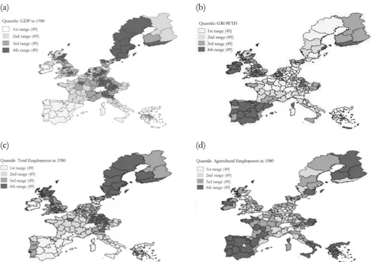
Creating maps which showed the spatial distribution of the considered vari-ables was a useful way of highlighting the potential spatial pattern of the observa-tions (figure 1). The spatial distribution of the regional per capita GDP in 1980 suggests that there was spatial heterogeneity, with two clusters of richer and poorer regions. The hypothesis that the geographical and economic peripheries substantially coincide is thus supported by this result. Spatial heterogeneity is also evident with regards to the other variables considered in the model: growth of per capita GDP between 1980 and 2006, regional employment rate and regional share of agricultural employment. Maps shown in figure 1 (panels a and b) also support the classical convergence hypothesis which associates a higher growth rate of per capita GDP to lower initial levels of per capita GDP.
(a) (b)
(c) (d)
Figure 1 – Spatial percentile distribution for the log of per capita GDP in 1980 with deviations with
respect to the EU-15 mean (a), the growth of per capita GDP between 1980 and 2006 (b), the total employment in 1980 (c), the share of agricultural employment in 1980 (d).
The spatial interaction between the regions is modelled, as usual in spatial analysis of lattice data, using the spatial weight matrix (W): a square, non-stochastic and symmetric matrix, whose elements (w ) measure the intensity of ij the spatial connection between regions i and j and take on a finite and non-negative value. The appropriate W used in most of the literature on spatial econometrics in a European regional context is a distance-based matrix (Fingle-ton, 1999; Baumont et al., 2001; Ertur et al., 2006; Le Gallo and Dall’Erba, 2006; Dall’Erba and Le Gallo, 2008; Ramajo et al., 2008), where each w is defined as ij
*/ * ij ij j ij w w
w and * * 2 * 0 1/ 0 ij ij ij ij ij ij w if i j w d if d D w if d D where * ijw is an element of the non-standardised spatial weights matrix; wij is an element of the standardised matrix (W); dij is the great circle distance between regions i and j; and D is the cut-off parameter above which any interaction between the regions is considered to be negligible; in this case it is defined as a quartile of the great circle distance distribution2. Standardising the spatial weight matrix does not influence the relative dependence between neighbours, but it makes it easier to interpret and compare the results of the calculations in which the matrix is used and also the results of different analyses.
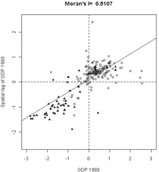
Relative to the variable per capita GDP in 1980, the Moran’s I index (Moran, 1950) is 0.5107, which is well above the expected value under the null hypothesis of no spatial correlation, E(I)=-0.0051. Initial per capita GDP is therefore spa-tially correlated and a positive spatial dependence is revealed in the distribution of this variable. A similar result was obtained for the GDP per capita growth rate between 1980 and 2006, leading to I= 0.2131. Another explorative analysis index of spatial autocorrelation (APLE; Li et al., 2007) confirms the existence of a posi-tive spatial autocorrelation. All these results are coherent to the choice of the weighting matrix.
Another explorative tool is the “Moran” scatterplot: each quadrant corre-sponds to a particular kind of spatial association between a region and its neighbours. The first and third quadrant display the situations of positive de-pendence between, respectively, the high/low values of the variable in one region and those in its neighbours. The second and fourth quadrant, on the other hand, show negative dependence. Thus from the Moran scatterplot one can identify
2 Here we present the results obtained by fixing the upper quartile of the distribution as the
cut-off parameter. We also used binary matrices (queen contiguity matrices and k-nearest neighbours spatial weights matrices for k=5 and k=10). The results generated by these other matrices are very similar to those presented in this paper.
whether or not there is spatial heterogeneity in the sample. The Moran scatterplot for per capita GDP in 1980 (figure 2) show two distinct clusters, one made up of rich regions surrounded by other rich regions (first quadrant) and the other of poor regions surrounded by poor regions (third quadrant).
Figure 2 – Moran scatterplot for the logarithm of per-capita GDP in 1980. Objective 1 regions are
identified by triangles, non-Objective 1 regions otherwise.
As a conclusion to the exploratory spatial analysis, a model is proposed that identifies two convergence clubs following the assumption of conformity be-tween geographical and economic periphery in the European Union. The crite-rion for the detection of the spatial regimes is therefore the economically-defined eligibility of each region to Objective 1 of the European regional policy: the first regime includes 50 NUTS-2, which were part of Objectives 1 and 6 during the programming period 1994-19993 (which are also identified by triangles in figure 2), the second regime includes the other 146 regions in the sample. All the re-gions that were granted the Funds for Objectives 1 and 6 during the program-ming period 1994-1999 are considered to be part of the Objective 1 cluster in the
3 We chose these dates so as to include Austrian, Swedish and Finnish regions in our analysis.
These countries joined the EU in 1995 and took part to the assignment of Structural Funds only from that programming period on. For a detailed list of the regions which were eligible to Objec-tives 1 and 6 during the programming period 1994-1999, see Council Regulation (EEC) No 2081/93 and Council Decision of 1 January 1995 in respect to adjusting the instruments concerning the accession of new member states to the European Union.
present analysis, although they might have been phased out in the following years. In accordance with the findings in literature (Ramajo et al. 2008), this distinction is expected to be suitable for modelling the possible spatial heterogeneity in the sample. Indeed it is well-known that in Europe economic disadvantages are usu-ally accompanied by geographical disadvantages (the term “European periphery” commonly indicates the poorest European regions). During the programming pe-riod 2000-2006, Objective 1 covered the former Objective 6 regions and the most remote regions, as well as those where development was lagging behind (Reg. 1260/99 EC). This reflects the EU’s awareness of the relationship between the geographical and the economic periphery. This hypothesis is also confirmed by the results of the exploratory spatial analysis. Any parameter instability between the two groups of regions that were exogenously defined will be considered to be proof of the existence of two convergence clubs with both a spatial and an eco-nomic dimension.
4. A CONVERGENCE MODEL AND SPATIAL EFFECTS AMONG EU REGIONS 4.1. The model of conditional β-convergence and spatial effects
The choice of the best model specification, in accordance with the results of the exploratory spatial analysis, follows the usual steps for model construction in spatial econometrics (Anselin, 2005).
Firstly, a model of conditional β-convergence without spatial effects (3) is es-timated via OLS:
y ybXθ ε
(3)
where y is a column vector with 196 observations for the rate of growth of per capita GDP in EU regions for the period 1980-2006, expressed in logarithms and in deviations with respect to the EU-15 mean; y is a column vector with 196 ob-servations for the level of per capita GDP in 1980, expressed in logarithms and in deviations with respect to the EU-15 mean; X [1 c 1 c ]2 is a 196x3 matrix where the first column permits to include the intercept, c1 is a column vector re-ferred to the total employment rate in each region in 1980, c2 is the column con-taining data for agricultural employment in each region in 1980; θ[a 1 2] and b are the regression coefficients; ε is the column vector of errors with the usual properties. For the sake of coherence with the definition of β-convergence models, the vector y was not included in the matrix X , which contains the vec-tors of the intercept and the covariates. The results of the OLS estimation of model (3), here not reported, show that each of the explanatory variables in-cluded is statistically significant and that they support the neoclassic assumption of conditional convergence. Moreover, since the the Breusch-Pagan test on the residuals does not rejected the hypothesis of homoskedasticity (p-value=0.374),
parameters instability was thought to be the most suitable tool to account for the spatial heterogeneity found through the exploratory spatial analysis.
Second step consists in testing for spatial autocorrelation in the regression re-siduals (Anselin, 1988; Anselin et al., 1996). The Moran’s I test statistic adapted to regression residuals rejects the hypothesis of no spatial autocorrelation for all cut-off distances, without providing any additional information on the best specifica-tion to choose (table 2).
TABLE 2
Moran’s I test for global spatial autocorrelation
Q1
(554 km) (p-value) (1044 km) Median (p-value) (1597 km) Q3 (p-value) Moran’s I test 0.1142 (0.017) 0.0996 (0.001) 0.0903 (0.000)
In order to choose the more appropriate spatial model, four Lagrange Multi-plier (LM) tests (Anselin, 1988, Anselin et al., 1996) are performed and the results are collected in table 3.
TABLE 3
Lagrange Multiplier tests for global spatial autocorrelation
Test (554 km) Q1 (p-value) (1044 km) Median (p-value) (1597 km) Q3 (p-value) LMlag test 6.3514 (0.012) 10.352 (0.001) 12.1379 (0.000) LMerr test 3.4991 (0.061) 7.3779 (0.007) 8.026 (0.005) RLMlag test 3.9643 (0.046) 2.9777 (0.084) 4.1439 (0.042) RLMerr test 1.112 (0.292) 0.0036 (0.953) 0.032 (0.858)
The results of the LM tests led to choose the spatial weights matrix based on third quartile, following Anselin’s suggestion (Ertur et al., 2006) to choose the cut-off distance which maximises the absolute value of the significant Lagrange mul-tiplier statistic for spatial autocorrelation. The LMlag test is more statistically sig-nificant than the LMerr (p-value=0.000 for the LMlag test and p-value=0.005 for the LMerr test), the RLMerr test is not significant (p-value=0.858) and the RLMlag is statistically significant at the 5% level (p-value=0.042). For the reasons above, a spatial lag model, or spatial auto-regressive model (SAR) is best for modelling the identified spatial dependence.
The spatial heterogeneity identified in subsection 3.2 is modelled by using two convergence clubs, defined according to both geographical and economic criteria. Using the estimates of a β-convergence model with two convergence clubs per-mits to have two spatial regimes with two distinct convergence processes, and also means that, thanks to the inclusion of conditioning variables, each regional economy inside each group of regions converges towards its own steady state. Following Ramajo et al. (2008), the spatial lags of the explanatory variables were included in the model specification as in a cross-regressive spatial model, but only the spatial lag of initial GDP was found to be significant. The final model is chosen by referring to the usual AIC and the log-likelihood value.
Let define the 196x196 diagonal matrix 1 ( ( i 1); 1,...,196) OB region OB diag i D I
that permits to select the regions belonging to Objective 1 (OB1), and
analo-gously 1 1
196 OB OB
d D 1 is the column vector used to select regions belonging to OB1. In the model proposed, y is a 196-dimensional column vector containing the per capita GDP in 1980, expressed in logarithms and in deviations with re-spect to the EU-15 mean. The 196x4-dimensional matrix of covariates
1 2 3
X [1 c c c ] contains respectively: in the first column unit values in or-der to include an intercept, in c1 the total employment rate in each region in 1980, in c2 the share of agricultural employment in of each region in 1980 and finally in c3 the spatial lag of y. By using DOB1 we obtain XOB1D XOB1 , and
1 1
196 196
( )
NN ' OB
X 1 1 D X. By considering vector dOB1, yOB1dOB1y and
1 1
196
( )
NN OB
y 1 d y are analogously obtained.
Then the chosen model, for y i.e. the rate of growth of per capita GDP in EU regions for the period 1980-2006, expressed in logarithms and in deviations with respect to the EU-15 mean; is:
1 1 1 1 1 1 1 1
OB OB NN NN OB OB NN NN
y y b y b X θ X θ Wgy ε
(4)
where θOB1
, θNN1 are the 4-dimensional vectors parameters, '
1 2
[ ]
i ai i i i
θ respectively for regions belonging to Objective 1
(i=OB1) and the others (i=NN1). Parameters bOB1, bNN1 are coefficients of the per capita GDP in 1980; is the spatial regression coefficient; W is the spatial weight matrix; ε is the column vector of errors with the usual properties.
The estimation results for model (4) are shown in the right-hand section of ta-ble 4, together with the results of the ML estimation of a model with no spatial regimes (left-hand section) which is included for comparison purposes.
TABLE 4
ML estimation results
Variable/parameter No convergence clubs (p-value) Objective 1 (p-value) non-Objective 1 (p-value) Constant (a) -0.00758 (0.011) -0.00312 (0.460) -0.01505 (0.000) GDP (b) -0.01735 (0.000) -0.02824 (0.000) -0.01569 (0.000) Total Employment (ψ1) 0.00026 (0.000) -0.00002 (0.846) 0.00043 (0.000)
Share of Agricultural Employment (ψ2) -0.00030 (0.000) -0.00029 (0.000) -0.00019 (0.037)
W_GDP (φ) 0.00304 (0.245) 0.02282 (0.000) -0.00521 (0.089) Spatial Parameter (ρ) 0.40931 (0.000) 0.35186 (0.001)
Convergence rate (β) % 2.3 5.3 2.0
Half life (years) 40 24.5 44
Breusch-Pagan test 4.432 (0.351) 13.5457 (0.139)
LMerr test 0.781 (0.377) 2.8226 (0.093)
Log likelihood 740.58 746.04
Chow test 47.01 (0.000)
4.2. Conditional β-convergence and spatial effects among EU-15 regions
The results of the ML estimation of model (4) support the assumption that there are two spatial convergence clubs, since the value of the Chow test rejects the null hypothesis of parameter stability between the two groups of regions. The choice of the model with spatial regimes is also supported by the usual AIC and log-likelihood values.
The model with no convergence clubs, which does not allow for parameter in-stability across space, appears to cause a loss of information if compared to the results of model (4). The estimated convergence rate is quite low (2.3%) and very close to that estimated for non-Objective 1 regions via model (4). The estimates of b obtained via model (4) are statistically significant and have the expected nega-tive sign. The implied convergence rate (β) of Objecnega-tive 1 regions (5.3%) is much higher than that of the other group (2%) and the half-life of the first group (24.5 years) is much lower than that of the second (44 years). As a result it seems to be advisable to estimate a SAR model with two spatial regimes. The choice of policy-defined exogenous clusters is supported by these results.
The assessment of two groups of regions converging at different rates towards different steady states is confirmed by the estimation of an unconditioned spatial error model (here not shown). Objective 1 regions appear to converge at a sig-nificantly higher rate than non-Objective 1 regions, irrespective of whether or not the spatial lag of GDP is included in the unconditioned model specification.
Although the existence of a convergence process across European regions is confirmed by some results in the literature, their comparison should be made with great caution, because some elements such as the time span considered, the estimation procedures and model specification may influence the estimates4, as it was made clear by Piras et al. (2006).
The estimate of the spatial parameter (ρ) confirms the crucial role of geogra-phy in explaining the economic growth. A β-convergence model with spatial ef-fects reveals that there are significant spillover efef-fects between European regions, and that these affect the economic performance of each of them. This result agrees with those of other studies (López-Bazo et al., 2004; Baumont et al., 2001; Ramajo et al., 2008). The more dynamic and fast growing the economies of the surrounding regions are, then the higher the growth rate of a region will be.
There is evidence that a high total employment rate has, on average, a signifi-cant positive influence on the growth of non-Objective 1 regions. The estimates of the share of those employed in agriculture reveal that there is an inverse rela-tionship between the importance of the agricultural sector and economic growth. In fact in both groups of regions the estimates of ψ2 are negative and significant at 5% level. In general, the initial self-employment rate is more important in richer regions, while the economic growth of Objective 1 regions is affected more by the initial share of self-employment in agriculture. Finally, the GDP of
4 See, for example, López-Bazo et al. (2004) for a spatial cross-sectional model; Esposti and
Bus-soletti (2010) for a non-spatial dynamic panel data model; Piras and Arbia (2007) for a spatial panel data model.
neighbouring regions has a positive effect on the growth of Objective 1 regions (0.023). The poorest regions, whose per capita GDP is less than 75% of the Community average, are the ones that are most affected by the economic situa-tions of their neighbours.
4.3. Policy implications
The main findings of this analysis are that development is polarised into two convergence clubs (Objective 1 and non-Objective 1 regions), and that these converge at different rates (respectively 5.3% and 2%) towards different steady states. As a result it is important to recognise that there will be permanent per capita income disparities between the two groups of regions. The significance of the conditioning variables, which affect the steady state of each region, rein-forces this conclusion. The identification of two distinct spatial regimes also al-lowed to assess the different impact of the conditioning variables on growth in the two groups of regions. The spatial lag of per capita GDP is found to be highly relevant in explaining the rate of growth in those regions that are lagging behind. Objective 1 regions are evidently more affected by the surrounding economic environment than richer regions are. The inclusion of this variable also gave the best improvements in the goodness of fit of the model and the biggest differences in the estimates of b. The greater negative effects of a high initial share of agricultural self-employment in Objective 1 regions should also be borne in mind, while a high initial self-employment rate has a positive effect mainly in non-Objective 1 regions. The different contribution of the composi-tion of the productive system and of the employment rate to the regional eco-nomic growth should also be taken into great consideration when planning re-gional cohesion Policy.
A model of this kind cannot explicitly demonstrate the causal relationship be-tween a higher convergence rate among poorer regions and regional policy fund-ing. However one cannot fail to notice that Objective 1 regions receive a much higher share of the total amount of funding for regional policy than is their share of total EU-15 GDP. Indeed during the programming period 1989-1993 the re-gions where development lagged behind received 69.6% of Structural Funds, while they only contributed 11% of EU GDP. In 1994-1999 they were granted 68.5% of the Funds and produced 13% of total EU-15 GDP. Finally, during the period 2000-2006, Objective 1 regions were given 69.9% of Structural Funds and produced 10% of EU-15 GDP5. It can reasonably assumed that such a distribu-tion of aid contributed to the higher convergence rate among the poorest regions, and this supports the hypothesis that the regions with a lower level of initial per capita income will grow at a higher rate, thus generating convergence. The evi-dence from the literature concerning the use of Structural Funds expenditure data within a convergence approach for policy evaluation purposes is still
5 The data on the amount of funding are taken from European Commission (1996; 2001) and do
not include the funding of the Cohesion Fund. The data on the GDP of Objective 1 regions are taken from the Cambridge Econometrics Regional Database.
sial (Rodrìguez-Pose and Fratesi, 2004; Esposti and Bussoletti, 2008; Dall’Erba and Le Gallo, 2008; Muccigrosso, 2010) and closely related with the model speci-fication (cross-sectional or panel data models, spatial or non-spatial approach). Moreover, the availability of data on the actual expenditure of the Structural Funds allocated to each NUTS-2 is still seriously limited.
The parameters estimated for the spatial autoregressive term and for the spa-tially lagged GDP also reveal that there are geographical spillover effects which are of primary importance in explaining the economic growth of European re-gions. The relative geographical location of each region plays a key role in ex-plaining the structure of economic growth in the EU-15. These findings have profound implications for policy and suggest that specific investments aimed at exploiting the spillover effects are important, as close coordination between neighbouring regions is. The funding granted to Objective 1 regions will be more effective in terms of economic convergence as the cohesion policies as-sume an “area”, and not just a regional, dimension. It is important to avoid rep-licating the National Strategic Reference Frameworks on a regional scale, past-ing them into the Regional Operational Programmes without adaptpast-ing them to the real specific territorial needs. Greater coordination between regions which have similar structural characteristics or are geographically adjacent would allow more accurate detection of the strengths of each region. The concentration of resources on these different strengths (at a regional level) would also stimulate stronger spillover effects towards neighbours. Consequently, the policy-makers should take the crucial role of geographical spillover effects into account when planning economic policies.
5. CONCLUSIONS
The aim of this paper is to assess the economic convergence among EU-15 regions by estimating a conditional β-convergence model which takes into ac-count the effects of spatial dependence and spatial heterogeneity. Per capita GDP follows a spatial pattern: the highest values are found in the European geographical core, as the traditional “centre-periphery” models usually predict. This confirms the hypothesis that the economic and geographical periphery in Europe generally coincide. This analysis then employed a model which dis-criminates regions (Objective 1 vs. non-Objective 1 regions) in order to study the economic growth in these two policy-defined groups. This work can be considered as a starting point for constructing a model able to evaluate the ef-fects of cohesion policy.
Differently from the majority of previous studies (Dall’Erba and Le Gallo, 2006, 2008; Ertur et al., 2006; Rodríguez-Pose and Fratesi, 2004) that accounted for spatial heterogeneity through the identification of different convergence clubs, in this paper we chose to adopt an exogenous criterion for the definitions of the clubs. The spatial autocorrelation was also modelled. This added greatly to the value of the analysis, because the results highlighted some factors which are
not usually revealed by those studies which do not explicitly take spatial effects into account: Objective 1 regions are affected more by geographical spillovers and also converge faster to their steady state than do non-Objective 1 regions and per capita income disparities between the two groups of regions seem to be per-sistent.
The results of our analysis can be also considered from a policy-making point of view: the spatial spillovers and the different contributions of both the eco-nomic structure and the labour market to the growth of Objective 1 and non-Objective 1 regions should be taken into consideration when planning an effec-tive EU cohesion Policy.
Further possible developments of this analysis include the estimation of a spa-tial panel data model for considering the temporal dynamic of economic conver-gence together with the spatial one and the inclusion of data on Structural Funds expenditure among the conditioning variables, in order to better assess the effects of European Cohesion Policy on economic growth.
APPENDIX TABLE A.1
List of NUTS-2 non-Objective 1 regions included in the sample
Code Region Code Region
AT12 Niederösterreich FR53 Poitou-Charentes
AT13 Wien FR61 Aquitaine
AT21 Kärnten FR62 Midi-Pyrénées
AT22 Steiermark FR63 Limousin
AT31 Oberösterreich FR71 Rhône-Alpes
AT32 Salzburg FR72 Auvergne
AT33 Tirol FR81 Languedoc-Roussillon
AT34 Vorarlberg FR82 Provence-Alpes-Côte d’Azur BE10 Région de Bruxelles-Capitale ITC1 Piemonte
BE21 Antwerpen ITC2 Valle d’Aosta/Vallée d’Aoste
BE22 Limburg (B) ITC3 Liguria
BE23 Oost-Vlaanderen ITC4 Lombardia
BE24 Vlaams Brabant ITD1 Provincia Autonoma Bolzano-Bozen BE25 West-Vlaanderen ITD2 Provincia Autonoma Trento
BE31 Brabant Wallon ITD3 Veneto
BE33 Liège ITD4 Friuli-Venezia Giulia
BE34 Luxembourg (B) ITD5 Emilia-Romagna
BE35 Namur ITE1 Toscana
DE11 Stuttgart ITE2 Umbria
DE12 Karlsruhe ITE3 Marche
DE13 Freiburg ITE4 Lazio
DE14 Tübingen LU00 Luxembourg
DE21 Oberbayern NL11 Groningen
DE22 Niederbayern NL12 Friesland
DE23 Oberpfalz NL13 Drenthe
DE24 Oberfranken NL21 Overijssel
DE25 Mittelfranken NL22 Gelderland
DE26 Unterfranken NL31 Utrecht
DE27 Schwaben NL32 Noord-Holland
DE50 Bremen NL33 Zuid-Holland
DE60 Hamburg NL34 Zeeland
DE71 Darmstadt NL41 Noord-Brabant
DE72 Gießen NL42 Limburg (NL)
DE73 Kassel SE11 Stockholm
DE91 Braunschweig SE12 Östra Mellansverige
DE92 Hannover SE21 Småland med öarna
DE93 Lüneburg SE22 Sydsverige
DE94 Weser-Ems SE23 Västsverige
DEA1 Düsseldorf UKC1 Tees Valley and Durham DEA2 Köln UKC2 Northumberland, Tyne and Wear
DEA3 Münster UKD1 Cumbria
DEA4 Detmold UKD2 Cheshire
DEA5 Arnsberg UKD3 Greater Manchester
DEB1 Koblenz UKD4 Lancashire
DEB2 Trier UKD5 Merseyside
DEB3 Rheinhessen-Pfalz UKE1 East Riding and North Lincolnshire
DEC0 Saarland UKE2 North Yorkshire
DEF0 Schleswig-Holstein UKE3 South Yorkshire
DK01 Hovedstadsreg UKE4 West Yorkshire
DK02 Øst for Storebælt UKF1 Derbyshire and Nottinghamshire DK03 Vest for Storebælt UKF2 Leicestershire, Rutland and Northants
ES21 Pais Vasco UKF3 Lincolnshire
ES22 Comunidad Foral de Navarra UKG1 Herefordshire, Worcestershire and Warks ES23 La Rioja UKG2 Shropshire and Staffordshire
ES24 Aragón UKG3 West Midlands
TABLE A.2
List of NUTS-2 Objective 1 regions included in the sample
Code Region Code Region
AT11 Burgenland GR25 Peloponnisos
BE32 Prov. Hainaut GR30 Attiki
ES11 Galicia GR41 Voreio Aigaio
ES12 Principado de Asturias GR42 Notio Aigaio
ES13 Cantabria GR43 Kriti
ES41 Castilla y León IE01 Border, Midlands and Western ES42 Castilla-la Mancha IE02 Southern and Eastern
ES43 Extremadura ITF1 Abruzzo
ES52 Comunidad Valenciana ITF2 Molise
ES61 Andalucia ITF3 Campania
ES62 Región de Murcia ITF4 Puglia
ES63 Ciudad Autónoma de Ceuta (ES) ITF5 Basilicata ES64 Ciudad Autónoma de Melilla (ES) ITF6 Calabria
FI13 Itä-Suomi ITG1 Sicilia
FI19 Länsi-Suomi ITG2 Sardegna
FI1A Pohjois-Suomi PT11 Norte
FR83 Corse PT15 Algarve
GR11 Anatoliki Makedonia, Thraki PT16 Centro (PT)
GR12 Kentriki Makedonia PT17 Lisboa
GR13 Dytiki Makedonia PT18 Alentejo
GR14 Thessalia SE31 Norra Mellansverige
GR21 Ipeiros SE32 Mellersta Norrland
GR22 Ionia Nisia SE33 Övre Norrland
GR23 Dytiki Ellada UKM6 Highlands and Islands GR24 Sterea Ellada UKN0 Northern Ireland
Figure A.1 – Maps of NUTS-2 non-Objective 1 regions included in the sample (left-hand panel) and
Objective 1 regions included in the sample (right-hand panel).
Dipartimento di Scienze Statistiche CRISTINA BRASILI
Università di Bologna FRANCESCA BRUNO
REFERENCES
L. ANSELIN, (1988), Spatial Econometrics: Methods and Models. Dordrecht, Boston, London:
Kluwer Academic Publishers.
L. ANSELIN, A. K. BERA, R. FLORAX, M. J. YOON, (1996), Simple diagnostic tests for spatial dependence,
Regional, “Science and Urban Economics”, 26, pp. 77-104.
L. ANSELIN, (2005), Exploring Spatial Data with GeoDa: A Workbook, Centre for Spatially
In-tegrated Social Sciences.
G. ARBIA, (2006), Spatial Econometrics. Berlin Heidelberg, Springer-Verlag.
G. ARBIA, M. BATTISTI, G. DI VAIO, (2010), Institutions and geography: Empirical test of spatial growth
models for European regions, “Economic Modelling”, vol. 27, 1, pp. 12-21.
R. J. BARRO, (1991), Economic Growth in a Cross Section of Countries, “The Quarterly Journal of
Economics”, Vol. 106, No. 2, pp. 407-443.
R. BARRO, X. SALA-I-MARTIN, (1991), Convergence across states and regions, “Brookings Papers on
Economic Activity”, pp. 107-182.
R. BARRO, X. SALA-I-MARTIN, (1992), Convergence, “Journal of Political Economy”, 100, pp.
223-251.
R. BARRO, X. SALA-I-MARTIN, (1995), Economic Growth. McGraw-Hill, Inc.
M. BATTISTI, G. DI VAIO, (2008), A spatially filtered mixture of β-convergence regressions for EU
re-gions, 1980-2002, “Empirical Economics”, 34, pp. 105-121.
W. J. BAUMOL, (1986), Productivity Growth, Convergence, and Welfare: What the Long-Run Data
Show, “The American Economic Review”, vol. 75, n. 5, pp. 1072-1085.
C. BAUMONT, C. ERTUR, J. LE GALLO, (2001), A Spatial Econometric Analysis of Geographic Spillovers
and Growth for European Regions, 1980-1995, Working Paper n.2001-04, LATEC UMR-CNRS 5118, Université de Bourgogne.
K. J. BUTTON, E. J. PENTECOST, (1999), Regional Economic Performance within European Union,
Cheltenham, Edward Elgar.
COUNCIL REGULATION (EC) 2081/93. COUNCIL REGULATION (EC) 1260/99. COUNCIL REGULATION (EC) 1083/06.
S. DALL’ERBA, J. LE GALLO, (2008), Regional Convergence and the Impact of European Structural
Funds over 1989-1999: A Spatial Econometric Analysis, “Papers in Regional Science”, vol. 87, n. 2, pp. 219-244.
C. ERTUR, J. LE GALLO, C. BAUMONT, (2006), The European Regional Convergence Process,
1980-1995: Do Spatial Regimes and Spatial Dependence Matter?, “International Regional Science Review”, vol. 29, pp. 3-34.
R. ESPOSTI, S. BUSSOLETTI, (2008), Impact of Objective 1 Funds on Regional Growth Convergence in the
European Union: A Panel-data Approach, “Regional Studies”, vol. 42, n. 2, pp. 159-173.
EUROPEAN COMMISSION, (1996), First report on economic and social cohesion. Luxembourg, Office
for Official Publications of the European Communities.
EUROPEAN COMMISSION, (2001), Second report on economic and social cohesion. Luxembourg,
Of-fice for Official Publications of the European Communities.
B. FINGLETON, (1999), Estimates of Time to Economic Convergence: An Analysis of Regions of the
European Union, “International Regional Science Review”, 22, pp.5-34.
J. P. FITOUSSI, (2006), Democrazia e Mercato in “Argomenti”, n° 17, pp. 5-11.
A.O. HIRSCHMAN, (1958), The Strategy of Economic Development, New Haven, Yale University
Press.
P. KRUGMAN, (1991), Geography and Trade. Cambridge, MIT Press.
Convergence Process, 1980-1999, “Journal of Regional Science”, Vol. 46, n. 2, 2006, pp. 269-288.
R. LEONARDI, (1995), Convergence, cohesion and integration in the European Union. New York, St.
Martin’s Press.
H. LI, C. A. CALDER, N. CRESSIE, (2007), Beyond Moran’s I: Testing for Spatial Dependence Based on
the Spatial Autoregressive Model, “Geographical Analysis”, 39, pp. 357-375.
E. LÓPEZ-BAZO, E. VAYÀ, A. J. MORA, J. SURIÑACH, (1999), Regional economic dynamics and convergence
in the EU, “The Annals of regional Science”, 33, pp. 343-370.
E. LÓPEZ-BAZO, E. VAYÀ, M. ARTIS, (2004), Regional Externalities and Growth: Evidence from
Euro-pean Regions, “Journal of Regional Science”, 44, pp. 43-73.
P.A.P. MORAN, (1950), Notes on Continuous Stochastic Phenomena, “Biometrika”, 37, pp. 17-33. T. MUCCIGROSSO, (2010), I fattori della crescita regionale nell’Unione europea. Un modello basato sulla
spesa per le politiche, “Rivista economica del Mezzogiorno”, n. 1-2, pp. 141-178.
G. MYRDAL, (1957), Economic Theory and Underdeveloped Regions, Gerald Duckworth, London. G. OTTAVIANO, D. PUGA, (1998), Agglomeration in the Global Economy: A Survey of the New
Eco-nomic Geography, “The World Economy”, 21(6), pp. 707-731.
G. PIRAS, G. ARBIA, J. LE GALLO, (2006), A meta analysis of regional economic convergence of the
NUTS-2 European regions, 1977-2002, paper presented at the 45th European Congress of the European Regional Sciences Association (ERSA).
G. PIRAS, G. ARBIA, (2007), Convergence in per-capita GDP across EU-NUTS2 regions using panel
data models extended to spatial autocorrelation effects, “Statistica”, anno LXVII, n. 2, pp. 157-172.
J. RAMAJO, M. A. MARQUEZ, G. J. D. HEWINGS, M. M. SALINAS, (2008), Spatial Heterogeneity and
Re-gional Spillovers in the European Union: Do cohesion policies encourage convergence across regions?, “European Economic Review”, n. 52, pp. 551-567.
A. RODRÍGUEZ-POSE, U. FRATESI, (2004), Between Development and Social Policies: The impact of
European Structural Funds in Objective 1 Regions, “Regional Studies”, 38:1, pp. 97-113.
X. SALA-I-MARTIN, (1996), The Classical Approach to Convergence Analysis, “The Economic
Jour-nal”, vol. 106, n. 437, pp. 1019-1036.
SUMMARY
A spatial econometric approach to EU regional disparities between economic and geographical periphery A conditional β-convergence model and a distance-based weight matrix are used to analyse the economic convergence among European NUTS-2 regions over the period 1980-2006. A Spatial Autoregressive Model which identifies two spatial regimes and spa-tial dependence finds that the convergence process among EU regions is affected by po-larization into two clusters defined both on a geographical and economic criterion, which converge at different rates towards different steady states.
This result confirms the hypothesis that a methodology which uses spatial econometric techniques is needed to model spatial effects, and that otherwise the estimates are likely to be inefficient or even biased.