A Data-driven Approach to Construct Survey-based Indicators by
Means of Evolutionary Algorithms
Oscar Claveria¹*, Enric Monte², Salvador Torra³
¹ AQR-IREA, University of Barcelona (UB)
² Department of Signal Theory and Communications, Polytechnic University of Catalunya (UPC) ³ Riskcenter-IREA, Department of Econometrics and Statistics, University of Barcelona (UB)
Acknowledgements
This paper was supported by by the project ECO2016-75805-R of the Spanish Ministry of Economy and Competitiveness. We would like to thank two anonymous referees for their useful comments and suggestions. We also wish to thank Johanna Garnitz and Klaus Wohlrabe at the Ifo Institute for Economic Research in Munich for providing us the data used in the study.
* Corresponding Author:
1 Introduction
Tendency surveys ask agents about whether they expect a variable to rise, to fall, or to remain unchanged. Individual answers are aggregated as percentages of the respondents in each category. The qualitative nature of survey results has led to quantify agents’ responses by means of survey indicators. The most used indicator to present survey results is the balance statistic. Anderson (1951, 1952) defined the balance statistic as the difference between the percentage of agents reporting an increase and the percentage reporting a decrease. As the balance statistic does not take into account the percentage of respondents expecting a variable to remain unchanged, Claveria (2010) proposed a variation of the balance statistic that accounts for the percentage of respondents reporting a “no change”, and therefore allows discriminating between two equal values of the balance statistic depending on the percentage of respondents expecting a variable to remain constant. By matching firm-level responses and outcomes, Müller (2010) found that the median of the “no change” category was equal to zero. Abberger (2007) used probit analysis to estimate a quantitative threshold for employment expectations that allows to differentiate between a decrease and an increase in actual employment. Van den Berg et al. (2006) discussed implications for standard methods to deal with non-response bias.
The balance statistic has been widely used to test economic hypothesis (Girardi 2014; Jean-Baptiste 2012, Zárate et al. 2012; Schmeling and Schrimpf 2011; Jonsson and Österholm 2011, 2012; Paloviita 2006; Pesaran and Weale 2006; Lemmens et al. 2005 2008; Pehkonen 1992; Ivaldi 1992; Batchelor and Dua 1992; Ilmakunnas 1989; Pesaran 1984, 1985, 1987). Balances have also been used as explanatory variables in economic models (Altug and Çakmakli 2016; Guizzardi and Stacchini 2015; Martinsen et al. 2014; Ghonghadze and Lux 2012; Robinzonov et al. 2012; Lui et al. 2011a, 2011b; Schmeling and Schrimpf 2011; Franses et al. 2011; Klein and Özmucur 2010; Graff 2010; Claveria et al. 2007; Abberger 2007; Mitchell et al. 2005a; Hansson et al. 2005; Mittnik and Zadrozny 2005; Batchelor and Dua 1998; Kauppi et al. 1996; Parigi and Schlitzer 1995; Bergström 1995; Rahiala and Teräsvirta 1993; Biart and Praet 1987).
The balance statistic can be regarded as a qualitative measure of the average changes expected in a variable. As a result, numerous methods to transform balances into quantitative indicators have been proposed in the literature. Based on the assumption that
respondents report a variable to go up (or down) if the mean of their subjective probability distribution lies above (or below) a threshold level, Theil (1952) proposed the probability approach. This threshold is known as the indifference interval. Carlson and Parkin (1975) applied the method by using a normal distribution together with symmetric and constant threshold parameters across respondents and over time. Extensions of this framework are mainly focused on reducing the measurement error introduced by incorrect assumptions (Lahiri and Zhao 2015; Breitung and Schmeling 2013; Mitchell et al. 2002; Löffler 1999; Berk 1999; Smith and McAleer 1995; Dasgupta and Lahiri 1992; Kariya 1990; Batchelor and Orr 1988; Seitz, 1987; Pesaran 1984; Batchelor 1982, 1986; Toyoda 1979). By means of Monte Carlo simulations, Terai (2009) and Löffler (1999) estimated the measurement error introduced by the probabilistic method. See Vermeulen (2014), Driver and Urga (2004), and Nardo (2003) for a review of the different quantification methods.
Matching firm-level responses to quantitative realizations, several authors have also developed extensions of the probability approach. In a recent study, Lahiri and Zhao (2015) have proposed a generalization of the probability approach that allows time-varying and heterogeneous thresholds. Müller (2010) developed a variant of the probability method assuming asymmetric and time invariant thresholds based on the “conditional absolute null” empirical property that the median of realized quantitative values corresponding to the “no change” category is zero. The main advantage of this procedure is that it solved the zero response problem. Also based on firm-level responses, Mitchell et al. (2002) developed a survey-based indicator. For an appraisal of individual firm data on expectations see Zimmermann (1997).
Agents’ responses are also used to construct composite indicators based on survey results. Examples are the Consumer Confidence Indicator (Białowolski 2015; Gelper et al. 2007), and the Economic Sentiment Indicator (Gelper and Christophe 2010) constructed by the European Commission (European Economy, 2014) by aggregating the sectoral indicators (Frale et al. 2010; Taylor and McNabb 2007). Re-scaling individual replies by means of a grading procedure, the Ifo Institute for Economic Research elaborate the Economic Climate Index (ECI) (CESifo World Economic Survey, 2011), which is an aggregate indicator obtained as the arithmetic mean of two questions from the World Economic Survey (WES). Camacho and Perez-Quiros (2010) used the Ifo Business Climate Index (IBCI) and the ESI to forecast economic growth in the Euro-area. Robinzonov et al. (2012) used the IBCI and other aggregate indicators from surveys as exogenous variable for industrial production forecasting.
There are many studies analysing the relationship between survey data and macroeconomic variables (Mokinski et al. 2015; Dees and Brinca 2013; Leduc and Sill 2013; Lui et al. 2011a, 2011b; Zanin 2010; Gelper and Croux 2007, 2010; Claveria et al. 2007; Abberger 2007; Nolte and Pohlmeier 2007; Cotsomitis and Kwan 2006; Mitchell et al. 2005a, 2005b), but this is the first study to link both sources of information by means of symbolic regression (SR) to derive a leading economic indicator. As far as we know, this is the first attempt at designing an empirically generated SR-based indicator. We use genetic programming (GP) to infer building blocks that relate the answers of the surveys to the actual evolution of GDP. This data-driven approach allows to identify the optimal combinations of a wide range of survey variables that best fits the evolution of GDP.
In this study we aim to break new ground by presenting a novel method to design data-driven composite indicators. We use quarterly survey data from the WES to construct an economic indicator to track the evolution of GDP. The dataset is composed of twelve survey variables for twenty-eight countries of the OECD. The proposed methodology is based on evolutionary computation and SR. Through Darwinian competition, the algorithm derives a set of mathematical functional forms that approximate a predefined target variable. These models of interaction between variables can be regarded as the set of the fittest empirically-generated indicators, which are in turn used as building blocks to construct a survey-based economic indicator.
The structure of the paper is as follows. Section 2 describes the data and our methodological approach. In Section 3 we present the empirical results. Finally, conclusions are given in Section 4.
2 Data and Methods
In this study we link agent’s expectations from the WES in 28 countries of the OECD to year-on-year growth rates of real GDP for the period comprised between the second quarter of 2000 and the first quarter of 2014. The WES assesses worldwide economic trends by polling professionals and experts on current economic developments in their respective countries (Kudymowa et al. 2013). Białowolski (2016) points out that professional respondents are characterized by significantly lower biases in responding to survey questions than consumers, who are prone to a negative response pattern.
Respondents are asked to express their present judgement, their assessment compared to the same time last year, and their expectation by the end of the next six months with respect to a wide range of variables (capital expenditures, private consumption, foreign trade, inflation, interest rates, share prices, etc.).
The Ifo uses a grading procedure consisting in assigning a grade of nine to positive replies, of five to indifferent replies, and of one to negative replies. This procedure is conceptually equal to calculating balances. Aggregation is based on country classifications, so that the country results are weighted according its share of exports and imports in total world trade (CESifo World Economic Survey, 2011). Henzel and Wollmershäuser (2005), Stangl (2007, 2008) and Hutson et al. (2014) provide a detailed analysis of WES data.
In this study we use the Ifo statistic with respect to twelve variables: The judgement about the present economic situation regarding:
o the overall economy ( 1x )
o capital expenditures ( 2x )
o private consumption ( 3x ).
The assessment of the economic situation compared to the same time last year regarding:
o the overall economy ( 4x )
o capital expenditures ( 5x )
o private consumption ( 6x )
The expected economic situation by the end of the next six months regarding: o the overall economy ( 7x )
o capital expenditures ( 8x )
o private consumption ( 9x )
o exports ( 10x ) o imports ( 11x )
o balance of trade ( 12x )
The ECI is an aggregate indicator obtained as the arithmetic mean of assessments of the general economic situation and the expectations for the economic situation in the next six months. The ECI tends to correlate closely with the actual business-cycle trend measured in annual growth rates of real GDP (Garnitz et al., 2015). In Table 1 we present a descriptive analysis of the ECI for the ten European economies evaluated in this study.
Table 1 Descriptive statistics – ECI
mean standard
deviation
variation
coefficient (%) skewness kurtosis
Austria 5.30 1.07 20.2% -0.03 0.36 Belgium 5.14 1.09 21.1% -0.24 0.15 France 4.70 1.10 23.4% 0.04 -0.07 Germany 5.49 1.09 19.9% -0.03 -0.93 Greece 4.56 1.57 34.5% 0.67 0.25 Ireland 5.34 1.77 33.2% -0.36 -0.64 Italy 4.44 0.93 21.0% -0.09 -0.61 Netherlands 5.33 1.12 21.0% 0.26 -0.30 Portugal 3.84 1.22 31.7% -0.17 -0.50 Spain 4.39 1.34 30.4% -0.35 -1.01
The analysis conducted in this study links WES variables to GDP data retrieved from the OECD web (https://data.oecd.org/gdp/quarterly-gdp.htm#indicator-chart). We use year-on-year growth rates of quarterly GDP as a yardstick in order to derive
functional forms that can be regarded as proxies of economic growth. The model does not consider dynamics, and the goal is not prediction. The main objective of this research is to present a data-driven approach to design a composite survey-based
indicator. The proposed procedure allows us to identify a set of optimal combinations of a wide range of survey variables to track the evolution of GDP.
As there is an arbitrary functional relationship between the set of survey variables, we link them to the actual percentage growth rate of GDP by means of a SR model:
it it it it it it it it it it it it
it f x x x x x x x x x x x x
y 1 , 2 , 3 , 4 , 5 , 6 , 7 , 8 , 9 , 10 , 11 , 12
where x1 it, ,x12it are the WES variables as published by the Ifo, and yit is a scalar
referring to the year-on-year growth rate of quarterly GDP for country i at time t. SR is an empirical modelling approach that does not rely on a specific a priori determined model structure. SR finds the optimal combination of variables from a space of all algebraic expressions defined by a set of given operations and functions. Koza (1992) was the first to apply GP in the solution of SR problems. GP was developed by Cramer (1985), and can be regarded as an extension of genetic algorithms (GAs). GP belongs to the class of evolutionary algorithms (EAs), which were introduced by Holland (1975). See Zelinka (2015), Fogel (2006), and Goldberg (1989) for applications and a comprehensive overview.
Due to its flexibility, empirical modelling with SR is starting to be applied in economics. Kotanchek et al. (2010) used SR to detect outliers and identify models in large public datasets. Álvarez-Díaz and Álvarez (2005) made use of GP to generate predictions of exchange rates. Kronberger et al. (2011) used SR to estimate US inflation based on the identified variable interactions in a large dataset of economic indicators. Kľúčik (2012) combined SR with GP in the estimation of foreign trade to Slovakia. Acosta-González et al. (2012) apply GP to select the best econometric model for explaining the severity of the 2008 crisis. Yang et al. (2015) used SR to forecast oil production.
In this study we propose a method to construct survey-based indicators making use of a SR-based approach. By means of GP we infer a set of building blocks that relate the answers of the respondents to the evolution of GDP. The set of predetermined primitive functions limits the possible types of derived functional relationships. To simplify the analysis, we restricted the number of primitive functions on the survey variables to the mean, the maximum, the minimum, the ratio, and the logarithm. This set of functions are applied to the WES variables as they are published by the Ifo.
To control for the growth in complexity of the SR functions, we introduced a term that penalized the functions with a complexity in the cost function. We penalized the absolute number of terms on the expression. The penalization term can either be on the number of terms or on the depth of the syntactic trees. Empirically, we found that the restriction on the depth of the syntactic trees excluded reasonable solutions in which the concatenation of different functions had sense, so we decided to penalize the absolute number of terms on the expression. The penalization for expressions with more than 20 terms was linear with the number of terms, with a slope that was determined
heuristically as an increase of 10% in the error for each additional term. This procedure allowed us to obtain two or three levels of nested expressions.
As in one run of the GP algorithm the returned functions in the last generation tend to be highly correlated with each other, the selection process was undertaken in several independent runs of the simulation. On the one hand, components which had no
economic sense were rejected. On the other hand, using as a criterion the correlation coefficients between the elements of the population and the dependent variable, we selected the components present in the top elements of the estimated populations of five different runs. Finally, we linearly combined these building blocks to generate an indicator of economic growth. See Dabhi and Chaudhary (2015) for an overview of GP issues.
The implementation of GP for SR can be summarized in the following steps: 1. Creation of an initial population.- We determined a population size of 1000
programs.
2. Evaluation of fitness.- For each member of the population, an error metric is calculated. We used the Root Mean Square Error (RMSE) as a fitness function. 3. Selection for reproduction.- From the existing strategies for the selection of parents
for replacement, we used the tournament method so as to guarantee diversity in the population.
4. Application of genetic operators.- The main genetic operations are reproduction (copy), crossover (recombination of randomly chosen parts of parents), and mutation (randomly altering a part of a parent). Once the probability of a new generation (reproduction and mutation probabilities) is determined, operators are applied to the parents selected on the basis of the fitness function. We have selected a 0.1 probability.
5. Determination of constants.- GP can be complemented with an optimization of the set of constants after a number of generations to avoid the search path to deviate from the optimum, given by the best possible correlation relative to both functional form and the constants. We included the automatic generation of constants provided by the GA.
6. Creation of a new population.- Steps three and four are repeated until a new
generation is built. If no individual in the population has a required minimal fitness, or any other stopping criterion is fulfilled, everything is repeated from the second step onwards using the new generation as the population. Consequently, the fitness of the population is ever increasing. We have chosen a maximum number of 150 generations as as stopping criterion.
In this study we have used the open source Distributed Evolutionary Algorithms Package (DEAP) framework implemented in Python (Fortin et al. 2012; Gong et al. 2015).
3 Results
In this section we assess the output of the SR via GP. First, we present the set of selected building blocks from the GP experiment (Table 2).
Table 2 Building blocks 1 Log x4 8 11 12 x x 2 Log x5 9 12 11 10 x x x 3 Log x10 10 3 10 , 2 10 , 1 10 max x x x x x x Log 4 Log x12 5 5 2 x x 11 2 3 1 x x Log 6 6 3 x x 12 3 6 5 4 x x x Log 7 7 1 x x 13 3 9 8 7 x x x Log
These expressions, which can be regarded as proxies of economic growth, are linearly combined to construct a composite economic indicator. As we have used the same model for all countries, we compare the performance of the proposed indicator in ten European economies: Austria, Belgium, France, Germany, Greece, Ireland, Italy, the Netherlands, Portugal and Spain.
In Fig. 1 we compare the evolution of the proposed SR-based indicator to that of the
scaled CESIfo’s ECI and the year-on-year growth rates of GDP in the ten European economies analysed. Both indicators show a similar pattern of evolution. Nevertheless, we want to note that the the ECI is not tuned to fit the evolution of GDP. Regarding the differences across the analysed economies, we observe that in Belgium and Spain the survey-based indicator seems to lead turning points, especially with respect to the 2008 financial crisis. Part of this pattern could be attributed to the fact that official quantitative information on GDP is usually available with a delay with respect to survey information, and this effect was not accounted for. In the other eight countries, the co-movements between both series seem to be contemporary. As a rule, the proposed indicator seems to correlate closely with the actual oscillations of GDP.
Fig. 1. Evolution of year-on-year GDP growth rates vs. survey-based economic indicators Austria Belgium France Germany Greece Ireland Italy Netherlands Portugal Spain
1. Note: The black line represents the year-on-year growth rate of GDP in each country. The grey line represents the evolution of the scaled Ifo Economic Climate indicator. The black dotted line represents the evolution of the proposed indicator.
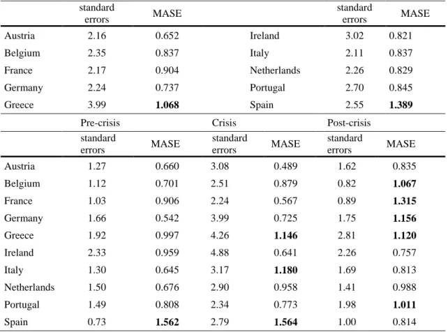
Next, we evaluate the performance of the proposed indicator to track the evolution of GDP. We use the Mean Absolute Scaled Error (MASE) statistic proposed by Hyndman and Koehler (2006), which scales the errors by the in-sample MAE obtained with a random walk. As survey data refer to expectations, and are available ahead of the publication of quantitative official data, we use two-step ahead naïve forecasts as a benchmark. The MASE is an accuracy measure independent of the scale of the data (Hyndman and Koehler 2006). Another advantage of the MASE is that it is easy to interpret: values larger than one are indicative that the survey-based indicator is outperformed by the average prediction computed in-sample with the benchmark model.
Table 3 Standard errors of estimations and MASE by country standard errors MASE standard errors MASE Austria 2.16 0.652 Ireland 3.02 0.821 Belgium 2.35 0.837 Italy 2.11 0.837 France 2.17 0.904 Netherlands 2.26 0.829 Germany 2.24 0.737 Portugal 2.70 0.845 Greece 3.99 1.068 Spain 2.55 1.389
Pre-crisis Crisis Post-crisis
standard errors MASE standard errors MASE standard errors MASE Austria 1.27 0.660 3.08 0.489 1.62 0.835 Belgium 1.12 0.701 2.51 0.879 0.82 1.067 France 1.03 0.906 2.24 0.567 0.89 1.315 Germany 1.66 0.542 3.99 0.725 1.75 1.156 Greece 1.92 0.997 4.26 1.146 2.81 1.120 Ireland 2.33 0.959 4.88 0.641 2.26 0.757 Italy 1.30 0.645 3.17 1.180 1.69 0.813 Netherlands 1.50 0.676 2.90 0.958 1.41 0.988 Portugal 1.49 0.808 2.34 0.773 1.98 1.011 Spain 0.73 1.562 2.79 1.564 1.00 0.814
Notes: * MASE stands for the Mean Absolute Scaled Error. In this study we propose scaling the errors by the in-sample MAE obtained with the Naïve method for two-step ahead forecasts (as official data are published with a delay of more than a quarter with respect to survey data). Values larger than one (in bold) indicate worse predictions than the average forecast computed in-sample with the Naïve method.
In Table 3 we observe differences in the performance of the proposed indicator across countries. Greece and Spain are the only economies in which the naïve model used as a benchmark outperforms the proposed indicator. Greece is the country that presents the highest standard errors.
Łyziak and Mackiewicz-Łyziak (2014) found that the crisis influenced the forecasting performance of survey-based measures. Hence, in order to assess the effect of the financial crisis on the accuracy of the proposed indicator, we re-compute the MASE differentiating between the pre-crisis subperiod (2000-2006), the crisis (2007-2010), and the post-crisis subperiod. When we divide the sample period in three subperiods, we observe a deterioration in the predictive performance of of survey-based measures of economic growth. The only two exceptions are Spain and Ireland, where there has been an improvement with respect to the pre-crisis period. During the crisis, standard errors are higher in all economies, being Ireland the country displaying the highest values, while Austria the one with the most accurate estimates with respect to the benchmark.
These results are in line with those of Białowolski (2015), who evaluated the consumer confidence indicator in Poland, and found that consistency of responses decreased in periods with more changes in the economic environment. The author proposed an alternative set of survey variables to calculate both indicators but did not find significant improvements in forecast accuracy.
However, our results contrasts with those obtained for Central and Eastern European economies by Claveria et al. (2016) and Łyziak and Mackiewicz-Łyziak (2014). Claveria et al. (2016) found an improvement in the capacity of agents’ expectations in ten Central and Eastern European countries to anticipate economic growth after the crisis. Similarly, Łyziak and Mackiewicz-Łyziak (2014) analysed twenty European countries, differentiating between advanced and transition economies, and found evidence that the 2008 financial crisis period led to a decrease in expectational errors in transition economies. Kauppi et al. (1996) found that the importance of business survey information increased during recession periods, as they obtained a significant improvement in prediction accuracy after taking account of relevant business survey information during Finland’s great depression.
4 Conclusions
Survey data on expectations is increasingly used to assess the current state of the economy. Survey expectations are based on the knowledge of the respondents operating in the market and provide detailed information about a wide range of variables. Many methods have been proposed to aggregate survey variables, nevertheless there is no
consensus on the most appropriated method. In this paper we present a data-driven approach to generate a survey-based indicator. This empirical method for aggregating expectational variables presents several advantages. On the one hand, the proposed indicator is assumption-free. On the other hand, this approach is especially suited for working with large data sets.
By means of symbolic regression via genetic programming we derive a set of functional forms, or building blocks, that link survey expectations of the World Economic Survey and economic growth. By linearly combining these expressions, we construct an economic indicator to track the evolution of GDP growth. When comparing the evolution of the proposed survey-based indicator to an aggregate economic indicator constructed from the same data source, we find that they both show a similar pattern of evolution. Finally, we assess the forecasting performance of the proposed indicator to trace year-on-year growth rates of GDP, and we find that in eight out of ten European economies, the proposed indicator outperforms the benchmark.
Due to the novelty of this approach, there are still several limitations to be addressed. As we use a data-driven method, the obtained indicator lacks any theoretical background. The implemented algorithm searches the most relevant variables to be included and determines how to combine them according to a prefixed criteria. By extending the analysis to other questionnaires, we could examine to what extent the obtained functional forms are extensive to different survey data. Another issue left for further research is testing whether the updates of GDP may have an effect on the results from a nowcasting perspective. Another question to be considered in further research is whether the implementation of alternative evolutionary algorithms may improve the forecasting accuracy of symbolic regression-based indicators.
References
Abberger, K. (2007). Qualitative business surveys and the assessment of employment — A case study for Germany. International Journal of Forecasting, 23(2), 249–258.
Altug, S., & Çakmakli, C. (2016). Forecasting inflation using survey expectations and target inflation: Evidence from Brazil and Turkey. International Journal of Forecasting, 32(1), 138–153.
Acosta-González, E., Fernández, F., & Sosvilla, S. (2012). On factors explaining the 2008 financial crisis. Economics Letters, 115(2), 215–217.
Álvarez-Díaz, M., & Álvarez, A. (2005). Genetic multi-model composite forecast for non-linear prediction of exchange rates. Empirical Economics, 30(3), 643–663.
Anderson, O. (1951). Konjunkturtest und Statistik. Allgemeines Statistical Archives, 35, 209– 220.
Anderson, O. (1952). The Business Test of the IFO-Institute for Economic Research, Munich, and its theoretical model. Revue de l’Institut International de Statistique, 20, 1–17. Batchelor, R.A. (1982). Expectations, output and inflation: The European Experience. European
Economic Review, 17(1), 1–25.
Batchelor, R.A. (1986). Quantitative v. Qualitative measures of inflation expectations. Oxford
Bulletin of Economics and Statistics, 48(2), 99–120.
Batchelor, R., & Dua, P. (1992). Survey expectations in the time series consumption function.
The Review of Economics and Statistics, 74(4), 598–606.
Batchelor, R., & Dua, P. (1998). Improving macro-economic forecasts. International Journal of
Forecasting, 14(1), 71–81.
Batchelor, R., & Orr, A. B. (1988). Inflation expectations revisited. Economica, 55(2019), 317– 331.
Białowolski, P. (2015). Concepts of confidence in tendency survey research: An assessment with multi-group confirmatory factor analysis. Social Indicators Research, 123(1), 281– 302.
Białowolski, P. (2016). The influence of negative response style on survey-based household inflation expectations. Quality & Quantity, 50(2), 509–528.
Biart, M., & Praet, P. (1987). The contribution of opinion surveys in forecasting aggregate demand in the four main EC countries. Journal of Economic Psychology, 8(4), 409–428. Breitung, J., & Schmeling, M. (2013). Quantifying survey expectations: What’s wrong with the
probability approach? International Journal of Forecasting, 29(1), 142–154.
Camacho, M., & Perez-Quiros, G. (2010). Introducing the Euro-Sting: Short-term indicator of Euro Area growth. Journal of Applied Econometrics, 25(4), 663–694.
CESifo World Economic Survey (2011). Vol. 10(2), May 2011.
Claveria, O. (2010). Qualitative survey data on expectations. Is there an alternative to the balance statistic? In A. T. Molnar (Ed.), Economic Forecasting (pp. 181–190). Hauppauge, NY: Nova Science Publishers.
Claveria, O., Monte, E., & Torra, S. (2016). Quantification of survey expectations by means of symbolic regression via genetic programming to estimate economic growth in Central and Eastern European economies. Eastern European Economics, 54(2), 171–189.
Claveria, O., Pons, E., & Ramos, R. (2007). Business and consumer expectations and macroeconomic forecasts. International Journal of Forecasting, 23(1), 47–69. Cotsomitis, J.A., & Kwan, A. C. C. (2006). Can consumer confidence forecast house-hold
spending? Evidence from the European Commission business and consumer surveys.
Southern Economic Journal, 73(3), 597–610.
Dabhi, V. K., & Chaudhary, S. (2015). Empirical modeling using genetic programming: A survey of issues and approaches. Natural Computing, 14(2), 303–330.
Dasgupta, S., & Lahiri, K. (1992). A comparative study of alternative methods of quantifying qualitative survey responses using NAPM data. Journal of Business and Economic
Statistics, 10(4), 391–400.
Dees, S., & Brinca, P. S. (2013). Consumer confidence as a predictor of consumption spending: Evidence for the United States and the Euro area. International Economics, 134, 1–14. European Commission (2014). The Joint Harmonised EU Programme of Business and
Consumer Surveys. A user manual to the Joint Harmonised EU Programme of Business and Consumers Surveys. Brussels: European Commission, DG Economic and Financial
Affairs.
Fortin, F. A., De Rainville, F. M., Gardner, M. A., Parizeau, M., & Gagné, C. (2012). DEAP: Evolutionary algorithms made easy. Journal of Machine Learning Research, 13(1), 2171– 2175.
Frale, C., Marcellino, M., Mazzi, G. L., & Proietti, T. (2010). Survey data as coincident or leading indicators. Journal of Forecasting, 29 (1-2), 109–131.
Franses, P. H., Kranendonk, H. C., & Lanser, D. (2011). One model and various experts: Evaluating Dutch macroeconomic forecasts. International Journal of Forecasting, 27(2), 482–495.
Garnitz, J., Nerb, G., & Wohlrabe, K. (2015). CESifo World Economic Survey – November 2015. CESifo World Economic Survey, 14(4), 1–28.
Gelper, S., & Christophe, C. (2010). On the construction of the European Economic Sentiment Indicator. Oxford Bulletin of Economics and Statistics, 72(1), 47–62.
Gelper, S., Lemmens, A., & Croux, C. (2007). Consumer sentiment and consumer spending: Decomposing the Granger causal relationship in the time domain. Applied Economics, 39(1), 1–11.
Ghonghadze, J., & Lux, T. (2012). Modelling the dynamics of EU economic sentiment indicators: An interaction-based approach. Applied Economics, 44(24), 3065–3088. Goldberg, D. E. (1989). Genetic algorithms in search, optimization, and machine learning.
Reading Boston, MA: Addison-Wesley.
Gong, Y. J., Chen, W. N., Zhan, Z. H., Zhang, J., Li, Y., Zhang, Q., & Li, J. J. (2015). Distributed evolutionary algorithms and their models: A survey of the stat-of-the-art.
Applied Soft Computing, 34, 286–300.
Graff, M. (2010). Does a multi-sectoral design improve indicator-based forecasts of the GDP growth rate? Evidence from Switzerland. Applied Economics, 42(21), 2759–2781. Guizzardi, A., & Stacchini, A. (2015). Real-time forecasting regional tourism with business
sentiment surveys. Tourism Management, 47, 213–223.
Hansson, J., Jansson, P., & Löf, M. (2005). Business survey data: Do they help in forecasting GDP growth?. International Journal of Forecasting, 30(1), 65–77.
Henzel, S., & Wollmershäuser, T. (2005). An alternative to the Carlson-Parkin method for the quantification of qualitative inflation expectations: Evidence from the Ifo World
Economic Survey. Journal of Business Cycle Measurement and Analysis, 2(3), 321–352. Holland, J. H. (1975). Adaptation in natural and artificial systems. Ann Arbor, MI: University
of Michigan Press.
Hutson, M., Joutz, F., & Stekler, H. (2014). Interpreting and evaluating CESIfo’s World Economic Survey directional forecasts. Economic Modelling, 38, 6–11.
Hyndman, R. J., & Koehler, A. B. (2006). Another look at measures of forecast accuracy.
International Journal of Forecasting, 22(4), 679–688.
Ivaldi, M. (1992). Survey evidence on the rationality of expectations. Journal of Applied
Econometrics, 7(1), 225–241.
Jean-Baptiste, F. (2012). Forecasting with the new Keynesian Phillips curve: Evidence from survey data. Economics Letters , 117(3) 811–813.
Jonsson, T., & Österholm, P. (2011). The forecasting properties of survey-based wage-growth expectations. Economics Letters, 113(3), 276–281.
Jonsson, T., & Österholm P. (2012). The properties of survey-based inflation expectations in Sweden. Empirical Economics, 42(1), 79–94.
Kariya T. (1990). A generalization of the Carlson-Parkin method for the estimation of expected inflation rate. The Economic Studies Quarterly, 41(2), 155–165.
Kauppi, E., Lassila, J., & Teräsvirta, T. (1996). Short-term forecasting of industrial production with business survey data: Experience from Finland’s great depression 1990-1993.
International Journal of Forecasting, 12(3), 373–381.
Klein L. R., & Özmucur, S. (2010). The use of consumer and business surveys in forecasting.
Economic Modelling, 27(6), 1453–1462.
Kľúčik, M. (2012). Estimates of foreign trade using genetic programming. Proceedings of the
46 the scientific meeting of the Italian Statistical Society.
Kotanchek, M. E, Vladislavleva, E. Y., & Smits, G. F. (2010). Symbolic regression via genetic programming as a discovery engine: Insights on outliers and prototypes. In R. Riolo et al., (Eds.), Genetic Programming Theory and Practice VII, Genetic and Evolutionary
Computation Vol. 8 (pp. 55–72). Springer Science+Business Media, LLC.
Koza, J. R. (1992). Genetic programming: On the programming of computers by means of
Kronberger, G., Fink, S., Kommenda, M., & Affenzeller, M. (2011). Macro-economic time series modeling and interaction networks. In C. Di Chio et al. (Eds.), EvoApplications,
Part II (pp. 101–110). LNCS 6625.
Kudymowa, E., Plenk, J., & Wohlrabe, K. (2013). Ifo World Economic Survey and the business cycle in selected countries, CESifo Forum, 14 (4), 51–57.
Lahiri, K., & Zhao, Y. (2015). Quantifying survey expectations: A critical review and
generalization of the Carlson-Parkin method. International Journal of Forecasting, 31(1), 51–62.
Leduc, S., & Sill, K. (2013). Expectations and economic fluctuations: An analysis using survey data. The Review of Economic and Statistics, 95(4), 1352–1367.
Lemmens, A., Croux, C., & Dekimpe, M. G. (2005). On the predictive content of production surveys: A pan-European study. International Journal of Forecasting, 21(2), 363–375. Lemmens, A., Croux, C., & Dekimpe, M. G. (2008). Measuring and testing Granger causality
over the spectrum: An application to European production expectation surveys.
International Journal of Forecasting, 24(3), 414–431.
Löffler, G. (1999). Refining the Carlson-Parkin method. Economics Letters, 64(2), 167–71. Lui, S., Mitchell, J., & Weale, M. (2011a). The utility of expectational data: firm-level evidence
using matched qualitative-quantitative UK surveys. International Journal of Forecasting, 27(4), 1128–1146.
Lui, S., Mitchell, J., & Weale, M. (2011b). Qualitative business surveys: signal or noise?.
Journal of The Royal Statistical Society, Series A (Statistics in Society), 174(2), 327–348.
Łyziak, T., & Mackiewicz-Łyziak, J. (2014). Do consumers in Europe anticipate future inflation? Eastern European Economics, 52(3), 5–32.
Martinsen, K., Ravazzolo, F., & Wulfsberg, F. (2014). Forecasting macroeconomic variables using disaggregate survey data. International Journal of Forecasting, 30(1), 65–77. Mitchell, J. (2002). The use of non-normal distributions in quantifying qualitative survey data
on expectations. Economics Letters, 76(1), 101–107.
Mitchell, J., Smith, R., & Weale, M. (2002). Quantification of qualitative firm-level survey data.
Economic Journal, 112(478), 117–135.
Mitchell, J., Smith, R., & Weale, M. (2005a). Forecasting manufacturing output growth using firm-level survey data. The Manchester School, 73(4), 479–499.
Mitchell, J., Smith, R., & Weale, M. (2005b). An indicator of monthly GDP and an early estimate of quarterly GDP growth. The Economic Journal, 115(501), F108–F129. Mittnik, S., & Zadrozny, P. (2005). Forecasting quarterly German GDP at monthly intervals
using monthly IFO business conditions data (2005). In J. E. Sturm and T. Wollmershäuser (Eds.), IFO survey data in business cycle analysis and monetary policy analysis (pp. 19– 48). Heidelberg: Physica-Verlag.
Mokinski, F., Sheng, X., & Yang, J. (2015). Measuring disagreement in qualitative expectations. Journal of Forecasting, 34(5), 405–426.
Müller, C. (2010). You CAN Carlson-Parkin. Economics Letters, 108(1), 33–35.
Nardo, M. (2003). The quantification of qualitative data: a critical assessment. Journal of
Economic Surveys, 17(5), 645–668.
Nolte, I., & Pohlmeier, W. (2007). Using forecasts of forecasters to forecast. International
Journal of Forecasting, 23(1), 15–28.
Paloviita, M. (2006). Inflation dynamics in the euro area and the role of expectations. Empirical
Economics, 31, 847–860.
Parigi, G., & Schlitzer, G. (1995). Quarterly forecasts of the Italian business-cycle by means of monthly economic indicators. Journal of Forecasting, 14(2), 117–141.
Pehkonen, J. (1992). Survey expectations and stochastic trends in modelling the employment-output equation. Oxford Bulletin of Economics and Statistics, 54(2),
579–589.
Pesaran, M. H. (1984). Expectation formation and macroeconomic modelling. In P. Malgrange and P. A. Muet (Eds.), Contemporary Macroeconomic Modelling (pp. 27–55). Basil Blackwell: Oxford.
Pesaran, M. H. (1985). Formation of inflation expectations in British manufacturing industries.
Economic Journal, 95(380), 948-975.
Pesaran, M. H. (1987). The limits to rational expectations. Oxford: Basil Blackwell.
Pesaran, M. H., & Weale, M. (2006). Survey Expectations. In G. Elliott, C. W. J. Granger, and A. Timmermann (Eds.), Handbook of Economic Forecasting, Vol. 1 (pp. 715–776). Amsterdam: Elsevier North- Holland.
Robinzonov, N., Tutz, G., & Hothorn, T. (2012). Boosting techniques for nonlinear time series models. AStA Advances in Statistical Analysis, 96(1), 99–122.
Schmeling, M., & Schrimpf, A. (2011). Expected inflation, expected stock returns, and money illusion: What can we learn from survey expectations. European Economic Review, 55(5), 702–719.
Seitz, H. (1988). The estimation of inflation forecasts from business survey data. Applied
Economics, 20(4), 427–38.
Smith, J., & McAleer, M. (1995). Alternative procedures for converting qualitative response data to quantitative expectations: an application to Australian manufacturing. Journal of
Applied Econometrics, 10(2), 165–185.
Stangl, A. (2007). Ifo World Economic Survey micro data. Journal of Applied Social Science
Studies, 127(3), 487–496.
Stangl, A. (2008). Essays on the measurement of economic expectations. Dissertation. Munich: Universität München.
Taylor, K., & McNabb, R. (2007). Business cycles and the role of confidence: Evidence for Europe. Oxford Bulletin for Economics and Statistics, 69(2), 185–208.
Terai, A. (2009). Measurement error in estimating inflation expectations from survey data: an evaluation by Monte Carlo simulations. Journal of Business Cycle Measurement and
Analysis, 8(2), 133–156.
Theil, H. (1952). On the time shape of economic microvariables and the Munich Business Test.
Revue de l’Institut International de Statistique, 20, 105–20.
Toyoda, T. (1979). Formation of inflation expectations in Japan. Economic Studies Quarterly, 30(3), 193–201.
Vermeulen, P. (2014). An evaluation of business survey indices for short-term forecasting: Balance method versus Carlson-Parkin method. International Journal of Forecasting, 30(4), 882–897.
Zanin, L. (2010). The Relationship between changes in the Economic Sentiment Indicator and real GDP growth: a time-varying coefficient approach. Economics Bulletin, 30(1), 837– 846.
Zárate, H. M, Sánchez, K., & Marín, M. (2012). Quantification of ordinal surveys and rational testing: An application to the Colombian monthly survey of economic expectations.
Revista Colombiana de Estadística, 35(1), 77–108.
Zelinka, I. (2015). A survey on evolutionary algorithms dynamics and its complexity – Mutual relations, past, present and future. Swarm and Evolutionary Computation, 25, 2–14. Zimmermann, K. F. (1997). Analysis of business surveys. In M. H. Pesaran and P. Schmidt (Eds.),
Handbook of Applied Econometrics. Volume II: Microeconomics (pp. 407–441), Blackwell