Ecofunctionality in artificial aquatic ecosystem: linking abiotic dynamics to community stability

VITERBO

DIPARTIMENTO DI ECOLOGIA E SVILUPPO ECONOMICO

SOSTENIBILE

--DECOS

DECOS --

CORSO DI DOTTORATO DI RICERCA

ECOLOGIA E GESTIONE DELLE RISORSE BIOLOGICHE

- XXII CICLO -

Ecofunctionality in artificial aquatic ecosystem:

linking abiotic dynamics to community stability

s.s.d. BIO/07

Coordinatore: Dott.ssa Roberta Cimmaruta, PhD

Tutor: Dott. Fulvio Cerfolli, PhD

TABLE OF CONTENTS

INTRODUCTION_______________________________________________________________8  1.  THE ECOLOGY OF DETRITUS-BASED SYSTEMS _____________________________11  1.1  INTRODUCTION_________________________________________________________11  1.2  DEFINITION OF DETRITUS _________________________________________________12  1.3  THE DECOMPOSITION OF DETRITUS__________________________________________13  1.4  THE DETRITUS-BASED FOOD WEBS __________________________________________15  2  NETWORK THEORY_______________________________________________________22  2.1  INTRODUCTION_________________________________________________________22  2.2  TYPES OF NETWORKS_____________________________________________________23  2.3  PROPERTIES OF NETWORKS________________________________________________25  2.3.1  The small world of real networks _______________________________________25  2.3.2  Clustering _________________________________________________________27  2.3.3  Degree distribution __________________________________________________28  2.3.4  Centrality _________________________________________________________29  2.3.5  The resilience of networks ____________________________________________30  2.4  NETWORKS IN ECOLOGY__________________________________________________32  2.4.1  Connectance _______________________________________________________34  2.4.2  Clustering _________________________________________________________35  2.4.3  Compartmentalization _______________________________________________36  2.4.4  Centrality and network centralization ___________________________________39  2.4.5  Nestedness_________________________________________________________40  3  AN OVERVIEW OF THE STUDY AREA_______________________________________44  3.1  INTRODUCTION_________________________________________________________44  3.2  THE TARQUINIA SALTERN_________________________________________________45  3.3  MATERIALS AND METHODS________________________________________________47  3.4  RESULTS______________________________________________________________49  3.5  DISCUSSION____________________________________________________________57  4  SALINITY DEPENDENT ALTERATIONS IN THE NETWORK STRUCTURE OF

DETRITUS-BASED COMMUNITIES IN A MEDITERRANEAN SALTERN _____________62  4.1  INTRODUCTION_________________________________________________________62  4.2  MATERIALS AND METHODS________________________________________________64  4.2.1  Study area _________________________________________________________64  4.2.2  Community approach ________________________________________________64  4.2.3  Network approach___________________________________________________65  4.3  RESULTS______________________________________________________________67  4.3.1  Decomposition of leaf detritus _________________________________________67  4.3.2  Network structure ___________________________________________________69  4.4  DISCUSSION____________________________________________________________72  5  MACROINVERTEBRATES ASSEMBLY IN A PATCHY ENVIRONMENT:

CENTRALITY MEASURES FOR THE SPATIAL NETWORK OF DETRITUS-BASED

COMMUNITES _______________________________________________________________76  5.1  INTRODUCTION_________________________________________________________76  5.2  MATERIALS AND METHODS________________________________________________78  5.3  RESULTS______________________________________________________________80  5.4  DISCUSSION____________________________________________________________85  6  SPATIAL NETWORK STRUCTURE AND ROBUSTNESS OF DETRITUS-BASED COMMUNITIES IN A PATCHY ENVIRONMENT __________________________________89 

6.2  MATERIALS AND METHODS________________________________________________91  6.2.1  Study area and field experiment ________________________________________91  6.2.2  Network analysis____________________________________________________93  6.3  RESULTS______________________________________________________________97  6.3.1  The structure of detritus-based communities ______________________________97  6.3.2  Network analysis____________________________________________________98  6.4  DISCUSSION___________________________________________________________101  SYNOPSIS __________________________________________________________________105  A  THE NETWORK STRUCTURE OF DETRITUS-BASED COMMUNITIES____________________105  B  THE EFFECT OF NETWORK STRUCTURE ON DETRITUS DECOMPOSITION_______________106  C  PERSPECTIVES__________________________________________________________107  LITERATURE CITED _________________________________________________________108  APPENDICES________________________________________________________________126  APPENDIX A1 ______________________________________________________________127  GLOSSARY_________________________________________________________________127  APPENDIX A2 ______________________________________________________________129  MEASURING THE POTENTIAL INTERACTIONS_______________________________________129  APPENDIX A3 ______________________________________________________________132  MATRICES OF POTENTIAL INTERFERENCES________________________________________132  APPENDIX A4 ______________________________________________________________135  R CODES __________________________________________________________________135  Network analysis I: Eigenvector centrality and centralization ______________________135  Network analysis II: Centralities and small-world _______________________________136  Network analysis II: Modularity and nestedness ________________________________138 

LIST OF TABLES

Table 2.1 – Shortest paths among different types of networks. ...26 

Table 3.1 – ANOVA with Bonferroni post-hoc test for pH...50 

Table 3.2 - ANOVA with Bonferroni post-hoc test for salinity...50 

Table 3.3 – Spearman’s ρ correlation test between the decomposition rates and the environmental parameters ...56 

Table 4.1 - Remaining dry weight of Phragmites australis leaf detritus in coarse and fine mesh bags...67 

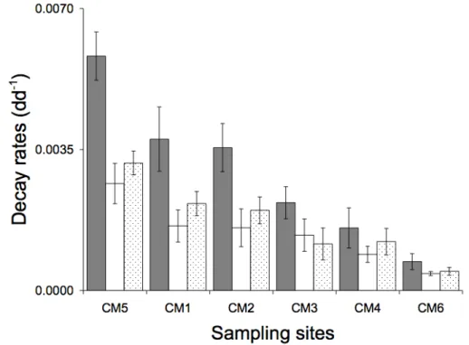
Table 4.2 - Decay rates of leaf detritus ...68 

Table 4.3 - Number of sampled taxa and eigenvector centrality scores. ...70 

Table 4.4 - Correlation between network centralization C(N), the environmental variability given by the coefficient of variation of salinity (CVs), the variation of macrodetritivores activity (CVm) and the number of sampled taxa (S). ...71 

Table 5.1 - Network parameters for each identified taxon...82 

Table 5.2 - Small-world parameters...83 

Table 6.1 - Incidence matrix ...94 

Table A3 1 – Matrix 1 ...132 Table A3 2 - Matrix 2...132 Table A3 3 – Matrix 3 ...132 Table A3 4 – Matrix 4 ...132 Table A3 5 – Matrix 5 ...133 Table A3 6 – Matrix 6 ...133

LIST OF FIGURES

Figure 2.1 – Example of network with 10 nodes and 26 edges. ...22 

Figure 2.2 – A bipartite graph ...25 

Figure 2.3 – Histogram of degree distribution. ...31 

Figure 2.4 – Nestedness matrix ...41 

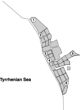
Figure 3.1 – Location of sampling sites in the Biological Reserve of Tarquinia saltern. ...47 

Figure 3.2 – Diversity profiles for sampled pools...51 

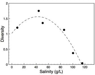
Figure 3.3 – Diversity vs. salinity relationship...52 

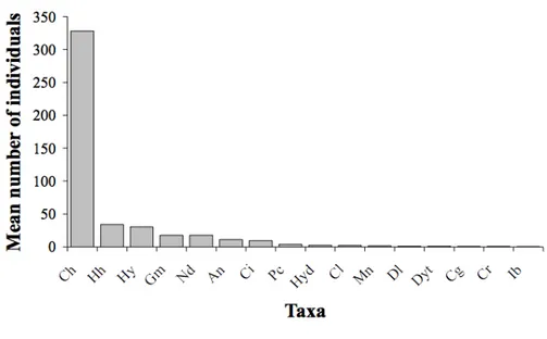
Figure 3.4 – Mean number of individuals vs. observed taxa...53 

Figure 3.5 – Rarefaction curves of species richness. ...54 

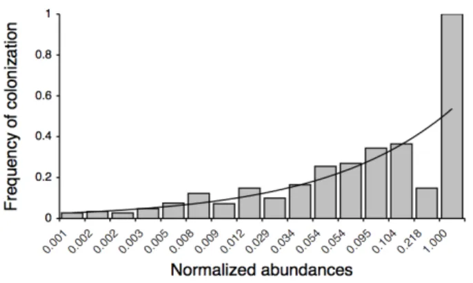
Figure 3.6 – Distribution of the frequencies of colonization and abundances of sampled taxa...54 

Figure 3.7 – Decomposition rates of P. australis leaf detritus...55 

Figure 3.8 – Linear regression between decomposition rates and salinity...56 

Figure 4.1- Box plots showing dry mass remaining (%) of Phragmites australis leaf detritus in coarse and fine mesh bags...68 

Figure 4.2 - Radial visualization of eigenvector centrality. ...71 

Figure 5.1 - A bipartite and unipartite projection of the spatial network of Tarquinia saltern ...81 

Figure 5.2 - k-core partition and closeness centrality...82 

Figure 5.3 - Relationships among centrality values and normalized abundances and frequencies of colonization of macroinvertebrates on leaf detritus ...84 

Figure 6.1 - Spatial location of sampled pools in the Biological Reserve of Tarquinia saltern...93 

Figure 6.2 - Frequency distribution of the mean number of individuals per taxa and relationship between abundances and frequencies of colonization...97 

Figure 6.3 - Modular structure... ...102

Figure 6.4 - Modular matrix...100 

LIST OF PAPERS

A slightly modified version of Chapter 4 has been published on Atti dei Convegni Lincei, Accademia dei Lincei - Cerfolli F, Novelli C, Bellisario B, Nascetti G (2009) Il ruolo del

detrito vegetale autoctono ed alloctono quale regolatore della struttura della comunità macroinvertebrata nell’ecosistema acquatico artificiale delle Saline di Tarquinia. Atti

dei Convegni Lincei 250 - Accademia dei Lincei, Roma (28-03.2008): Acque interne in Italia: Uomo e Natura, pp 99-112.

A slightly modified version of Chapter 5 has been accepted for publication on

Transitional Waters Bullettin e-ISSN: 1825-229X, a international journal edited by the

University of Salento (LE) - Bellisario B, Cerfolli F, Nascetti G (2010)

Macroinvertebrates assembly in a patchy environment: centrality measures for the spatial network of detritus-based communities

A slightly modified version of Chapter 6 has been accepted for publication on Ecological

Research, the official English-language journal of the Ecological Society of Japan, ISSN:

0912-3814 (print version) ISSN: 1440-1703 (electronic version). Journal no. 11284 of Springer Japan. Bellisario B, Cerfolli F, Nascetti G (2010) Spatial network structure and

robustness of detritus-based communities in a patchy environment - IF (2008): 1.206, Journal Citation Reports®, Thomson Reuters

TALKS

Bruno Bellisario, Fulvio Cerfolli, Giuseppe Nascetti - Leaf detritus colonization in a

patchy environment: the spatial structure of detritus-based communities in Tarquinia saltern – 3rd _{Italian Conference on Lagoon research – LAGUNET - Orbetello (GR, Italy)}

1-3 Ottobre, 2009

Bruno Bellisario - Centralization measures of donor – controlled communities on P.

australis leaf detritus in Tarquinia Saltern – Annual Meeting of Italian PhD Student in

Ecology, Parma, Italy, 2009

Bruno Bellisario, Fulvio Cerfolli, Claudia Novelli, Giuseppe Nascetti -

Macroinvertebrates colonization process of Phragmites australis leaf detritus in Tarquinia saltern – 2nd _{Italian Conference on Lagoon research – LAGUNET - Tarquinia}

(VT, Italy) 23-25 Ottobre, 2008

Fulvio Cerfolli, Claudia Novelli, Bruno Bellisario, Giuseppe Nascetti - Donor control

model in the transition ecosystem of Tarquinia salterns: the functional role of bottom up pressures – 3rd _{European Conference on Lagoon Research – LAGUNET – Napoli (NA,}

INTRODUCTION

T

Natural and human induced alterations in space and time have sparked widespread changes in the global distribution of biota, and this results in the expansion of allochtonous, non-native species and contractions of autochthonous, native species, the so-called "biotic homogenization". Homogenization is not a random process, because invasion success and extirpation vulnerability are defined by the interaction between species traits and environmental conditions [107].

Therefore, since species contribute individually and collectively to the stability of communities and ecosystems, the modification of community structure could lead to a structural and functional homogenization, involving the replacement of ecological specialists by the same widespread generalists [134]. Homogenization of communities might also reduce ecosystem functioning, stability and resistance to environmental change by restricting the available range of species-specific responses [164].

The structural composition of communities defines the range of functional traits that influence ecosystem functions (such as the decomposition of organic matter [120]), and the homogenization might limit the pool of species that can compensate for local extinctions (i.e., reduce spatial patterns in functional redundancy). Homogenized communities might therefore have a decreased resistance to environmental perturbations, as the high degree of similarity among communities might dampen or eliminate potential recolonizations by species with locally extirpated traits.

In this work, I wanted to assess the consequences for ecosystem structure and functioning of changing environmental conditions over space and time. Since the effects of biotic homogenization might be particularly high in areas, such as small and fragmented ecosystems that experience more frequent and severe disturbance events, the Biological Reserve of Tarquinia saltern represents a suitable candidate to test hypotheses about functional ecology [26].

The aim of this work is to understand how the steepest gradients of environmental conditions influence the structure and functioning of detritus-based communities. The importance in the study of decomposition processes and dynamics lies in the ability of detritus to sustain higher species diversity, larger predator biomass, and longer food chains than would be supported by primary productivity alone [60], stabilizing the dynamics of consumer populations and food webs that would be otherwise unstable (for a complete review see [120]).

The experimental approach carried out for this work comes from a twelve months field experiment under non-manipulative conditions in six sites in the area of Tarquinia saltern, to cover the full spectrum of environmental gradients, using the allochtonous leaf detritus of Phragmites australis (Cav.) Trin. ex Steud. The

choice of use the allochtonous detrital resource of P. australis comes from its wide spatial distribution, able to be colonized from a variety of organisms, independently from their life history and phenology (e.g., marine and/or freshwater).

Here I applied the network analysis to understand how the whole community assembly and the spatial distribution of macroinvertebrates on leaf detritus are influenced by the environmental conditions under which they are structured, and the consequence for ecosystem functionality and stability.

In this work I also evaluated the role of the spatial assembly of the pools in Tarquinia saltern on the colonization process of leaf detritus. Spatial patterns could affect any of the many processes in communities, such as decomposition [185], spatial subsidies and food-web dynamics, and thereby have cascading effects elsewhere on the landscape. Moreover, an increased spatial similarity in the species identity could have direct and indirect effects on species at lower and higher trophic levels by increasing extirpation rates via intensified species-specific interactions (e.g., functionally similar species might utilize the same resources increasing competition and decreasing functionality), giving useful insights for conservation and management.

This work is divided in two main sections. The first section gives the background in the ecology of detritus-based systems (Chapter 1) and in the framework of complex networks (Chapter 2). The second section represents the core of my work, describing the raw results about the field experiment (Chapter 3), the more fine analyses about the role of salinity on driving the structuring process of communities and the consequences for decomposition (Chapter 4), and the influence of spatial structure on the robustness of ecological communities (Chapters 5 and 6). After the references, the reader can find a series of appendices describing the most used concept in functional and network ecology (Appendix 1), the derivation of the equations used to measure the potential interferences among taxa in the detritus-based communities (Appendix 2), the interaction matrices derived for each community (Appendix 3), and the codes written in R [154] to measure the network parameters and statistics (Appendix 4).

I

PART

The ecology of detritus-based

systems

1.

This chapter gives the background in the ecology of detritus-based systems. Detritus represent a source of energy for many organisms and is able to sustain higher species diversity and longer food chain than would be expected by primary production alone. Environmental conditions influence the decomposition dynamic in aquatic ecosystem via direct and indirect effects, influencing the rate at which detritus is leached by water and conditioned by microfungi and bacteria, and influencing the colonization process by macroinvertebrates, in terms of species diversity and abundance, both of detritivores and their predators. This chapter aims to introduce my work following one main question about the role of the structural patterns of detritus-based communities and their influence on the degree of system functionality, under variable environmental conditions in time and space.

1.1 Introduction

Traditional approaches in ecology emphasize the transfer of local primary productivity through trophic levels. However, detritus is a common feature in most of ecosystems and plays an often-overlooked role of a dynamic heterogeneous resource and habitat for many species. The importance of detritus comes from the ability to regulate the regeneration of carbon and nutrients, being an important link between primary and secondary production [42]. Indeed, most primary production is not consumed by herbivores, but is returned to the environment as detritus, to play a critical role in organizing and sustaining ecosystems [200] [60] [151]. Detritus also physically alters habitats [169] [207], facilitating some species and inhibiting others [64].

Therefore, the importance of decomposition (especially in aquatic ecosystems) comes from the ability to sustain higher species diversity, larger predator biomass, and longer food chains than would be supported by primary productivity alone [60]. Decomposition can also stabilize the dynamics of consumers populations, alter habitat complexity, and stabilize food webs that would be otherwise unstable [120].

This chapter aims to introduce a fundamental question in the study of detritus-based systems: what are the structural patterns that influence the degree of ecosystem functionality under variable environmental conditions in time and space? To answer this question it is necessary to introduce some fundamental concepts in the study of these systems, in order to better understand the role of detritus within ecosystems.

1.2 Definition of detritus

Detritus can be defined as any form of non-living organic matter, including different types of plant tissue (e.g., leaf litter, dead wood, aquatic macrophytes), animal tissue, dead microbes, faeces, as well as products secreted, excreted or exuded from organisms (e.g., extra-cellular polymers).

In the studies of decomposition dynamic in aquatic ecosystems, detritus can be subdivided on the basis of its dimensional classification [32]:

1. DOM: Dissolved organic matter, with a diameter less than 0.5 µm, deriving from soluble organic matter

2. FPOM: Fine particulate organic matter, with a diameter ranging between 0.5 µm and 1 mm, deriving from leaf fragment

3. CPOM: Coarse particulate organic matter, with a diameter up to 1 mm, deriving from leaf, flower and wood

This classification follows a particular dynamic, in which the fractions are in dynamic equilibrium following the order

€

CPOM →FPOM →DOM.

However, this nomenclature derived from the size classification of detritus is far from be standardized. For example, aquatic ecologists usually subdivide particulate detritus into large particles (coarse POM) and small particles (fine POM). In terrestrial ecosystems, where it is difficult to separate aged detritus from the soil matrix, the density distinguishes more labile (the so-called “light fraction” or LF) from the less degradable POM fraction that is incorporated into aggregates, association with clay and silt, and chemical/biological transformation into recalcitrant molecules [176]. The chemical quality of detritus and its decomposition products, combined with physical mixing by organisms, influence nutrient availability, soil chemistry, and soil architecture that, in turn, influence species diversity [22]. Indeed, detritus, other than a source of energy, serves as a habitat and habitat modifier for a variety of organisms.

As highlighted by several authors, both in terrestrial [179] [77] [16] and in aquatic ecosystems [168] [206], detritus modifies the physical structure and conditions of habitats, such as soil moisture, light, temperature, and flow velocity

of wind and water. The turbidity of many estuaries, reservoirs, large rivers, and lakes comes from the high concentrations of detritus, where the attenuation of the light by particulate detritus suspended in water column may reduce the photosynthetic rates and the feeding efficiencies of visually oriented predators [160].

The origin of dead organic matter is often particular, observing how in some ecosystems (e.g., floodplain), a great amounts of detritus, nutrients, and sediments rich in organics are exchanged reciprocally between the river channel and the riparian land via flooding. Allochtonous detritus among habitats is ubiquitous in diverse biomes and is often a central feature of population, consumer-resource, food web and community dynamics, representing a substantial source of energy for many ecosystems.

Indeed, one of the most biomass-rich community on earth is supported entirely by allochtonous detritus, where 15–300 m mats of detrital surfgrass and kelp are converted into 1 kg/m3 of benthic crustaceans (up to 36 individuals/m3), and a large numbers of trophically distinct fish feed in these hotspots [195] (but see [113] for many other examples).

This supports the need to understand the mechanisms that regulate the spatial dynamics of detritus, nutrients, consumers and prey, because ecosystems dynamics are rarely confined within a focal area and that factors outside a system may substantially affect (and even dominate) local patterns, dynamics and stability.

1.3 The decomposition of detritus

Decomposition dynamic in aquatic ecosystems involves three main mechanisms: i) the rapid weight loss of leaf soluble constituents, ii) the modification of leaf matrix by microorganisms and iii) the feeding activity of macroinvertebrates.

Detritus begins to lose soluble organic and inorganic materials shortly after immersion in water. The general pattern of leaching from immersed whole leaves is a rapid loss over the first 24 hours, followed by a gradual decline [119]. It has been found [143] [142] that some variables such as water temperature, turbulence,

salinity and leaf species/quality, influence the decomposition dynamic of leaf detritus.

After leaching, leaves are colonized by a variety of aquatic microbes within a few days of deposition. In general, fungi, principally hypmomycetes, dominate early colonization, gradually giving way to bacteria as decay advances [182]. Aquatic hypmomycetes produce polysaccharide-hydrolyzing exoenzymes including pectinases [181], hemicellulases and cellulases [175], all of which are potentially important in the decomposition of plant material.

However, the structural polysaccharides, cellulose and hemicellulose of plant cell walls are physically and chemically bound to lignin, forming lignocellulose, a resistant complex that renders cellulose and hemicellulose less accessible to enzymes [84], producing a refractory fraction of detritus persisting in the system.

A second mechanism of fragmentation is that promoted by invertebrates. Leaf-shredding invertebrates, or shredders [31], preferentially colonize and feed on microbially conditioned leaves [32] and may contribute significantly to leaf breakdown, especially in aquatic systems.

In ecology, one of the most used models to describe the decomposition dynamic is the negative exponential model, originally developed by Jenny et al. [75] and Olson [136]:

€

W_t = W0e

−kt ₍₁₎

where Wt is the dry weight of leaf detritus at time t, W0 the initial dry weight

of leaf detritus and t the time.

From Eq.1 it is easy to derive the decomposition coefficient, k, expressing the rate at which detritus is decomposed in time t:

€

k =lnWt− lnW0

t (2)

This model has been criticized for two major reasons: first, other mathematical equations often describe the data more precisely, second, variables

known to affect rates of organic matter breakdown, such as temperature, pH and salinity, are not present in the negative exponential model.

The useful of the negative exponential model can be developed from the assumption that the rate of weight loss (or absolute decomposition rate) from organic material is a constant fraction of the amount of remaining material. The major problem encountered in using this model is that breakdown rates are seldom constant.

As noted by Levins [93], there is no single all-purpose model, because models might be built for generality, realism, or precision, but it is not possible to maximize all of these qualities simultaneously. The aim of any model is to maximize realism, such as some of the various modifications of the negative exponential model (see for references [116] [165] [172]), useful for the insight they provide to the mechanisms of breakdown under natural conditions.

Despite these criticisms, the advantage of the exponential model is its generality, because it provides a single number that describes the progress of breakdown in a particular situation, posing the basis for comparing breakdown rates in different situations.

1.4 The detritus-based food webs

Detritus in food webs is a source of energy and nutrients to living organisms. As noticed by Moore and Hunt [123], most of the known food webs available in literature contain both detritus and primary producers. In their work, the authors deconstructed the 40 food webs compiled by Briand [18] into 138 pathways (or energy channels) that originated with a basal resource (i.e., detritus) and ended with a top predator, revealing as many of which could be traced back to detritus.

Food webs normally exhibit a high degree of inter- and intraguild predation and omnivory across the pathways, to the point that a significant amounts of biomass can be traced back to detritus [120]. Some food webs are based almost entirely on detritus [71], as the food webs structured in caves and small stream in forested watersheds, while for others the detritus can have strong influence on the structure and dynamics of grazer pathways [121]. One example is provided by the

reservoirs in the Midwestern USA, where detritivorous fish attain high biomass

via detritus consumption, excreting nutrients that stimulate phytoplankton

biomass [190].

A detritus-based trophic chain in aquatic environment is mainly composed by four elements (also called trophic levels, see Appendix A1). These are the basal level, or the source of dead organic matter, the 1st order consumers (fungi and bacteria), the 2nd order consumers (micro and macrodetritivores, mainly macroinvertebrates) and 3rd order consumers, predators. A constant interlink between the grazer and detritus food chain can be observed by the fact that the 3rd order predators in detritus food web can be a source of food for vertebrates predators of the grazer food web. The complexity of the whole community assemblage may end with the presence of top-predators, those species able to feed at the same time between the grazer and detritus chain.

Detritus has often-important implications for the interpretation of many classic ecological theories, such as the stability of food webs, trophic height or food chain length, the distribution of biomass among trophic levels, trophic cascade and biodiversity (see Appendix A1). The stabilizing effect of detritus is achieved not through self-limitation of the resource (as in classic primary-producer models) but, rather, as a result of the constant inputs of detritus. Indeed, several authors [122] [127] have shown how detritus represents a more stable and persistent reservoir of energy than primary producers alone, over a wide gradient of productivity.

As noticed by many [123] [60] [83] detritus was found to support long food chains. The number of trophic levels is a central issue in the study of food chain dynamics [133] and the structuring of ecosystems via trophic cascades [25], as well as mediating the relationship between species diversity and ecosystem function [209] [37].

One of the earliest explanations for what constrains the number of trophic levels was forwarded by Elton [39]. His productivity hypothesis posited that, due to the inherent inefficiency of trophic transfers, available energy becomes insufficient to support more than a small number of trophic levels. A testable prediction of this hypothesis is that more productive ecosystems should have

longer food chains. Because of the resident time of energy within detrital systems is longer owing to the absence of death, and the internal cycling in detritus-based systems enhances the efficiency of detrital vs. grazer-dominated food webs, this source of energy can support species at higher trophic levels, longer food chains and greater food web complexity [120].

This latter represents one of the fundamental and controversy issue in the study of ecological communities. Early theoretical consideration suggested that the presence of more feeding link (complexity) among more species (diversity) generally reduces the risk of species dependence on a few resources [98].

Starting from the late 1950’s, the notion that complexity begets stability was considered by many ecologists one of the basic ecological theorem [73]. However, the apparent inevitability of this relationship was challenged by mathematical models of food webs dynamic, which showed how diversity and complexity might destabilize ecosystems through increasing the chance of positive feedback [101]. In particular, Pimm and Lawton [149] concluded that long food chains tend to be dynamically fragile, and less able to recover from environmental perturbation. A resulting prediction was that food chains should be shorter in ecosystems subject to environmental fluctuations and disturbances [147]

Thus, understanding the role of complexity (e.g., the number of interactions among species in a community) and diversity (e.g., the number of species in a community) represents a fundamental issue in the face of our understanding of ecosystem function. Which species are important and how they interact to create and maintain species diversity patterns represents a key issue to understand the mechanisms of decomposition processes.

Several authors have shown a significant decrease in the rate of leaf litter decomposition with declining species richness, both in terrestrial [125] and in aquatic ecosystems [200]. However, decomposition may be only weakly correlated with species richness and the total abundance of detritivores organisms, because some species are far more important than others.

This view supports the idea that the presence of keystone taxa (i.e., topological keystone species [80]) may be more important for decomposition

[196] than species diversity per se. Many laboratory and field studies suggest that species richness can be related to the rate at which leaf detritus is broken in stream ecosystems [78], showing a little redundancy among species in their effect on ecosystem process, on the contrary of what observed in marine environment [0], where the functional diversity among species seems to be more correlated whit the decomposition rate. Thus, understanding how the environment constraints the structural pattern of ecological communities will provide a more understanding of our knowledge about functionality, also in the face of environmental change.

Related to the above discussion is the fundamental question of what determines how many species are to be found in a given place and how they interact to maintain ecosystems functioning. One can ask why there are a well-defined number of species co-occurring in a given place and why not more or fewer similar species.

In the late 1961’s, Hutchinson [72] posed the paradox of plankton, noticing how phytoplankton communities generally exhibit high species number despite apparent limited opportunities for niche partitioning of their resource. Niche differentiation is obviously an important aspect, however, it is clear that other mechanisms must be involved, as similarity in coexisting species. High diversity of coexisting species can results from spatial heterogeneity [186], temporal variability [92], spatial structure and interactions between competition and colonization [48], and trophic complexity [139]. In addition, high diversity of competitors could result from the interplay of speciation and extinction process in systems in which all competing species were functionally identical (the so called neutral theory of biodiversity [70]).

The question early posed by Hutchinson and MacArthur reaches answers in the intuition of many naturalists that niches of all of seemingly similar species really differ in aspects that are not easily detected [166]. Another, slightly less intuitive, class of explanations for the coexistence of so many species in nature is that various mechanisms may help to prevent competitive exclusion. As noticed, these mechanisms might be predation [139], chaotic population dynamics [167], environmental variability [177] [27] and incidental disturbances [28]. The

interaction of such mechanisms at multiple scales of space and time may maintain much of the biodiversity observed in nature [91].

Niche differentiation, or facilitative interactions among species within trophic levels, maximizes ecosystem processes such as productivity [70] or decomposition [178] as diversity increases. Ecological niche differentiation may be correlated with phylogenetic divergence among species, and so indicates the potential for complementarity in function [100].

The role of the mixing pattern of interactions in ecological communities is a fundamental issue to understand species coexistence and to make prediction about ecosystems functioning. Indeed, species interactions are found to be of greater influence on decomposition dynamic, suggesting how the richness-functioning relationship may be driven by direct (abundances) and indirect (predation and competition) mechanisms [35]. Factors such as competition between the organisms involved in detritus decomposition have been suggested to regulate the dynamics between trophic levels [197], and the increased trophic complexity (i.e., the presence of predators) will potentially enhance the consumption rate by detritivores [120].

It has been found how the interlink among uncertainty in environmental conditions, predation and competition in ecological communities may determine relative abundances of species [202]. This regulation in populations and the determination of relative abundances are determined by complex interactions among the life histories of the species, their defenses against predators, and their competitive abilities.

The size-structured interactions among species in community may change connections through seasonal shifts in trophic links. This allow a different way of thinking about food webs, moving away from the static concept of stable linkages among taxa to include some of the spatial and temporal mechanisms that make actual food webs constantly changing tangles of trophic relationships [201]. Thus, the impact of detritus into food webs analyses must be focused not only on the characterization, classification and transformation of detritus, but often on the role that the detritus has for community organization. This is because detritus goes

through a series of changes through time, and these changes are both mediated by and have large effects upon the organisms that process the detritus.

These transformations represent multiple entry points into the system and the infusion of this energy into the community and its passage to top predators affects the diversity, structure and dynamic properties of the community.

II

PART

2

In the past few years, the framework of complex networks has provided new insight into the organization and function of many biological systems, representing a useful tool to describe many physical, biological and social systems. Network theory is now a truly interdisciplinary topic, and ecology has drawn heavily upon algorithms developed in other areas, such as social science and information theory. In this chapter I want to introduce the basic concept in network analysis, and highlight the most used network properties in the study of ecological and spatial networks. After the necessary introduction to the common statistical measures I briefly look inside the network measures I used to analyze data in this work.

2.1 Introduction

A network can be defined as a set of items called vertices or nodes, with connections (called edges) between them (Fig. 2.1).

Figure 2.1 – Example of network with 10 nodes and 26 edges.

In real life, there are many examples of systems taking the form of networks, also called graphs in mathematical literature. Some examples include the Internet, the World Wide Web, social networks of acquaintance or other connections between individuals, organizational networks and networks of business relations between companies, neural networks, metabolic networks, food webs, distribution networks such as blood vessels or postal delivery routes,

networks of citations between papers, and many others.

The study of networks, in the form of mathematical graph theory, is one of the fundamental pillars of discrete mathematics. Recent years, have witnessed a substantial new movement in network research, with the focus shifting away from the analysis of single small graphs and the properties of individual vertices or edges within such graphs to consideration of large-scale statistical properties of graphs. The body of theory in network analysis focuses mainly on three fundamental aspects: i) the statistical properties able to characterize the structure and behavior of networked systems, and to suggest appropriate ways to measure these properties, ii) the models of networks that can help us to understand the meaning of these properties - how they came to be as they are, and how they interact with one another, and iii) what the behavior of networked systems will be on the basis of measured structural properties and the local rules governing individual vertices.

This is because structure affects the functioning of systems and, therefore, a proper understanding of the structural characteristics of the network involves a greater understanding on their functioning.

2.2 Types of networks

In real world, there may be more than one different type of vertex in a network, or more than one different type of edge, and vertices or edges may have a variety of properties, numerical or otherwise, associated with them. The edges of graphs may also be imbued with directedness so, a normal graph in which edges are undirected is said to be undirected.

In the most common sense, a network (or graph) is an ordered pair

€

G := (V, E), comprising a set V of vertices or nodes together with a set E of edges

or lines, which are 2-element subsets of V. Otherwise, if arrows may be placed on one or both endpoints of the edges of a graph to indicate directedness, the graph is said to be directed.

A directed graph in which each edge is given a unique direction (i.e., edges may not be bidirected and point on both directions as once) is called an oriented graph. An undirected graph, is a graph in which edges have no orientation, i.e.,

they are not ordered pairs, but sets {u, v} (or 2-multisets) of vertices. A directed graph (or digraph), is an ordered pair of

€

D := (V, A) , with V as a set whose

elements are called vertices or nodes and A, a set of ordered pairs of vertices called arcs, directed edges or arrows. A directed graph D is called symmetric if, for every arc in D, the corresponding inverted arc also belongs to D. A symmetric loopless directed graph

€

D := (V, A) is equivalent to a simple undirected graph

€

G := (V, E), where the pairs of inverse arcs in A correspond one-to-one with the

edges in E; thus the edges in G are |E| = |A|/2, or half the number of arcs in D. A further essential aspect in network theory is to consider not only the number of connections (edges) among nodes, but also the weight that each connection has. This is the case of a weighted graph, having a numerical label

w(E) associated with each edge E, called the weight of edge. Edge weights can be

integers, rationale numbers, or real numbers, which represent a concept such as distance, connection costs, or affinity.

Mathematically, a network or graph can be expressed in two different ways, a one-mode data matrix and a two-mode data matrix. A one-mode data matrix is the classical representation in which the elements in rows are the same in columns, and each matrix element xij represents the presence/absence (in a binary

0-1 representation) of a relationship among them. Clearly, matrix element can be weighted, expressing a quantitative relationship between i and j.

In ecology, a one-mode matrix depicts a kind of direct relationship among nodes that can be represented as a set of species in a community, typically a food web expressing who eat whom in a community. A two-mode data consist of a data matrix A over two sets U (rows) and V (columns). Such data can be viewed also as a bipartite network, in which links are established between two sets of nodes (U and V) but not within the same set (Fig. 2.2). A 2-mode network is a structure (U, V, R, w), where U and V are disjoint sets of vertices (nodes or units), where

R ⊆ U x V is a relation, and

€

w : R → ℜ is a weight. If no weight is defined we can

assume a constant weight w(U, V) = 1 for all (U, V) ∈ R. A 2-mode network can be viewed also as an ordinary one-mode network on the vertex set U + V, divided into two sets U and V, where the arcs can only go from U to V (a bipartite directed graph).

Figure 2.2 – A bipartite graph in which links are established between two sets of nodes but not

within nodes of the same set.

2.3 Properties of networks

The simplest, useful model of a network is the first studied by Rapoport [155] and Erdós and Rényi [40]. In this model, undirected edges are placed at random between a fixed number n of vertices to create a network in which each of the 1/2(n - 1) possible edges is independently present with some probability p, and the number of edges connected to each vertex - the degree of the vertex - is distributed according to a binomial distribution, or a Poisson distribution in the limit of large n. Real networks are non-random in some revealing ways that suggest both possible mechanisms that could be guiding network formation, and possible ways in which we could exploit network structure to achieve certain aims.

Here I briefly explore some of the basic features in network analysis, referring to Newman [129] for a complete review in network theory.

2.3.1 The small world of real networks

The significance of small world lies in the fact that most pairs of vertices in most networks seem to be connected by a short path through the network, the so-called six-degree of separation, following Milgram's experiment [114], set in a more mathematically rigorous way by Pool and Kochen [152].

Consider an undirected network with l as the mean geodesic (i.e., shortest) distance between vertex pairs in a network with n nodes:

€

l = 1

0.5n(n + 1)

∑

where dij is the (geodesic) distance from vertex i to vertex j.

The quantity l can be measured for a network of n vertices and m edges in time O(mn) using simple breadth-first search, also called a burning algorithm in the physics literature [1]. In Table 1, are shown the values of l takes from the literature for a variety of different networks, in which the values are in all cases much smaller than the number n of vertices, for instance.

Table 2.1 – Shortest paths among different types of networks.

Network Type n l

Film actors Undirected 449913 3.48

Physics coautorship Undirected 52909 6.19

Citation network Directed 783339 5.22

S oc ia l n et w or k

Email messages Directed 59912 4.95

Metabolic network Undirected 715 2.56

Protein interactions Undirected 2115 6.8

Marine food web Directed 135 2.05

Freshwater food web Directed 92 1.9

B io lo gi ca l n et w or k

Neural network Directed 307 3.97

The small-world effect has obvious implications for the dynamics of processes taking place on networks. For example, if one considers the spread of information across a network, the small-world effect implies that spread will be fast on most real-world networks. Networks are said to show the small world effect if the value of l scales logarithmically or slower with network size for fixed mean degree.

2.3.2 Clustering

A fundamental measure that has long received attention in both theoretical and empirical network research is the clustering coefficient, measuring the degree to which nodes tend to cluster together. Evidence suggests that in most real-world networks, nodes tend to create tightly knit groups characterized by a relatively high density of ties [199].

As I previously shown, a graph G = (V, E) consist of a set of vertices V and a set of edges E between them, and an edge eij connecting vertex i with vertex j.

The neighborhood N for a vertex vi is defined as its immediately connected

neighbors as follows:

€

N_i= v

{

}

In this context, I introduce the next statistical properties of the networks, the degree ki of a vertex, defined as the number of vertices,

€

N_i , in its neighborhood

Ni. The local clustering coefficient Ci for a vertex vi is then given by the

proportion of links among the vertices within its neighborhood, divided by the number of links that could possibly exist among them. In a directed graph it is possible to observe two distinct edges, eij ≠ eji, and therefore for each

neighborhood Ni there exist ki (ki - 1) links among vertices.

This means that a generic node i could have an ingoing and an outgoing link (the in- and out-degree). The clustering coefficient for the whole system [199] is defined as: € C = 1 n _i=1Ci n

∑

{

}

and € C_i = 2 e

{

_}

The degree of a vertex is the number of edges incident on (or connected to) that vertex, and it is defined as the fraction pk of vertices in the network that have

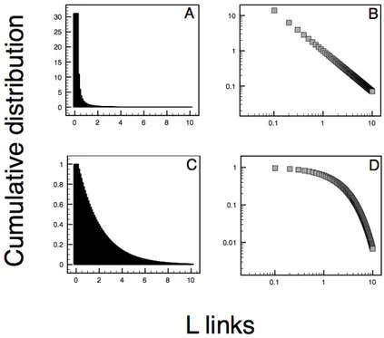
degree k. In network theory, the degree distribution of a vertex could be represented by a filled histogram showing the distribution of the number of links each node has. Clearly, the distribution can be highly skewed, meaning that the distribution has a long tail of values that are far above the mean.

An alternative (and more useful) way of presenting degree data is to make a plot of the cumulative distribution function, expressing the probability that the degree is greater than or equal to k:

€

P_k = p_k,

k,_{= k}

∞

∑

Several studies [199] have shown how real life network may follow an exponential degree distribution,

€

P(≥ Li) ∝ exp(−γL), which indicates that nodes inside the network have a well-defined average number of links. Some others follow a power-law distribution [3],

€

P(≥ Li) ∝ L

−γ_{, characterized by the}

asymmetry in the frequency distribution of link per node, where the bulk of nodes have a few links and a few nodes are much more connected than expected by chance. Some networks have found to follow a truncated power-law,

€

P(≥ L_i) ∝ L−γ_{exp(−L /L}

x) where, at some critical level of connections (Lx), it can be observed a change in network topology, from a typical scale-free distribution to a single-scale distribution with a faster exponentially decay.

The rationale for the importance in degree distribution lies behind the fact that it affects the robustness to node deletion [3] and, thus, the stability of the network.

2.3.4 Centrality

Centrality is one of the most studied concepts in social network analysis. Numerous measures have been developed, including degree centrality, closeness, betweenness, eigenvector centrality, information centrality, flow betweenness, the rush index, the influence measures. What is not often recognized is that the formulas for these different measures make implicit assumptions about the manner in which things flow in a network.

For example, some measures, such as Freeman’s closeness and betweenness [47], count only geodesic paths, apparently assuming that whatever flows through the network moves only along the shortest possible paths. Other measures, such as flow betweenness [46], do not assume shortest paths, but do assume proper paths in which no node is visited more than once. Still other measures, such as Bonacich’s eigenvector centrality [15] and Katz’s influence [82], count walks, which assume that trajectories can not only be circuitous, but also revisit nodes and lines multiple times along the way.

Regardless of trajectory, some measures (e.g., betweenness) assume that what flows from node to node are indivisible (like a package) and must take one path or another, whereas other measures (e.g., eigenvector) assume multiple paths simultaneously (like information or infections).

Here I discuss the eigenvector centrality because this measure is defined in a way that a node centrality depends not only on the topological characteristic of nodes (e.g., the number of connections), but also on their weight (e.g., some properties of interaction strength) (but see Chapter 5 for discussion about other measures of centrality). Eigenvector centrality is defined as the principal eigenvector of the adjacency matrix defining the network.

The defining equation of an eigenvector is:

€

where A is the adjacency matrix of the graph, λ is a constant (the eigenvalue), and

€



x is the eigenvector.

The equation lends itself to the interpretation that a node that has a high eigenvector score is one that is adjacent to nodes that have themselves high scorers. The idea is that even if a node influences just one other node, which subsequently influences many other nodes (who themselves influence still more others), then the first node in that chain is highly influential.

It can be shown [15] that an eigenvector is proportional to the row sums of a matrix S formed by summing all powers of the adjacency matrix, weighted by corresponding powers of the reciprocal of the eigenvalue:

€

S = A +λ−1A2

+λ−2A3

+ ..λ−nAn +1 ₍₁₀₎ It is also well known that the cells of the matrix powers give the number of walks of length k from node i to node j. Thus, the measure counts the number of walks of all lengths, weighted inversely by length, which emanate from a node. Eigenvector centrality is consistent with a mechanism in which each node affects all of its neighbors simultaneously, as in a parallel duplication process hence, is ideally suited for influence type processes.

2.3.5 The resilience of networks

Related to degree distributions is the property of resilience of networks to the removal of their vertices.

If vertices are removed from a network, pairs will become disconnected and any kind of communication between them through the network will become impossible. There are also varieties of different ways in which vertices can be removed, and different networks show varying degrees of resilience to these. One could remove vertices at random from a network, or one could target some specific vertex, such as those with the highest degree.

The consequence of node removal on network resilience is related to the

shape of the links distribution in the network (Fig. 2.3).

By definition, a power-law distribution shows a much more robustness against random removal of nodes, but high sensitivity to the removal of most

connected nodes, as showed in [4]. This is because bulks of nodes have a few links, and a few nodes are much more connected than expected by chance so, the probability to disconnect the system with a random attack is very small. On the contrary, a less skewed distribution reveals a much more sensitivity to random removal of nodes and, thus, on network resilience. Following these studies, many authors have looked into the question of resilience for other networks, observing how most networks are robust against random vertex removal but considerably less robust to targeted removal of the highest-degree vertices (as in metabolic networks [76], or food webs [38]).

Figure 2.3 – Histogram of degree distribution. On the left, the histogram for a power (A) and

exponential distribution (C). On the right, the same distribution expressed as the cumulative degree distribution in a log-log graph of P (y-axis) and the number of links L (x-axis) for a power (B), and exponential distribution (D). The power-law has a much more skewed distribution than an exponential. In a log-log graph, a straight line expresses a power-law.

2.4 Networks in ecology

The origins of networks in ecology date back to the early years of graph theory [65], developed by receiving input from economical network analysis [62] and sociometry [66].

An ecological network is the representation of the biotic interactions in a given ecosystem, in which species (nodes) are connected by pairwise interactions (links). These interactions can be trophic (predator/prey), non trophic (competition, apparent competition) or mutualistic (as in plant-pollinator network). Historically, research into ecological networks developed from descriptions of trophic relationships in aquatic food webs. However, recent works have expanded to look at other food webs as well as webs of mutualists, identifying several important properties of ecological networks.

In this section I show some of the fundamental structural measures in ecological network analysis, shown in more detail in the next section:

1. Connectance: the proportion of possible links among species that are realized. In food webs, the level of connectance is related to the statistical distribution of links per species.

2. Clustering: the proportion of species that are directly linked to a focal species. A focal species in the middle of a cluster may be a keystone species, and its loss could have large effects on the network.

3. Compartmentalization: the division of the network into relatively independent sub-networks. Compartmentalization can be related to body size [170] [158], spatial location [86] or temporal niche availability [96].

4. Nestedness: the degree to which species with few links have a sub-set of the links of other species, rather than a different sub-set of links. In highly nested networks, guilds of species that share an ecological niche contain both generalists (species with many links) and specialists (species with few links, all shared with the generalists).

Given the network-like quality of many ecological phenomena, network analysis may be ideally suited for understanding ecological systems. For example, it may help to identify the processes by which species are able to coexist in communities [33].

However, the use of graph-theoretic approaches by ecologists is limited to a few specific contexts, and most ecological studies involving graph-theoretic approaches focus on the structure of food webs [19] [145] [203], with occasional forays into landscape ecology [189] and nearest-neighbor analysis in plant ecology [34].

The relationship between ecosystem complexity and stability is one of the major topics of interest in ecology, and the use of ecological networks makes it possible to analyze the effects of network properties on the stability of ecosystems (see Appendix A1). Ecosystems complexity was once thought to reduce stability by enabling the effects of disturbances, such as species loss or species invasion, to spread and amplify through the network.

However, other characteristics of networks structure have been identified to reduce the spread of indirect effects and, thus, enhance ecosystem stability. Interaction strength may decrease with the number of links among species, damping the effects of any disturbance [192], and cascading extinctions are less likely in compartmentalized networks as effects of species losses are limited to the original compartment [86].

The community of species in ecosystem is expected to affect both the ecological interactions and coevolution of pairs of species. Related, spatial applications are being developed for studying metapopulations, epidemiology, and the evolution of cooperation. In these cases, networks of habitat patches (metapopulations) or individuals (epidemiology, social behavior) make it possible to explore the effects of spatial heterogeneity. Furthermore, as long as the most connected species are unlikely to go extinct, several studies have shown as stability increases with complexity (e.g., connectance in [38], and nestedness in [23]).

2.4.1 Connectance

Connectedness is a general term describing the degree to which components of a system are connected to each other [5]. Its application in ecology focuses on interactions resulting in energy transfers and food webs. Martinez [103] assessed different aspects of connectedness from the ecological literature, and showed that connectance, and particularly directed connectance, was the most robust measure under different resolutions of food web data.

Mathematically, connectance refers to the ratio of the observed links (L) on the maximum possible number of feasible links in the system (S2) [49]:

€

C = L

S2 (11)

Eq.11 measures the direct connectance, where the denominator expresses all the possible links in an S x S matrix, including self-connectance or cannibalism. Connectance can be also expressed as the interactive connectance, where the denominator is given by S(S - 1), ignoring or disallowing self-connectance or cannibalism.

As any structural properties in network analysis, also the connectance implies a minimum value for any web of S species that can be estimated from the minimum number of links, Lmin, required to interlink species into a single web [50]. This is because a connectance of zero is a contradiction in terms, because network with a connectedness of zero (e.g., a food web) is not a web.

In a network, or food web of S species, the minimum number of possible links is clearly S - 1 so, it is possible to rewrite the Eq.11 as:

€

C_MIN=(S −1)

S2 (12)

The denominator can take any value from the type of connectance you want to measure. Normalizing Eq.12 it is possible to derive a measure of connectance with no bias for network size:

€

CN=

C − CMIN

1− CMIN

(13) The set of equations 11, 12 and 13 expresses the way in which connectance can be measured in a one-mode matrix, or S x S matrix.

For a two-mode matrix, and thus for a bipartite web in which links are established between two different set of nodes (a and b), but not among nodes of the same set, connectance (Cb) must be expressed as the number of observed links

(L) divided by all the possible links: Cb = L / ab.

2.4.2 Clustering

Aggregations of biological species on the basis of trophic similarity (namely trophospecies, see Appendix A1) are the basic units of study ecological networks as food webs, but little attention has been devoted to articulating objective protocols for defining such aggregations [211]. Quantitative patterns in food webs have been the subject of the controversy for several years [103]. The clustering of species on the basis of their trophic similarity helps ecologists to investigate resolution-related issues with statistics commonly used to describe the patterns. To cluster species in the raw food web, the nodes are hierarchically clustered based on the amount of trophic overlap among taxa [103].

In deciding whether two trophospecies should be assigned a trophic link, the maximum linkage convention (in which a link is included if any pair of original trophic entities are linked) produced more aggregation than the minimum linkage convention (in which a link is included only if every pair of original trophic entities is linked).

A one usually way to measure clustering among species is the trophic overlap given by the similarity index (I), calculated using the algorithm defined by Jaccard [74]:

€

I = c /(a + b + c) (14)

where c = number of predators and prey common to the two nodes,

predators and prey unique to the other node. When two nodes have the same set of predators and prey, I = 1, and when two nodes have no common predators or common prey, I = 0.

However, as highlighted in the work of Yodzis and Winemiller [211]: ‘[The] choice of similarity level for defining trophospecies remained an

unresolved issue based on our analysis of our dataset. Perhaps, the greatest challenge is posed by sampling bias within empirical datasets, and we ultimately conclude that it is difficult to identify trophospecies [..] by strictly objective criteria’.

A fundamental contribution may result from the use of modern isotopic techniques [153], used to trace the migration of organisms and the flow of water and nutrients through organisms and ecosystems. They can be used to reconstruct the diet and trophic position of animals, evaluate trophic structure of entire ecosystems and explore niche differentiation among individuals, populations, and communities.

2.4.3 Compartmentalization

Compartments are subgroups of nodes in which many strong interactions occur within the subgroups and few weak interactions occur between the subgroups, increasing the stability of networks. In social sciences, cohesive subgroups in human communities have been an important concept since the 1950’s, when it was proposed that social systems were more efficient and durable when composed of subgroups in which interactions were concentrated [174].

As showed by several authors [101] [147], the structure of food webs is an important property for understanding their dynamic and topological stability. Food web structure was represented in many studies composed by guilds [162], blocks and modules [101], cliques and dominant cliques [212], compartments [147] and sub-webs [138]. Current studies show that groups of species are more connected internally than they are with other groups of species [118], showing how the weak links connecting these subgroups of nodes are the glue that maintains systems stability [105].

An interesting measure in network compartmentalization is given by its modularity. The importance of modularity has been discussed for a long time, but no consensus on its prevalence in ecological networks has yet been reached, because progress in modularity analysis has been hampered by inadequate methods and a lack of large ecological datasets [135]. One main critique in finding compartments (also defined "communities" or modules in the physical literature) in networks is given by the assumption that with hierarchical clustering methods (e.g., Eq.14) one needs to decide where to cut in order to obtain the relevant modules.

Recent development in statistical mechanics showed how it is possible to find modules (also called communities) in a variety of ecological (e.g., food webs, plant-animal mutualistic webs) and non-ecological (e.g., spatial webs) networks, assuming that the network of interest divides naturally into subgroups, whose number and size are determined by the network itself. One of the central algorithm used to find modules in networks, explicitly admits the possibility that no good division of network can exists a priori.

This algorithm is based on a process derived from the physical process of simulated annealing (SA), using a heuristic procedure to find an optimal solution [85]. The name and inspiration come from annealing in metallurgy, a technique involving heating and controlled cooling of a material to increase the size of its crystals and reduce their defects. The heat causes the atoms to become unstuck from their initial positions (a local minimum of the internal energy) and wander randomly through states of higher energy; the slow cooling gives them more chances of finding configurations with lower internal energy than the initial one.

In analogy, each step of the SA algorithm replaces the current solution by a random approximated solution, with a probability that depends on the difference between the corresponding function values and on a global parameter T (defined “temperature”), gradually decreased during the process.

Among the many algorithms implemented to detect community structure in networks during the last few years [131] [58] [57], is of great interest the one developed by [157], implemented in the igraph package of R [154]. The community structure of the network is interpreted as the spin configuration that