R E S E A R C H
Open Access
Do green spaces affect the spatiotemporal
changes of PM
2.5
in Nanjing?
Jiquan Chen
1,2,6*, Liuyan Zhu
1, Peilei Fan
3,2, Li Tian
4and Raffaele Lafortezza
5,2Abstract
Introduction: Among the most dangerous pollutants is PM2.5, which can directly pass through human lungs and
move into the blood system. The use of nature-based solutions, such as increased vegetation cover in an urban landscape, is one of the possible solutions for reducing PM2.5concentration. Our study objective was to understand the importance of green spaces in pollution reduction.
Methods: Daily PM2.5concentrations were manually collected at nine monitoring stations in Nanjing over a 534-day period from the air quality report of the China National Environmental Monitoring Center (CNEMC) to quantify the spatiotemporal change of PM2.5concentration and its empirical relationship with vegetation and landscape structure in Nanjing.
Results: The daily average, minimum, and maximum PM2.5concentrations from the nine stations were 74.0, 14.2,
and 332.0μg m−3, respectively. Out of the 534 days, the days recorded as“excellent” and “good” conditions were found mostly in the spring (30.7 %), autumn (25.6 %), and summer (24.5 %), with only 19.2 % of the days in the winter. High PM2.5concentrations exceeding the safe standards of the CNEMC were recorded predominately during the winter (39.3–100.0 %). Our hypothesis that green vegetation had the potential to reduce PM2.5concentration was accepted at specific seasons and scales. The PM2.5concentration appeared very highly correlated (R2> 0.85) with green cover in spring at 1–2 km scales, highly correlated (R2> 0.6) in autumn and winter at 4 km scale, and moderately correlated in summer (R2> 0.4) at 2-, 5-, and 6-km scales. However, a non-significant correlation between green cover and PM2.5concentration was found when its level was >75μg m−3. Across the Nanjing urban landscape, the east and southwest parts had high pollution levels.
Conclusions: Although the empirical models seemed significant for spring only, one should not devalue the importance of green vegetation in other seasons because the regulations are often complicated by vegetation, meteorological conditions, and human activities.
Keywords: PM2.5, Green space, Edge density, Nanjing, Pollution control, Seasonal variation, Nature-Based Solution (NBS) Introduction
Smog, also known as “smoke fog” (i.e., combination of smoke and other atmospheric pollutants), has become increasingly recognized as a primary environmental problem in many cities worldwide. The problem spread widely in European and North American cities in the 1950s and 1960s but has since become more pro-nounced in developing countries (e.g., India, China) (Rohde and Muller 2015; Zhang and Cao 2015). Among
the most dangerous pollutants is particulate matter of 2.5 μm or less in diameter—PM2.5—as it can pass dir-ectly through human lungs and into the blood system. It is notorious for its role in increasing heart disease, stroke, emphysema, and lung cancer (Apte et al. 2015; Tong et al. 2015).
PM2.5 concentration is primarily determined by the emission source within an urban landscape and its area of reach (Querol et al. 2004; Rohde and Muller 2015). Heavy industries and the escalating number of vehicles, fugitive dust, and biomass combustions are the main causes of high pollutants throughout global cities (Rodrıguez et al. 2004; Giugliano et al. 2005; Park and Kim 2005;
* Correspondence:[email protected]
1International Center for Ecology, Meteorology, and Environment, Nanjing University of Information Science and Technology, Nanjing 210044, China 2CGCEO/Geography, Michigan State University, East Lansing, MI 48824, USA Full list of author information is available at the end of the article
© 2016 Chen et al. Open Access This article is distributed under the terms of the Creative Commons Attribution 4.0 International License (http://creativecommons.org/licenses/by/4.0/), which permits unrestricted use, distribution, and reproduction in any medium, provided you give appropriate credit to the original author(s) and the source, provide a link to the Creative Commons license, and indicate if changes were made.
Viana et al. 2008; Mugica et al. 2009; Perrone et al. 2012). Atmospheric conditions such as vertical and horizontal temperature, atmosphere pressure, wind speed, and water vapor density are mostly responsible for PM2.5 dispersion (i.e., the sinks) (Liu 1985; Janhäll 2015; Rohde and Muller 2015). Consequently, the temporal changes in local and regional climate play
fundamental roles in PM2.5 concentrations over
hourly to interannual time scales (Hueglin et al. 2005; Vecchi et al. 2007), leading to high levels during the night (Vecchi et al. 2007) and in winter (Vecchi et al. 2004; Giugliano et al. 2005; Zhang and Cao 2015). Within the landscape, PM2.5 can be decomposed over time through multiple chemical, physical, and bio-logical processes such as dry and wet deposition. Land surface properties, such as roads, construction, and vegetation, can directly filter pollutants and indir-ectly influence the air movement through its hetero-geneous urban canopies (Janhäll 2015). While the ultimate solution for most cities is to eliminate the
emission sources, other proposals to reduce PM2.5
concentration are also underway; these include engin-eering methods for filtration and uptake (Hänninen et al. 2005) or using nature-based solutions (NBS), such as increasing vegetation cover in urban landscapes.
Over the years, one of the most favored NBS to deal with urban problems, such as pollution reduction, has been to increase green vegetation. It has been theorized that green vegetation has the potential to reduce pollut-ants through filtration (Hwang et al. 2011) and the abil-ity to regulate microclimatic conditions (Chen et al. 1999; Lafortezza et al. 2009). In a recent meta-analysis of 102 peer-reviewed publications on urban green space, urban heat islands, and air quality, Zupancic et al. (2015) stated that,“In general, the research suggests that balan-cing urban forest density, particularly in areas with low green space density, would greatly improve both local-and city-wide urban air quality.” The empirical local-and mechanistic functions of green spaces in reducing PM2.5 and other pollutants have also been reported in an in-creasing number of studies over recent decades. Based on a controlled experiment, Hwang et al. (2011) found that coniferous trees are more effective in filtering small particulates than broadleaf trees. Chen et al. (2015) dem-onstrated that PM2.5 inside forest shelterbelts is signifi-cantly higher than outside (i.e., captured pollutants), especially for larger particulates (e.g., PM10). At land-scape level, Wu et al. (2015) found that the total vegeta-tion cover and its spatial configuravegeta-tion (e.g., edge density, patch density, and aggregation) in Beijing could reduce annual PM2.5 concentration. Altogether, the roadside vegetation was credited for removing 1.09 Mg PM2.5 per year in Beijing (Tong et al. 2015). In the United States, Nowak et al. (2013) reported that, “The total amount of
PM2.5removed annually by trees varied from 4.7 t in Syra-cuse to 64.5 t in Atlanta, with annual values [of the trees in pollution reduction] varying from $1.1 million in Syra-cuse to $60.1 million in New York City.”
The PM2.5 concentration in an urban landscape is not static, but varies greatly in time and space (Querol et al. 2004; Nowak et al. 2013; Janhäll 2015) because of the dynamic meteorological conditions, heterogeneous land surface properties, uneven distribution of emission sources, landforms, and other human activities (e.g., ve-hicle use and biomass burning). Regardless of the large number of studies on vegetation and PM2.5 concentra-tion, it is unclear if the role of vegetation in reducing PM2.5 concentration remains the same in different sea-sons and under varying pollution levels. This is espe-cially critical for the cities in temperate zones where vegetation structure (e.g., amount and types of leaves) and composition (e.g., evergreen vs deciduous) are dis-tinctively different among the four seasons. One would logically reason that the role of vegetation in filtering pollutants would be stronger with an elevated leaf sur-face, a higher leaf quantity, a more complex vertical can-opy structure, a higher edge density, and numerously dispersed patch patterns (Janhäll 2015). These stand and landscape characteristics would raise a higher surface in three-dimensional space to capture more pollutants and would also promote a higher vapor density (Chen et al. 1999), which has the potential to reduce dust while in-creasing wet deposition. While some of these features do not change (e.g., land form), vegetation structure is highly dynamic, suggesting that the reduction will be highly dependent on seasons. Finally, the effect of a spe-cific location in the landscape on PM2.5 depends on the surrounding vegetation (amount and configuration). Yet, we do not know the effective footprint of vegetatio-n—i.e., the distance from the point of concern (e.g., emission source, high population concentration) where green space and landscape structure may have significant roles in reducing PM2.5concentration.
A comprehensive examination on the spatiotemporal changes of PM2.5 in Nanjing was conducted based on the daily PM2.5 data collected from the China National Environmental Monitoring Center (CNEMC). Using this information, we explored the empirical relationships in PM2.5concentrations with vegetation coverage and land-scape characteristics to understand the importance of green vegetation in pollution reduction. The major hy-pothesis of this study was that vegetation and its spatial configuration play significant roles in reducing PM2.5 concentration in an urban landscape. These influences, however, varied by time (e.g., hours, days, months, sea-sons, weekdays), climatic conditions, and pollution levels (Zhang and Cao 2015). While it is well known that the atmospheric condition plays a major role in transporting
(e.g., dispersion) and decomposing PM2.5 (Querol et al. 2004; Liu et al. 2005), the underlining mechanisms are complex and therefore beyond the scope of this study. Here, we focused on the empirical relationships between vegetation and the spatiotemporal changes of PM2.5. Our specific objectives were to (1) quantify the temporal changes in PM2.5 at daily, monthly, and seasonal scales, as well as the change during weekdays and weekends; (2) explore the spatial distribution and variations of
PM2.5 across the Nanjing urban landscape; and (3)
examine the empirical relationships between the spatio-temporal changes of PM2.5and the distribution of green vegetation (forests, grasslands, lawns, crops, etc.). Our first premise is that PM2.5 concentration is not a con-stant because of (1) the dynamics and contrasting me-teorological conditions, which determine the vertical and horizontal movement (including dispersion) of PM2.5(e.g., seasonal changes) and (2) the different activ-ities responsible for PM2.5 emission over time and space (e.g., oil/coal burning, automobile exhaustion, construc-tion, emission from factories). This premise was further strengthened by the uneven distributions of green vege-tation, which play significant roles in reducing PM2.5but vary in regulatory reduction by time and location. While
the landscape structure during the short study period remained unchanged, Nanjing’s location in the temper-ate zone suggests that the amount of green leaves as well as their functions in intercepting PM2.5vary significantly by season.
Methods
Nanjing (119° E and 32° N) in Jiangsu province of China was used as our study landscape (Fig. 1). Located at the lower reaches of the Yangtze River, Nanjing was the cap-ital of China until 1949 and is now a major industrial center along the river. The Yangtze River, the major in-land transportation route in China, dissects the city southwest-northeast direction. The region has a warm temperate climate and is influenced by the East Asian monsoons, with four distinct seasons. The winters are cool and damp while the summer is very hot and humid, which led to Nanjing being named one of the “sThree Furnace-like Cities” within the Yangtze River Basin. The average annual temperature is ~15.5 °C with an annual precipitation of 1060 mm; most rainfalls are between March and August (Liu 1985). Regardless of its large population (>8 million), rapid urban expansion since 1990, and growing industries, Nanjing has kept relatively
Fig. 1 Spatial distribution of the nine air quality monitoring stations in Nanjing, China. The land cover map was downloaded from (http://www.globallandcover.com/GLC30Download/index.aspx). Daily PM2.5concentration (μg m−3) was recorded from July 11, 2013 to May 31, 2015
(total = 534 days) at nine stations: (A) the Olympic Stadium; (B) Caochangmen; (C) Pukouqu; (D) Ruijinlu; (E) Shanxilu; (F) Xianlindaxuecheng; (G) Xuanwuhu; (H) Zhonghuamen; and (I) Maigaoqiao
large portions of forests and grasslands (including lawns) at 3.9 and 24.2 % of the total landscape (5026.14 km2), respectively, which together amount to a green cover of 34.5 %. The major industries that emit pollutants and create fugitive dust include automobile and coal (Huang et al. 2006). The number of vehicles in Nanjing was esti-mated at 2.06 million in 2014.
We recorded daily PM2.5 concentration from the
CNEMC’s air quality report webpage, which began dis-seminating public reports in 2013 (http://113.108.142. 147:20035/emcpublish/). These reports covered over 190 cities (>1500 sites) and were made available for the public several times a day. However, they were not archived in a comprehensive database for open access. Consequently, we took the report directly from the webpage for all nine stations in Nanjing (http://aqicn.org/city/nanjing/) and built our own database. We calculated the daily mean in our database when several reports per day were available from July 11, 2013, through May 31, 2015 (total = 534 days). This period covered each season twice. The nine stations were not evenly distributed across the city but were aggregated around the downtown area (Fig. 1). Their locations were (A) the Olympic Stadium; (B) Caochangmen; (C) Pukouqu; (D) Ruijinlu; (E) Shanxilu; (F) Xianlindaxuecheng; (G) Xuanwuhu; (H) Zhonghua-men; and (I) Maigaoqiao. Based on the PM2.5 concentra-tion and CNEMC standards, each day was categorized as either non-polluted, which ranked either “excellent” (<35 μg m−3) or “good” (35–70 μg m−3), or as polluted, which ranked as “light” (75–115 μg m−3), “intermediate” (115–150 μg m−3), “heavy” (150–250 μg m−3), or “very heavy” (>250 μg m−3) (http://kjs.mep.gov.cn/hjbhbz/bzwb/ dqhjbh/jcgfffbz/201203/W020120410332725219541.pdf).
We divided the year into four seasons based on the standards of the Chinese Meteorological Administration to calculate the seasonal mean, minimum, maximum, and standard deviation: spring (March–May), summer
(June–August), autumn (September–November), and winter (December–February). Due to the availability of the data (i.e., 534 days), this division of the seasons yielded an uneven number of days among the seasons. However, each season had at least 90 days as the sample size to assure the confidence for calculating the relevant statistics. These statistics of PM2.5 concentrations were also calculated for weekdays and weekends because both industrial activities and the use of automobiles—the two largest emission sources of PM2.5—may differ (Masetti et al. 2015). The monthly and seasonal mean and the
standard error of PM2.5 were used to generate the
spatially continuous change of PM2.5 through an inverse distance weighted (IDW) method. The exponent of dis-tance was set at 12 km, which was the significance of surrounding points on the interpolated value (Bartier and Keller 1996). This spatial interrelation method had more advantages than others, such as Kriging (Rohde and Muller 2015) or the spline method (John et al. 2013). To further explore the spatial variation under ex-treme high/low PM2.5conditions, we selected December 13, 2013 (classified as“heavy” pollution) and September 9, 2014 (classified as “excellent” condition) to illustrate the spatial changes in PM2.5concentration (Table 1).
The global land cover product of GLOBELAND30 (http://www.globallandcover.com/home/Enbackground. aspx) was used to quantify the landscape structure be-cause of its availability to the general scientific community (Chen et al. 2014). There are ten classes in this product: water bodies, wetlands, artificial surfaces, tundra, perman-ent snow and ice, grasslands, barren lands, cultivated lands, shrublands, and forests. Tundra and permanent snow and ice do not exist in Nanjing. We placed shrub-lands under the forest class because the shrub-landscape is likely composed of lawns with sparse trees; and we placed the small amount of wetlands into the grass-lands class, yielding a total of six land cover types:
Table 1 Frequency table of PM2.5concentration by pollution class over the 534-day study period (July 11, 2013–May 31, 2015) in
Nanjing, China. Days exceeding PM2.5of 75μg m−3are considered“polluted,” i.e., higher than the national standard according to
the Technical Regulation on Ambient Air Quality Index issued by the Ministry of Environmental Protection of People’s Republic of
China (http://kjs.mep.gov.cn/hjbhbz/bzwb/dqhjbh/jcgfffbz/201203/W020120410332725219541.pdf)
Daily PM2.5 (μg m−3)
Pollution class
No. of days and proportion (%) during the study period
Total Spring Summer Autumn Winter
0–35 Excellent 92 (17.2) 20 (21.7) 32 (34.8) 27 (29.4) 13 (14.1) 35–75 Good 247 (46.3) 84 (34.0) 51 (20.6) 60 (24.3) 52 (21.1) Sub total 339 (63.5) 104 (30.7) 83 (24.5) 87 (25.6) 65 (19.2) 75–115 Light 115 (21.5) 23 (20.0) 10 (8.7) 38 (33.0) 44 (38.3) 115–150 Intermediate 43 (8.1) 5 (11.6) 2 (4.7) 17 (39.5) 19 (44.2) 150–250 Heavy 28 (5.2) 2 (7.1) 2 (7.1) 4 (14.3) 20 (71.5) >250 Very heavy 9 (1.7) 0 (0.0) 0 (0.0) 0 (0.0) 9 (100.0) Sub total 195 (36.5) 30 (15.4) 14 (7.2) 59 (30.2) 92 (47.2)
grasslands, forests, cultivated lands, water bodies, artifi-cial surfaces, and barren lands (Fig. 1). Finally, we con-densed the categories in this study and merged grasslands, forests, and cultivated lands together to form the green cover class.
The reclassified cover map was imported into ArcGIS to calculate a suite of landscape metrics (~100 indices) using the FRAGSTATS 4.2—a computer software pro-gram designed to compute a wide variety of landscape metrics (McGarigal and Marks 1994). Assuming that the potential influence from vegetation existed on PM2.5 concentration, it was logical to consider that vegetation near a monitoring station played stronger roles than those far away. In this study, we clipped seven land-scapes from the GLOBELAND30 for each of the nine stations with a radius of 0.5, 1.0, 2.0, 3.0, 4.0, 5.0, and 6.0 km (i.e., scale) before the FRAGSTATS was applied to calculate the metrics; this allowed an approximate of 240 tree-height footprint size. Correlation analyses were first performed between the PM2.5 concentration and all metrics by month, season, and the entire period to ex-plore the importance of different structural measures at each scale (i.e., different radius). Our preliminary correl-ation analyses indicated that forest cover, grassland
cover, total green cover, and total edge length had high correlations with PM2.5concentration. Consequently, we focused on these metrics when developing empirical models where each metric was log-transferred to assure the normality of residuals. All interactive terms (e.g., green cover × edge length) were included in developing the multivariate models. All statistical analyses and mod-eling were performed using the SAS9.4 package, includ-ing the general linear model (GLM) and the factorial analysis of variance (ANOVA).
Results
The daily average, minimum, and maximum PM2.5 con-centration of the nine monitoring stations over the 534-day study period was 74.0, 14.2, and 332.0 μg m−3, re-spectively, with an in situ (Xianlindaxuecheng) maximum of 372.0μg m−3on December 4, 2013, and a minimum of 5.5μg m−3on September 24, 2013. There appeared to be no significant difference (P < 0.05) among the nine stations at daily, monthly, and seasonal scales; however, the aver-age difference varied by ±23.7 μg m−3 (~12.7 % of the mean) (Fig. 2). The PM2.5 concentration at the Olympic Stadium had the highest deviation from the city mean (13.2 μg m−3), whereas Caochangmen had the closest
Fig. 2Boxplots of seasonal mean PM2.5concentrations at nine monitoring stations (Fig. 1) in Nanjing over the 534-day study period. The nine
stations are a the Olympic Stadium; b Caochangmen; c Pukouqu; d Ruijinlu; e Shanxilu; f Xianlindaxuecheng; g Xuanwuhu; h Zhonghuamen; and i Maigaoqiao
value to the mean (7.6 μg m−3from the mean). Overall,
Maigaoqiao had the highest PM2.5 concentration
(77.2 μg m−3), whereas Zhonghuameng had the lowest (69.6 μg m−3). Over the 534-day study period, 339 days (63.5 %) were categorized as either “excellent” or “good” conditions according to CNEMC’s standards (Table 1). However, these days were found mostly in the spring (30.7 %), autumn (25.6 %), and summer (24.5 %), with only 19.2 % of the days in the winter. The remaining 195 days (36.5 %) were placed in the“polluted” category, of which 115 days were recorded with a PM2.5 concentration of
75–115 μg m−3, 43 days (8.1 %) with a PM
2.5
concentration of 75–115 μg m−3, 28 days with a PM 2.5 concentration of 115–150 μg m−3, 28 days with a PM
2.5 concentration of 150–250 μg m−3, and 9 days with a PM2.5concentration >250μg m−3.
Temporally, PM2.5concentration varied greatly at daily to yearly scales (Figs. 2 and 3). Spatially, PM2.5 concen-trations greater than 75 μg m−3 were most frequently found in the east (Maigaoqiao, Xianglindaxuecheng) and the southwest (the Olympic Stadium) (Figs. 4 and 5). High PM2.5 concentrations that exceeded CNEMC’s safe standard were recorded predominately during the winter (39.3–100 %), which appeared true for all nine stations
Fig. 3Boxplots of monthly mean PM2.5concentration (n = 9) in Nanjing over the 534-day study period, including the differences between a weekdays
(Fig. 2). The days with PM2.5 concentrations of >250μg m−3(“very heavy” pollution) were all found dur-ing the two winters. Durdur-ing the winter of 2013–2014, over 50 % of the days had “heavy” pollution (i.e., PM2.5 >150 μg m−3). Surprisingly, we found that spring had a higher number of unpolluted days than summer and au-tumn. These seasonal differences in PM2.5concentration appeared in December 2013 and January 2014 when the monthly mean reached 161.1 and 139.5μg m−3, respectively (Fig. 3a). However, the monthly means of the two springs were not always lower than 75μg m−3, while the monthly means of both summers were within this safety level.
We suspected that the pollution level might have been re-lated to emission activities that were different between weekdays and weekends. However, no clear differences existed between the weekdays and weekends during the 23-month study period. For 11 23-months, the PM2.5 concentra-tion was higher during the weekdays than during weekends, which was found in all seasons (Fig. 3b). Additionally, we found that the monthly mean PM2.5 for 7 months was
substantially higher during the weekdays than the weekends (January 2014, February 2014, June 2014, July 2014, January 2015, March 2015, and April 2015). In comparison, only 3 months (May 2014, August 2014, and December 2014) were found to have higher PM2.5concentrations during the weekends than during the weekdays.
There existed clear spatial distributions and variations in PM2.5 across the Nanjing landscape, with distinct patch patterns across seasons (Fig. 4). These patterns were found for all seasons except for autumn of 2014. However, the overall spatial variation, which was mea-sured by the standard error of the mean, was low except in the winter of 2013. In both winters of 2013 and 2014, patches of high PM2.5 appeared in the east and south-west of the landscape. The PM2.5 concentration in the center (i.e., the downtown area and near the Purple Mountain) and northern (i.e., new development areas) parts were lower than that in the other parts of the land-scape, except for the summer and winter of 2014 and spring of 2015. We identified three patches of high
Fig. 4 Spatial changes in the mean and variation (standard error (SE)) of PM2.5concentration over four seasons during the study period from July
2013 to May 2015. The inverse distance weighted (IDW) method was used in the spatial interpolations with the exponential distance of 12 and 9 as the number of points
PM2.5 concentrations that exceeded 75 μg m−3 (i.e., the hotspots), with two in the northeast and one in the southwest of Nanjing (Fig. 5a). When the PM2.5 was lower than 75 μg m−3(i.e., non-polluted), there were no observable spatial changes or variations (Fig. 5b).
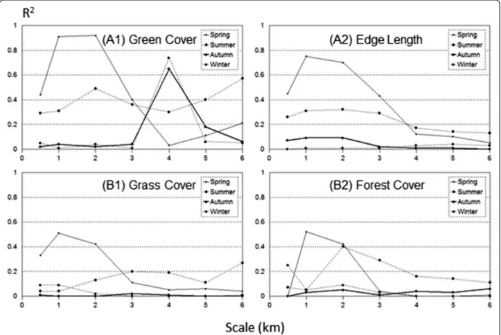
Green vegetation had the potential to reduce PM2.5 concentration in specific seasons and at some scales (Table 2). Through a simple correlation regression ana-lysis between the PM2.5 concentration and all landscape metrics (see the“Methods” section), we found that forest cover, grass cover, total green cover, and total edge length around the green covers were highly correlated with PM2.5concentration (Fig. 6). However, the strength of the correlation varied by scale and by season (Fig. 6). The PM2.5concentration appeared very highly correlated (R2> 0.85), with green cover in spring at 1–2 km scales, highly correlated (R2
> 0.6) in autumn and winter at a 4 km scale, and moderately correlated in summer (R2
> 0.4) at 2-, 5-, and 6-km scales (Fig. 6a1). For edge length, high and moderate correlations (R2
> 0.6, R2~0.35) at scales of 1–3 km were also detected between PM2.5 and total edge length during spring and summer, respectively (Fig. 6a2). Surprisingly, only a moderate correlation (R2
> 0.4) was found with both grass cover and forest cover at scales of 1.0–2.0 km (Fig. 6b1 and b2). No sig-nificant correlation was found between PM2.5 concentra-tion and total green cover when PM2.5 concentration was greater than 75μg m−3(Table 2).
Single and multiple variables were used to develop em-pirical models to predict PM2.5 concentrations for each
of the five significant scales of the corresponding seasons (Table 3). Among all the models, log(green cover) × log(edge length) as well as log(green cover) were found to be significant (Table 3). The first model was proficient in predicting spring PM2.5concentration at a 1.0–2.0 km scale, summer at a 4.0 km scale, autumn at a 6.0 km scale, and winter at a 4.0 km scale. When log(green cover) was used as the single variable, the model seemed proficient at the same season (scale). Regardless of the models’ significance, the extreme low values of the cor-relation coefficient of determination (R2
) forced us to re-ject the model when predicting PM2.5 concentration in summer, autumn, and winter. For spring, edge length alone can be used to predict PM2.5 with a confidence of 83 and 82 % at 1.0 and 2.0 km scale, respectively. Inclu-sion of green cover did not improve our predictive cap-ability (Table 4).
Discussion
Air pollution worldwide has been a consequence of in-creasing energy consumption, urban expansion, popula-tion growth, and vehicle use, which have compounded due to relatively low investments in emission control and processing technology. Extreme pollution levels have been reported in many cities, such as Los Angeles (USA), London (UK), Hong Kong (China), Milano (Italy), and now Delhi (India), Beijing (China), Mexico City (Mexico), Ulaanbaatar (Mongolia), and others in de-veloping countries (Rodrıguez et al. 2004; Apte et al. 2015; Fan et al. 2016). In Nanjing, the government
Fig. 5 Spatially interpolated mean and variation (standard error (SE)) of PM2.5concentration above/below the 75μg m−3threshold during the
issued its first-ever red alert for poor air quality on De-cember 6, 2013, due to levels of harmful PM2.5 reaching higher than 300μg m−3and lasting for more than 12 h, which reduced visibility to 1 km. This level, however, is much lower than that found in neighboring Shanghai, where a record of PM2.5 greater than 1000 μg m−3 was reported on March 28, 2014. Earlier in Shenyang, lo-cated in Northeast China, PM2.5 was detected at a
rec-ord of 1400 μg m−3—50 times above what the World
Health Organization (WHO) recommends as safe—on November 9, 2015, marking it the highest pollution on record since China began monitoring air quality in 2013. Even as this manuscript was written, Beijing issued a “Red Warning” twice in December 2015 due to the dan-gerous PM2.5 levels and required that all schools close and residents stay at home.
Smog is now an infamous term frequently used in edu-cation, policymaking, and public communities, as well as pressing issues concerning science. Of all the pollutants, PM2.5 is the most problematic because of its complex
and dangerous species composition and size. In London, a recent study found that ~9500 people die each year be-cause of air pollution (Walton et al. 2015; Zupancic et al. 2015). Apte et al. (2015) estimated that ambient PM2.5 is responsible for about 750,000 deaths annually worldwide and claimed that even a 20–30 % reduction in the average PM2.5levels over the next 15 years would merely offset the increase of PM2.5-attributed deaths in aging populations. In pursuit of sustainable urban devel-opment, societies have begun seriously seeking innovative technology, emission controls, green space enhancement (i.e., nature-based solutions), alternative policies, and other solutions (Janhäll 2015).
Green spaces in urban landscapes are increasingly recognized and promoted because of their crucial roles in urban ecosystems and human health, such as air purification, carbon sequestration, reduction of urban heat islands, and provision of recreational spaces (Chiesura 2004; Tzoulas et al. 2007; Sanesi et al. 2009; Tian et al. 2014; Wolch et al. 2014). They are
Table 2 Changes inP value from simple linear models that predict PM2.5concentration from total green cover, total edge length,
grass cover, and forest cover at seven different scales by season from July 11, 2013, through May 31, 2015 in Nanjing, China
Radius (km) Spring Summer Autumn Winter Spring Summer Autumn Winter
Green cover Edge length
0.5 0.058 0.656 0.131 0.921 0.047 0.486 0.164 0.921 1 0.005 0.772 0.092 0.882 0.003 0.441 0.120 0.870 2 0.005 0.274 0.014 0.741 0.006 0.437 0.115 0.933 3 0.039 0.830 0.049 0.890 0.053 0.702 0.133 0.807 4 0.551 0.743 0.218 0.969 0.363 0.776 0.264 0.654 5 0.830 0.567 0.847 0.790 0.405 0.829 0.322 0.602 6 0.842 0.589 0.928 0.674 0.577 0.987 0.331 0.650
Grassland cover Forest cover
0.5 0.107 0.764 0.589 0.429 0.936 0.914 0.506 0.171 1 0.041 0.972 0.628 0.433 0.028 0.653 0.583 0.560 2 0.058 0.956 0.336 0.705 0.061 0.559 0.066 0.443 3 0.378 0.703 0.232 0.898 0.590 0.776 0.133 0.659 4 0.555 0.835 0.243 0.941 0.958 0.625 0.286 0.940 5 0.511 0.934 0.206 0.902 0.906 0.640 0.326 0.996 6 0.585 0.906 0.151 0.866 0.814 0.510 0.381 0.984
Green cover (PM2.5≥ 75 ug·m−3) Green cover (PM2.5< 75 ug·m−3)
0.5 0.856 0.531 0.379 0.968 0.003 0.275 0.227 0.336 1 0.445 0.391 0.260 0.992 0.002 0.264 0.493 0.385 2 0.315 0.292 0.176 0.880 0.001 0.174 0.470 0.277 3 0.519 0.252 0.102 0.988 0.011 0.438 0.672 0.253 4 0.704 0.377 0.193 0.784 0.213 0.457 0.390 0.109 5 0.799 0.379 0.163 0.567 0.430 0.554 0.905 0.176 6 0.834 0.394 0.202 0.513 0.793 0.342 0.508 0.319
particularly effective in “capturing” pollutants through their abundant surface areas, such as leaves and bark (Nowak et al. 2013; Janhäll 2015). Our results are con-sistent with previous experiments in Nanjing (Huang et al. 2002) and elsewhere (Nowak et al. 2013; Wu et al. 2015), while our results on the negative correlation between green cover and PM2.5 concentration (Fig. 6, Table 4) support our hypothesis. However, the empir-ical relationship varies greatly by season, the degree of
PM2.5level, and the distance from the point of concern (e.g., emission source, high population concentration) (Table 2).
At first, vegetation cover of forest, grassland, and total green space seemed significant in reducing PM2.5 con-centration only within 1.0–3.0 km of a study point, not within the first 1.0 km or beyond 3.0 km. Yet, edge density within also 2.0 km appeared significant (Table 2). In other words, the PM2.5 concentration of a point in
Fig. 6 Changes in the correlation coefficient of determination (R2) between PM2.5concentration and landscape structure, with scales over four
seasons in Nanjing during 2015
Table 3P values of the two selected models for predicting PM2.5concentration from total green cover (%) and total edge length
(km) at seven scales by season in Nanjing from July 11, 2013 through May 31, 2015
Radius (km)
Spring Summer Autumn Winter Spring Summer Autumn Winter
Log(green cover)*log(edge length) Log(green cover)
0.5 0.462 0.810 0.586 0.597 0.294 0.852 0.431 0.611 1 0.009 0.651 0.684 0.845 0.050 0.679 0.911 0.842 2 0.003 0.788 0.502 0.891 0.020 0.774 0.850 0.968 3 0.385 0.800 0.412 0.903 0.562 0.744 0.582 0.880 4 0.976 0.018 0.398 0.006 0.957 0.017 0.364 0.006 5 0.432 0.367 0.091 0.667 0.457 0.327 0.097 0.721 6 0.254 0.695 0.031 0.985 0.251 0.637 0.031 0.930
the landscape can be significantly modified by dispersing smaller vegetation patches within 2.0 km as well as by the total green cover within 1.0–3.0 km. These interest-ing results need to be explored through the development of an aerodynamic footprint model (e.g., Schmid 1994), source-sink transportation, and large eddy simulations in the future. Our results can be used when managing green spaces in specific locations. Yet, if our goal is to manage the entire landscape, then increasing total cov-er—especially forest cover—and edge density are two plausible recommendations. Another outcome from these findings is that future green space promotions are possible through targeting specific emission sources (i.e., effective reduction), population sizes, and distribution (i.e., benefits to people). More so, future green space management may consider more evergreen species, es-pecially within the surrounding 2–3 km vicinity of a major emission source and other locations with high populations. Nevertheless, caution should be taken when extrapolating these results to other urban landscapes in different climate zones because of high contrasts in both landscape structure and atmospheric movement (Hao et al. 2015). Finally, the empirical models were developed with existing PM2.5 data and a static landscape. Because both dependent and independent variables can be differ-ent in the future, mechanistically based modeling is ur-gently needed.
It also appeared that the significant pollution-removal function of green spaces in Nanjing existed in spring and at some degrees in autumn (Table 2), with edges showing no obvious correlation in either summer or winter (Fig. 6). These variations among the seasons can be potentially coupled with (1) rapid changes in vegeta-tion leaves in spring and autumn and a stable amount of leaves in the summer and winter; (2) absorption of PM2.5 by rain water; and (3) high precipitation in the spring monsoon, which can wash away intercepted pol-lutants on a plant’s surface and increase wet deposition, and to some degree, dry deposition. As air moves through a landscape, pollutants are deposited on sur-faces and later fall (i.e., dry deposition) or wash away to the ground during precipitation events. This process will result in higher pollutants within forests and other green
spaces (Xu et al. 2002; Wu et al. 2008). Janhäll (2015) concluded that the “filtration vegetation barriers have to be dense enough to offer a large deposition surface area and porous enough to allow penetration.” The differences in canopy cover and the high porosity across the edges might provide partial explanations for the insignificant in-fluences in the summer and the winter. With longer edges between vegetation patches and neighboring open spaces, vegetation can potentially capture more pollutants carried through horizontal advection, resulting in higher depos-ition near the edges (Wu et al. 2015). Adddepos-itionally, the relatively humid environment (Chen et al. 1993) has a higher capacity in absorbing pollutants (i.e., wet depos-ition) (Nowak et al. 2013; Wu et al. 2015). Because PM2.5 is small in size,“capturing” them might be more effective than with other, larger particulates. Consequently, denser, taller vegetation (e.g., forests; Chen et al. 1992), higher green space coverage, and more heterogeneous vegetation patches (i.e., higher edge density) can produce stronger ef-fects on PM2.5concentration.
Lastly, the role of green spaces in PM2.5 concentration reduction varies by pollution level. A major finding of this study was the non-significant correlation between green cover and PM2.5 concentration when the concen-tration was >75μg m−3(Table 2). This suggests that the relative contribution of green spaces in PM2.5 reduction seemed low during high pollution conditions. One should not devalue the importance of green spaces when interpreting these results but instead highlight the need for field experiments to separate the contributions of vegetation among all pollution contributors (i.e., emission sources, dispersions, e.g., Chen et al. 2015). Unfortunately, such high conditions are mostly found in winter when vegetation cover is the lowest—a phenomenon found in most temperate cities (Vecchi et al. 2004; Giugliano et al. 2005; Han et al. 2015).
The underlining processes regulating PM2.5 concentra-tions in Nanjing (and within many cities) are complex and may include excessive emission from factories, rapid increase in automobiles, intensified urbanization, reduc-tion of green space, stabilizareduc-tion in air condireduc-tions, devel-opment of heat islands, and natural meteorological conditions (Huang et al. 2002; He 2010; Janhäll 2015;
Table 4 Estimated regression coefficients in five significant models predicting PM2.5concentration (Table 3) from log-transformed
independent variables of total green cover (%) and total edge length (TE, km)
Season (scale) Log(green cover)*log(edge length) Log(edge length)
Intercept Slope R2 Intercept Slope R2
Spring (1.0 km) 56.93 3.57 0.82 50.24 −10.75 0.83
Spring (2.0 km) 56.05 4.50 0.79 48.71 −12.28 0.82
Summer (4.0 km) 50.79 −0.78 0.03 49.06 −0.41 0.01
Winter (4.0 km) 100.97 −0.09 0.01 104.37 3.01 0.02
Zhang and Cao 2015). For example, the unusual higher-than-average precipitation in late February and March of 2014 may be the primary reason for its low PM2.5 con-centration (Fig. 3). During the short period of this study, the Youth Olympics Games were held in Nanjing during August 16–28, 2014. Intensified last-minute construc-tions prior to the games might have been responsible for the high PM2.5 concentration in May–July 2014, while the low concentration in August (Fig. 3) may have been a result of the government’s efforts to close many factor-ies and traffic controls several days before and during the games. Consequently, the dynamics and the level of PM2.5in the summer of 2014 were dramatically different from that in the summer of 2013. A similar policy was also implemented during December 2014 when a major memorial service was held for the Nanjing Massacre during World War II. This also resulted in lower PM2.5 levels for both the month as well as for the winter of 2014–2015, which was coupled with very unstable at-mospheric conditions (Liu et al. 2005). In this study, we
examined the dynamics of PM2.5 concentrations and
their potential effects of green vegetation but excluded many other driving mechanisms such as the above ac-tions, as well as the climatic influences—a major variable determining the transportation and deposition of all pol-lutants (Liu et al. 2005).
Our findings may not be applicable for other pollut-ants, suggesting that additional efforts are needed to ex-pand this study to other pollution species in the future. Additionally, our spatiotemporal analyses were based on a limited number of static green spaces, landscape, and available data from CNEMC—as only nine stations were aggregated in the city center (Fig. 1) during a 1.5-year study period. As more information becomes available, one needs to include detailed vegetation characteristics, which are collected through ground measurements and remote sensing, into spatially explicit models in order to understand the roles of green spaces PM2.5 concentra-tion reducconcentra-tion. Ultimately, comprehensive experiments and modeling investigations are needed so that all drivers (physical and anthropogenic) in the sources, sinks, transportation, and in the decomposition of pol-lutants are included as a scientific base for effective planning and management of green spaces in Nanjing and elsewhere.
Conclusions
In battling the increasing intensity and frequency of air pollution in urban landscapes, daily PM2.5 concentration was manually collected from the CNEMC webpage to quantify the spatiotemporal changes of PM2.5—the most dangerous pollutant affecting urban dwellings. The spa-tiotemporal changes of green spaces were further ana-lyzed at daily, weekly, monthly, and seasonal scales. We
found that PM2.5 concentrations varied by time and space. Over time, great seasonal differences existed, with winters showing the highest concentration. However, the temporal variations were interrupted by physical (e.g., the intensive monsoon in the spring of 2014) and human activities (e.g., the Youth Olympics Games in August 2014). Across the Nanjing landscape, the east and south-west have had the highest pollution levels. The non-significant correlation between green cover and PM2.5 concentration was found when its concentration was >75 μg m−3. Total edge length within 2 km of a point was significantly related to the low PM2.5 concentration. More importantly, we found that forest cover, grassland cover, total green cover, and total edge length within the 1–3 km vicinities of the monitoring station played sig-nificant roles in reducing the PM2.5 concentration, par-ticularly in spring. Although the empirical models seemed significant for spring only, one should not de-value the importance of green vegetation in other sea-sons; instead, one should understand that regulations are complicated by stable vegetation characteristics and dif-ferent meteorological conditions and human activities.
Acknowledgments
This study was primarily supported by the International Center for Ecology, Meteorology, and Environment (IceMe) of NUIST. J. Chen and P. Fan also acknowledge the funding support from the Land Cover and Land Use Program of National Aeronautics and Space Administration (NASA) through the grant to Michigan State University (NNX15AD51G). We thank Dan Wang for the discussion of the study design and results and Gabriela Shirkey for repeatedly editing the manuscript. The handling editor and three anonymous reviewers provided constructive suggestions for improving the quality of the manuscript.
Authors’ contributions
JC designed the study plan, advised the data collection and analysis, developed the entire draft manuscript, and provided the financial support for this study. LZ collected all the data, performed all data analysis, and developed all tables and figures, as well as some texts for the manuscript. PF participated in the experimental design, co-advised the scientific ques-tions, and provided many edits on the manuscript, including references and citations. LT and RL participated in research questions, landscape analysis, and edits on the manuscript’s drafts. All authors read and approved the final manuscript.
Competing interests
The authors declare that they have no competing interests. Author details
1
International Center for Ecology, Meteorology, and Environment, Nanjing University of Information Science and Technology, Nanjing 210044, China. 2CGCEO/Geography, Michigan State University, East Lansing, MI 48824, USA. 3School of Planning, Design, and Construction, Michigan State University, East Lansing, MI 48824, USA.4Institute of Geographic Sciences and Natural Resources Research, Chinese Academy of Sciences, Beijing 100101, China. 5Department of Scienze Agro-Ambientali e Territoriali, University of Bari, Bari 70126, Italy.6Department of Geography, Michigan State University, 1405 S. Harrison Road, East Lansing, MI 48823, USA.
References
Apte JS, Marshall JD, Cohen AJ, Brauer M (2015) Addressing global mortality from ambient PM2.5. Environ Sci Technol 49:8057–8066
Bartier PM, Keller CP (1996) Multivariate interpolation to incorporate thematic surface data using inverse distance weighting (IDW). Comput Geosci 22:795–799 Chen J, Franklin JF, Spies TA (1992) Vegetation responses to edge environments
in old-growth Douglas-fir forests. Ecol Appl 2:387–396
Chen J, Franklin JF, Spies TA (1993) Contrasting microclimates among clearcut, edge, and interior of old-growth Douglas-fir forest. Agr For Meteorol 63:219–237 Chen J, Saunders SC, Crow TR, Naiman RJ, Brosofske KD, Mroz GD, Brookshire BL,
Franklin JF (1999) Microclimate in forest ecosystem and landscape ecology. Bioscience 49:288–297
Chen J, Ban Y, Li S (2014) China: Open access to Earth land-cover map. Nature 514:434
Chen J, Yu X, Sun F, Lun X, Fu Y, Jia G, Zhang Z, Liu X, Mo L, Bi H (2015) The concentrations and reduction of airborne particulate matter (PM10, PM2.5, PM1) at shelterbelt site in Beijing. Atmosphere 6:650–676
Chiesura A (2004) The role of urban parks for the sustainable city. Landscape Urban Plan 68:129–138
Fan P, Chen J, John R (2016) Urbanization and environmental change during the economic transition on the Mongolian Plateau: Hohhot and Ulaanbaatar. Environ Res 144:96–112
Giugliano M, Lonati G, Butelli P, Romele L, Tardivo R, Grosso M (2005) Fine particulate (PM2.5–PM1) at urban sites with different traffic exposure. Atmos Environ 39:2421–2431
Han L, Zhou W, Li W (2015) Increasing impact of urban fine particles (PM2.5) on areas surrounding Chinese cities. Sci Rep 5:12467
Hänninen OO, Palonen J, Tuomisto JT, Yli-Tuomi T, Seppänen O, Jantunen MJ (2005) Reduction potential of urban PM2.5 mortality risk using modern ventilation systems in buildings. Indoor Air 5:246–256
Hao L, Xiao Z, Yang Q (2015) Study on planning and construction of community greenway for PM2.5 reduction. Open Fuels Energy Sci J 8:99–105 He ZJ (2010) Pollution levels of air borne particulate matter PM10and PM2.5in
summer in Nanchang city. Anhui Agri Sci 38:1336–1338
Huang LM, Wang GH, Wang H, Gao SX, Wang LS (2002) Pollution level of the airborne participate matter (PM10, PM 2.5) in Nanjing City. China Environ Sci 22:334–337
Huang YM, Shu J, Wei HP, Wang Q (2006) The estimate and GIS of fugitive dust emission from paved roads in industrial estate. Environ Sci Manage 4:673–1212 Hueglin C, Gehrig R, Baltensperger U, Gysel M, Monn C, Vonmont H (2005)
Chemical characterisation of PM2.5, PM10 and coarse particles at urban, near-city and rural sites in Switzerland. Atmos Environ 39:637–651 Hwang HJ, Yook SJ, Ahn KH (2011) Experimental investigation of submicron and
ultrafine soot particle removal by tree leaves. Atmos Environ 45:6987–6994 Janhäll S (2015) Review on urban vegetation and particle air
pollution—deposition and dispersion. Atmos Environ 105:130–137 John R, Chen J, Ou-Yang ZT, Xiao J, Becker R, Samanta A, Ganguly S, Yuan W,
Batkhishig O (2013) Vegetation response to extreme climate events on the Mongolian Plateau from 2000 to 2010. Environ Res Lett 8. doi:10.1088/1748-9326/8/3/035033
Lafortezza R, Carrus G, Sanesi G, Davies C (2009) Benefits and well-being perceived by people visiting green spaces in periods of heat stress. Urban For Urban Greening 8:97–108
Liu LZ (1985) Synoptic and climatic characteristics of the surface inversion in Nanjing region. Sci Meteorol Sinica 2:69–76
Liu X, Zhu J, Van Espen P, Adams F, Xiao R, Dong S, Li Y (2005) Single particle characterization of spring and summer aerosols in Beijing: formation of composite sulfate of calcium and potassium. Atmos Environ 39:6909–6918 Masetti M, Nghiem SV, Sorichetta A, Stevenazzi S, Fabbri P, Pola M, Filippini M,
Brakenridge GR (2015) Urbanization affects air and water in Italy’s Po Plain. Eos 96. doi:10.1029/2015EO037575
McGarigal K, Marks BJ (1994) Spatial pattern analysis program for quantifying landscape structure., USDA Gen Tech Rep PNW-GTR-351
Mugica V, Ortiz E, Molina L, De Vizcaya-Ruiz A, Nebot A, Quintana R, Aguilar J, Alcántara E (2009) PM composition and source reconciliation in Mexico City. Atmos Environ 43:5068–5074
Nowak DJ, Hirabayashi S, Bodine A, Hoehn R (2013) Modeled PM2.5 removal by trees in ten US cities and associated health effects. Environ Pollut 178:395–402 Park SS, Kim YJ (2005) Source contributions to fine particulate matter in an urban
atmosphere. Chemosphere 59:217–226
Perrone MG, Larsen BR, Ferrero L, Sangiorgi G, De Gennaro G, Udisti R, Zangrando R, Gambaro A, Bolzacchini E (2012) Sources of high PM2.5 concentrations in Milan, Northern Italy: molecular marker data and CMB modelling. Sci Total Environ 414:343–355
Querol X, Alastuey A, Ruiz CR, Artiñano B, Hansson HC, Harrison RM, Buringh ET, Ten Brink HM, Lutz M, Bruckmann P, Straehl P (2004) Speciation and origin of PM10 and PM2.5 in selected European cities. Atmos Environ 38:6547–6555 Rodrıguez S, Querol X, Alastuey A, Viana MM, Alarcon M, Mantilla E, Ruiz CR
(2004) Comparative p M10–PM2.5 source contribution study at rural, urban and industrial sites during PM episodes in Eastern Spain. Sci Total Environ 28:95–113
Rohde RA, Muller RA (2015) Air pollution in China: mapping of concentrations and sources. PLoS One 10(8), e0135749. doi:10.1371/journal.pone.0135749 Sanesi G, Padoa-Schioppa E, Lorusso L, Bottoni L, Lafortezza R (2009) Avian
ecological diversity as an indicator of urban forest functionality. Results from two case studies in Northern and southern Italy. J Arboriculture Urban For 35:53–59
Schmid HP (1994) Source areas for scalars and scalar fluxes. Bound-Lay Meteorol 67:293–318
Tian L, Chen J, Yu SX (2014) Coupled dynamics of urban landscape pattern and socioeconomic drivers in Shenzhen, China. Landscape Ecol 29:715–727 Tong MK, Gao JX, Tian MR, Ji P (2015) Subduction of PM2.5by road green space
in Beijing and its health benefit evaluation. Atmosphere 6:650–676 Tzoulas K, Korpela K, Venn S, Yli-Pelkonen V, Kaźmierczak A, Niemela J, James P
(2007) Promoting ecosystem and human health in urban areas using Green Infrastructure: a literature review. Landscape Urban Plan 81:167–178 Vecchi R, Marcazzan G, Valli G, Ceriani M, Antoniazzi C (2004) The role of atmospheric dispersion in the seasonal variation of PM1 and PM2.5 concentration and composition in the urban area of Milan (Italy). Atmos Environ 38:4437–4446
Vecchi R, Marcazzan G, Valli G (2007) A study on nighttime–daytime PM10 concentration and elemental composition in relation to atmospheric dispersion in the urban area of Milan (Italy). Atmos Environ 41:2136–2144 Viana M, Kuhlbusch TA, Querol X, Alastuey A, Harrison RM, Hopke PK, Winiwarter
W, Vallius M, Szidat S, Prévôt AS, Hueglin C (2008) Source apportionment of particulate matter in Europe: a review of methods and results. J Aersol Sci 39: 827–849
Walton H, Dajnak D, Beevers S, Williams M (2015) Understanding the health impacts of air pollution in London. King’s College London, UK, p 129 Wolch JR, Byrne J, Newell JP (2014) Urban green space, public health, and
environmental justice: the challenge of making cities‘just green enough’. Landscape Urban Plan 125:234–244
Wu ZP, Wang C, Hou XJ, Yang WW (2008) Variation of air PM2.5 concentration in six urban greenlands. J Anhui Agri Univ 35:494–498
Wu J, Xie W, Li W, Li J (2015) Effects of urban landscape pattern on PM2.5 pollution—a Beijing case study. PLoS One 10(11), e0142449
Xu H, Deng B, Zhou X, Wang Q (2002) Effect of fog on urban boundary layer and environment. J Appl Meteorol Sci 13:170–176
Zhang YL, Cao F (2015) Fine particulate matter (PM2.5) in China at a city level. Sci Rep 5:14884
Zupancic A, Westmacott C, Bulthuis M (2015) The impact of green space on heat and air pollution in urban communities: a meta-narrative systematic review. David Suzuki Foundation, Vancouver, BC, Canada, p 67
Submit your manuscript to a
journal and benefi t from:
7 Convenient online submission 7 Rigorous peer review
7 Immediate publication on acceptance 7 Open access: articles freely available online 7 High visibility within the fi eld
7 Retaining the copyright to your article