DiSES Working Papers
Università degli Studi di Salerno Dipartimento di Scienze Economiche e Statistiche >>>www.dises.unisa.it
Bias-corrected inference
for multivariate nonparametric regression:
model selection and oracle property
Francesco Giordano
Maria Lucia Parrella
ISSN: 1971-3029
Dipartimento di Scienze Economiche e Statistiche Università Degli Studi di Salerno
Via Ponte Don Melillo – 84084; Fisciano (SA) – Italy
Tel +39-089-96.21.55 Fax +39-089-96.20.49 E-mail [email protected]
BIAS-CORRECTED INFERENCE FOR MULTIVARIATE NONPARAMETRIC REGRESSION: MODEL SELECTION AND
ORACLE PROPERTY
Francesco Giordano∗ Maria Lucia Parrella†
Abstract. The local polynomial estimator is particularly affected by the curse of
di-mensionality. So, the potentialities of such a tool become ineffective for large dimensional
applications. Motivated by this, we propose a new estimation procedure based on the lo-cal linear estimator and a nonlinearity sparseness condition, which focuses on the num-ber of covariates for which the gradient is not constant. Our procedure, called BID for
Bias-Inflation-Deflation, is automatic and easily applicable to models with many
covari-ates without any additive assumption to the model. It simultaneously gives a consistent estimation of a) the optimal bandwidth matrix, b) the multivariate regression function and
c) the multivariate, bias-corrected, confidence bands. Moreover, it automatically identify the relevant covariates and it separates the nonlinear from the linear effects. We do not need pilot bandwidths. Some theoretical properties of the method are discussed in the paper. In particular, we show the nonparametric oracle property. For linear models, the BID automatically reaches the optimal rateOp(n−1/2), equivalent to the parametric case.
A simulation study shows a good performance of the BID procedure, compared with its direct competitor.
Keywords: multivariate nonparametric regression, multivariate bandwidth selection, mul-tivariate confidence bands.
AMS 2010 classifications: 62G08, 62G05, 62G15, 62G10, 62H99. JEL classifications: C14, C15, C18, C88.
Acknowledgements: The authors thank professor S.N. Lahiri for helpful comments on this work. This work has been partially supported by the PRIN research grant “La pre-visione economica e finanziaria: il ruolo dell’informazione e la capacità di modellare il cambiamento” - prot. 2010J3LZEN005.
The authors gratefully acknowledge support from the University of Salerno grant pro-gram “Sistema di calcolo ad alte prestazioni per l’analisi economica, finanziaria e statistica (High Performance Computing - HPC)” - prot. ASSA098434, 2009".
1. Introduction
Let(X1, Y1), . . . , (Xn, Yn) be a set of Rd+1-valued random vectors, where theYi are the
dependent variables and theXiare the Rd-valued covariates of the following model
Yi = m(Xi) + εi. (1)
∗DISES, Via Ponte Don Melillo, 84084, Fisciano (SA), Italy, [email protected] †DISES, Via Ponte Don Melillo, 84084, Fisciano (SA), Italy, [email protected]
The functionm(Xi) = E(Yi|Xi) : Rd→ R is the multivariate conditional mean function.
The errorsεi are assumed to be i.i.d. and independent ofXi. We use the notationXi =
(Xi(1), . . . , Xi(d)) to refer to the covariates and x = (x1, . . . , xd) to denote the target
point at which we want to estimatem. We indicate with fX(x) the density function of
the covariate vector, having supportsupp(fX) ⊆ Rdand assumed to be positive. Besides,
fε(·) is the density function of the errors, assumed to be N(0, σε2).
Our goal is to estimate the functionm(x) = E(Y |X = x) at a point x ∈ supp(fX),
supposing that the parametric form of the functionm is completely unknown without im-posing any additive assumption. We assume that the number of covariatesd is high but only some covariates are relevant. The analysis of this framework raises the problem of the curse
of dimensionality, which usually concerns nonparametric estimators, and consequently the
problem of variable selection, which is necessary to pursue dimension reduction.
In the last years, many papers have studied this nonparametric framework. A good re-view is given in Comminges and Dalalyan (2012). For variable selection, we mention the penalty based methods for semiparametric models of Li and Liang (2008) and Dai and Ma (2012); the neural network based method of La Rocca and Perna (2005); the empirical based method of Variyath et al. (2010). Some other methods contextually perform variable selection and estimate the multivariate regression function consistently. See, for example, the COSSO of Lin and Zhang (2006), the ACOSSO of Storlie et al. (2011), the LAND of Zhang et al. (2011) and the RODEO of Lafferty and Wasserman (2008). All these methods are appealing for their approaches, but some typical drawbacks are: the difficulty to ana-lyze theoretically the properties of the estimators; the computational burden; the difficulty to implement the procedures, which generally depend crucially on some regularization pa-rameters, quite difficult to set; the necessity of considering stringent assumptions on the functional space (for example, imposing an additive model).
The aim of this paper is to propose a nonparametric multivariate regression method which mediates among the following priorities: the need of being automatic, the need of scaling to high dimension and the need of adapting to large classes of functions. In order to pur-sue this, we work around the local linear estimator and its properties. Our work has been inspired by the RODEO method of Lafferty and Wasserman (2008). As a consequence, some of the theoretical results presented in Lafferty and Wasserman (2008) have repre-sented the building blocks of our research. In particular, we borrow the idea of using an iterative procedure in order to “adjust” the multivariate estimation one dimension at a time. Anyway, the BID procedure substantially works differently from the RODEO, since they have different targets. In the RODEO procedure, a technique is proposed in order to check the relevance of the covariate, which is iteratively repeated along each relevant dimension and along a grid of decreasing bandwidths, in order to find the correct order of the band-width matrix. In this way, it performs (nonlinear) variable selection, bandband-width selection and multivariate function estimation. However, it also leaves some unresolved issues. First of all, it does not identify the relevant linear covariates. Moreover, it does not estimate the optimal bandwidth matrix, so its final function estimation is not the optimal one. Finally, it can be applied only with uniform covariates whereas our method can be extended to non-uniform designs. In addition, we improve the rate of convergence of the final estimator, as in Comminges and Dalalyan (2012) and Bertin and Lecué (2008)).
In particular, the contributions of this paper are described in the following.
which is completely automatic and easily applicable to models with many covariates. It is based on the assumption that each covariate may have a different bandwidth value. Note that the bandwidths have a central role in the proposed BID procedure, since they are used to make variable selection and model selection as well;
• our method has the nonparametric oracle property, as defined in Storlie et al. (2011). In particular, it selects the correct subset of predictors with probability tending to one, and estimates the non-zero parameters as efficiently as if the set of relevant covariates were known in advance. Moreover, it automatically separates the linearities from the nonlinearities. We show that the rate of convergence of the final estimator is not sensitive to the number of relevant linear covariates involved in the model (i.e., those for which the partial derivative is constant with respect to the same covariate), even when the model is not additive. As a consequence, the effective dimension of the model can increase, without incurring in the curse of dimensionality, as long as the number of nonlinear covariates (i.e., those whose partial derivative is not constant with respect to the same covariate) is fixed;
• our procedure includes a consistent bias-corrected estimator for the multivariate re-gression function, and also for its multivariate confidence bands. These can be used, for example, to make model selection.
• the proposed method does not need any regularization parameter, contrary to LASSO based techniques, and it does not use any additive assumption.
In the next section we introduce the notation. The BID algorithm is presented in sec-tion 3. In secsec-tion 4, we propose a method for the estimasec-tion of the optimal bandwidth matrix, while section 5 presents the estimators of the functionals for the derivation of the bias-corrected multivariate confidence bands. Section 6 contains the theoretical results. In section 7 we show a way to remove the uniformity assumption for the design matrix. A simulation study concludes the paper. The assumptions and the proofs are collected in the appendix.
2. Fundamentals of the Local Linear estimators
The BID smoothing procedure is based on the use of the local linear estimator (LLE). The last is a nonparametric tool whose properties have been deeply studied. See Ruppert and Wand (1994), among others. It corresponds to perform a locally weighted least squares fit of a linear function, equal to
arg min β n ∑ i=1 { Yi− β0(x) − βT1(x)(Xi− x)} 2 KH(Xi− x) (2)
where the functionKH(u) = |H|−1K(H−1u) gives the local weights and K(u) is the
Kernel function, ad-variate probability density function. The d × d matrix H represents the smoothing parameter, called the bandwidth matrix. It controls the variance of the Kernel function and regulates the amount of local averaging on each dimension, and so the local smoothness of the estimated regression function. Denote with β(x) = (β0(x), βT1(x))T
the vector of coefficients to estimate at pointx. Using the matrix notation, the solution of the minimization problem in (2) can be written in closed form
ˆ
where ˆβ(x; H) = ( ˆβ0(x; H), ˆβ T
1(x; H))T is the estimator of the vector β(x) and
Υ = Y1 .. . Yn , Γ = 1 (X1− x)T .. . ... 1 (Xn− x)T , W = KH(X1− x) . . . 0 .. . . .. ... 0 . . . KH(Xn− x) . Let Dm(x) denote the gradient of m(x). Note from (2) that ˆβ(x; H) gives an estimation
of the functionm(x) and its gradient. In particular, ˆ β(x; H) =( ˆβˆ0(x; H) β1(x; H) ) ≡ ( ˆ m(x; H) ˆ Dm(x; H) ) . (4)
Despite its conceptual and computational simplicity, the practical implementation of the LLE is not trivial in the multivariate case.
One of the difficulties of the LLE is given by the selection of the smoothing matrix H, which crucially affects the properties of the local polynomial estimator. An optimal bandwidthHopt exists and can be obtained taking account of the bias-variance trade-off. In order to simplify the analysis, often H is taken to be of simple form, such as H = hId or H = diag(h1, . . . , hd), where Id is the identity matrix, but even in such cases
the estimation of the optimal H is difficult, because it is computationally cumbersome and because it involves the estimation of some unknown functionals of the process. As a consequence, few papers deal with this topic in the multivariate context (among which Ruppert (1997) and Yang and Tschernig (1999)). One of the contributions of this paper is to propose a novel method for the estimation of the multivariate optimal bandwidth which can be efficiently implemented with many covariates. It is described in sections 4 and 5.
A second problem with the LLE is its bias. In particular, supposing thatx is an interior point andH = diag(h1, . . . , hd), we know from Theorem 2.1 in Ruppert and Wand (1994)
that the main terms in the asymptotic expansion of the bias and variance are
Abias{ ˆm(x; H)|X1, . . . , Xn} = 1 2µ2 d ∑ j=1 ∂2m(x) ∂xj∂xj h2j (5) Avar{ ˆm(x; H)|X1, . . . , Xn} = ρ0σ2ε nfX(x)∏dj=1hj , (6)
whereµ2andρ0are moments of the Kernel function, defined as
µr =
∫
ur1K(u)du, ρr=
∫
ur1K2(u)du, r = 0, 1, 2, . . . .
Note from (5) that the bias is influenced by the partial derivatives ofm with respect to all the regressors. So, for a finiten, there is a bias component which makes the tests and the confidence intervals based on the LLE not centered around the true value of the function m(x), even when the bandwidth matrix is the optimal one. As a consequence, some bias correction should be considered in order to calibrate the nonparametric inference based on the LLE, but this is difficult to obtain. There are few papers which consider some kind of bias reduction of the multivariate LLE, among which Lin and Lin (2008) and Choi et al. (2000). An interesting contribution of the BID procedure is that it produces a bias corrected estimation of the multivariate functionm(x) and its multivariate confidence bands. We explain how in section 5.
1. Define the bias-inflating bandwidthHU = diag(hU, . . . , hU), where hU is a relatively
high value (for example, 0.9).
2. Initialise the sets of covariatesC = {1, 2, . . . , d} and A = ∅.
3. For each covariateX(j), j ∈ C, do:
a) usingHU, compute the statisticZjand the thresholdλj, by (7) and (8)
b) if|Zj| > λjthen (nonlinear covariate):
– define the bias-deflating bandwidth matrix HL =
diag(hU, . . . , hL, . . . , hU), which is equal to HU except for position
(j, j), where hLis a relatively small value (for examplehL= hUd/n)
– using HU andHL, estimate the marginal bias ˆbj(x, K) and the optimal
bandwidth ˜hj, as shown in sections 4 and 5
else
– set ˜hj= hU, ˆbj(x, K) = 0 and move the covariate j from C to A
4. For each covariateX(j), j ∈ A, do:
a) using ˜H = diag(˜h1, . . . , ˜hd), compute the statistic Nj and the thresholdωj, by
equations (9) and (10)
b) if|Nj| < ωjthen (irrelevant covariate) remove the covariatej from A
5. Output:
a) the final estimated optimal bandwidth ˜H = diag(˜h1, . . . , ˜hd)
b) the bias corrected estimatem(x; ˜ˆ H) −∑dj=1ˆbj(x, K)˜h2j
c) the sets of nonlinear covariatesC and linear covariates A.
Table 1: The basic BID smoothing algorithm
3. The BID method
The main idea of our procedure is to “explore” the multivariate regression function, search-ing for relevant covariates. These are divided into: a) the set of nonlinear covariates and b) the set of linear covariates. The covariates are defined linear/nonlinear, depending on the marginal relation between the dependent variable and such covariates, measured by a partial derivative which is constant/nonconstant with respect to the covariate itself.
The box in table 1 reports the steps of the basic algorithm used to analyse the case when all the covariates follow a Uniform distribution, assuming the hypotheses (A1)-(A6) re-ported in the appendix. In section 7 we extend the applicability of the procedure to those setups where the covariates are not uniformly distributed.
The name BID is an acronym for Bias-Inflation-Deflation. The reason for this name to the procedure is the following. The basic engine of the procedure is a double estimation for each dimension, which is included in step 3b and described in detail in sections 4 and 5. In the first estimation, of bias-inflation, we fix all the bandwidths equal to a large valuehU,
such that we oversmooth along all the directions (note that this is equivalent to estimating locally an hyperplane). In the second estimation, of bias-deflation, we consider a second estimation with a small bandwidthhL<< hU, such that we undersmooth. The comparison
between the two estimations allows to determine the right degree of “peaks” and “valleys” for the nonlinear directions, whereas the linear directions remain oversmoothed.
Before describing the procedure in detail, some preliminary considerations are necessary. First of all, it is known that the LLE are usually analyzed under the assumption that∥H∥ → 0 when n → ∞ (so the bandwidths of all the covariates must tend to zero for n → ∞). This is required in order to control the bias ofm(x; H), so that it can be asymptotically zero.ˆ Anyway, we show in Lemma 2 that the bias ofm(x; H) does not depend on the bandwidthsˆ of the linear covariates, because for such covariates the second partial derivative is zero (so the sum in (5) is actually to be taken forj ∈ C). So, in order to gain efficiency, the BID lets the bandwidths of the linear covariates to remain large, while only the bandwidths of the nonlinear covariates tend to zero forn → ∞ (see Theorem 1).
The BID procedure performs variable selection through steps 3b and 4b. In particular, step 3b concerns the identification of the nonlinear covariates, by means of the derivative expectation statisticZj proposed in Lafferty and Wasserman (2008). It is equal to
Zj = ∂ ˆm(x; H) ∂hj = eT1BLj(I − Γ B) Υ, (7) where Lj = diag (∂ log K((X 1j−xj)/hj) ∂hj , . . . , ∂ log K((Xnj−xj)/hj) ∂hj )
, e1 is the unit vector
with a one in the first position andB = (ΓTW Γ)−1ΓT W. The statistic in (7) reflects the sensitivity of the estimatorm(x; H) to the bandwidth of X(j), so it is expected to takeˆ non-zero values for the nonlinear covariates and null value otherwise. Using the results shown in Lafferty and Wasserman (2008), the threshold can be fixed to
λj =
√ ˆ σ2
εeT1GjGTje12 log n, j = 1, . . . , d, (8)
whereGj = BLj(I − Γ B) and ˆσε2 is some consistent estimator ofσ2ε. After step 3b, the
setA = C contains both the linear and irrelevant covariates. In order to separate them, step 4b performs a threshold condition on the partial derivative coefficients, basing on
Nj ≡ bD(j)m (x; ˜H) = ej+1B Υ,˜ j ∈ C, (9)
where ˜B is the same matrix as B replacing the bandwidth matrix H with the estimated one, ˜
H.
Such a statistic is expected to be approximately equal to zero for irrelevant covariates. The normal asymptotic distribution of the local polynomial estimator, shown in Lu (1996), can be used to derive the threshold
ωj =
√ ˆ σ2
εeTj+1B ˜˜BTej+12 log n, (10)
The statistics in (9) and its distribution derive from well-established results. In particular, the threshold (10) is based on the tail bounds for Normal distribution. One can show that P (|Nj| > ωj) → 0 when n → ∞ if the covariate j is irrelevant. But note that such
tests are performed using the estimated bandwidth ˜H, which does not satisfy the classic assumption∥H∥ → 0. A theoretical justification of our proposal is thus required and it is given in Lemma 2 (see the appendix). In particular, we show that the bandwidthshj,
when j is an irrelevant covariate, do not influence the bias of the estimator bD(j)m (x; ˜H), under the assumptions (A1)-(A6). Therefore, such bandwidths can be fixed large, to gain efficiency. This is what is done through the estimated matrix ˜H (see sections 4 and 5). In the same way, forj a linear covariate, the bias of the estimator bD(j)m(x; ˜H), under the assumptions (A1)-(A6), does not depend onhj. So we can also fix large the bandwidths
4. The optimal bandwidth matrix
In this section we propose a methodology to estimate the multivariate optimal bandwidth, when it is assumed to be of typeH = diag(h1, . . . , hd). Here we assume, for simplicity,
that the nonlinear covariates are the firstk regressors X(1), . . . , X(k).
When considering a givenn, the optimal multivariate bandwidth Hopt must be chosen taking account of the bias-variance trade-off. It is defined as
Hopt= arg min
H
[
Abias2{ ˆm(x; H)} + Avar{ ˆm(x; H)}],
where, for simplicity, we omit the conditioning onX1, . . . , Xn from the notation. It is
known that a simple solution is available if we assume thatH = hId. It is given by
hopt = dρ0σε2 nfX(x) [ µ2∑dj=1 ∂m(x) ∂xj∂xj ]2 1/(d+4) . (11)
Clearly, the assumption of a common bandwidth for all the dimensions is unsatisfactory, because some of the covariates are assumed to be irrelevant but also because we can observe different curvatures of the functionm(x) along the d directions. On the other side, the assumption of a diagonal matrixH with different bandwidths for the covariates is more realistic, but difficult to deal with when considering its estimation.
The bandwidth selection method proposed here is based on the idea of “marginalizing” theAM SE. Let us reformulate (5) and (6) as functions of the bandwidth hj, conditioned to
the other bandwidthsi ̸= j = 1, . . . , d. Denote with H(j) = (h1, . . . , hj−1, hj+1, . . . , hd)
the vector of the “given” bandwidths, forj = 1, . . . , d. For the asymptotic bias we have
Abias{hj|H(j)} = 1 2µ2 d ∑ i̸=j ∂2m(x) ∂xi∂xi h2i +1 2µ2 ∂2m(x) ∂xj∂xj h2j (12) = a(x, K, H(j)) + bj(x, K)h2j (13)
wherea(x, K, H(j)) =∑di̸=jbi(x, K)h2i represents the bias cumulated on the axesi ̸= j.
For the variance we have
Avar{hj|H(j)} = ρ0σε2 f (x)∏di̸=jhi 1 nhj = c(x, K, H(j)) 1 nhj , (14)
from which the definition ofc(x, K, H(j)) can be clearly deduced. The behaviour of the functions in (13) and (14) are shown in figure 1, plots (a) and (b). The marginal asymptotic mean square error becomes
AM SE{hj|H(j)} = [ a(x, K, H(j)) + bj(x, K)h2j ]2 + c(x, K, H(j)) 1 nhj (15) and the optimal value of the bandwidthhj is
hoptj = arg min
hj AM SE{h
j|H(j)}, j = 1, . . . , d.
hL
A
v
ar(hL)
VL
(a) Asymptotic variance
hL hU Abias(hL) Abias(hU) AL BUL (b) Asymptotic bias hL hU m(x) BUL (c) BID mechanism
Figure 1: Asymptotic variance (a) and bias (b) of the local linear estimatormˆ(x; H), as a function of the marginal bandwidth hj. Plot (c) shows the BID mechanism, which derives from the comparison between the
LP estimations obtained with the two bandwidths hLj << hUj.
the covariateX(j) is a linear covariate, that is when ∂m(x)/∂xj = C1, for some value
C1 ̸= 0 not dependent on X(j). In such case bj(x, K) ≡ 0 and the (15) is minimized for
hj infinitely large. The second case is when the covariateX(j) is irrelevant. Note that an
irrelevant covariate is a special linear covariate, for which∂m(x)/∂xj = C1 ≡ 0, so the
optimal bandwidth is again infinitely large. The last case is when the variableX(j) is a
nonlinear covariate, that is forj = 1, . . . , k. In such a case (and only in such a case), the
optimal bandwidth must be estimated by solving the following equation ∂ Abias2{h j|H(j)} ∂hj = − ∂ Avar{hj|H(j)} ∂hj . (16)
In order to solve the (16), we need to approximate in some way the asymptotic bias and variance of the LLE. For example, the cross-validation methods approximate the mean square error by estimating it on a grid of bandwidths and then find the optimal value by minimizing such estimated curve with respect toH. This method is impracticable in mul-tivariate regression, both theoretically and computationally. On the other side, we propose a method which is easily applicable to high dimensional models.
First of all, consider the variance functional in (14). As a function ofhj, its behaviour is
depicted in plot (a) of figure 1. Given the (14), we can approximate a generic point of the curve by knowing the value of the function for a given bandwidthhj. In particular, if we
fix a low value of the bandwidthhL, the asymptotic variance will be Avar{hL|H(j)} = c(x, K, H(j))
1
nhL. (17)
From the (17) we can derive a value forc(x, K, H(j)) and reformulate the (14) as
Avar{hj|H(j)} = Avar{hL|H(j)} hL hj = VL j hL hj . (18)
Now consider the bias functional in (13). As a function ofhj, its behaviour is depicted in
plot (b) of figure 1. We follow the same arguments as before in order to approximate the asymptotic bias function. Suppose to fix an upper value of the bandwidthhU >> hLand to evaluate the function for the two values of bandwidthshLandhU. We have
We can reformulate the (13) as follows
Abias{hj|H(j)} = a(x, K, H(j)) +Abias{h
U|H (j)} − Abias{hL|H(j)} (hU)2− (hL)2 h 2 j = AL j + BjU L (hU)2− (hL)2h 2 j. (20)
From the (16), (18) and (20) we obtain
4 [ BU L j (hU)2− (hL)2 ]2 h5j + 4A L j BjU L (hU)2− (hL)2h 3 j − VjLhLj = 0 (21)
which represents the estimation equation for the optimal bandwidthhoptj . The following Lemma is shown in the appendix.
Lemma 1 (Optimal bandwidth matrix). There is a unique real positive solution to the
following system of equations
4 [ BU L 1 (hU)2−(hL)2 ]2 h5 1+ 4AL 1 B1U L (hU)2−(hL)2h31− V1LhL= 0 .. . 4 [ BU L k (hU)2−(hL)2 ]2 h5 k+ 4AL k BU Lk (hU)2−(hL)2h3k− VkLhL= 0
with respect to the variablesh1, . . . , hk, wherek < d is the number of nonlinear covariates
in model (1). Such a solution identifies the multivariate optimal bandwidth matrixHopt =
diag(hopt1 , . . . , hoptk ).
5. Estimation of the bias-variance functionals
Following the idea of the plug-in method, we can estimate the marginal optimal bandwidth plugging into the (21) an estimation of the unknown functionals, and then solving the equa-tion with respect tohj. We can note that the unknown quantities, which are graphically
evidenced in figure 1, are BU L j = Abias{hU|H(j)} − Abias{hL|H(j)} (22) ALj = Abias{hL|H(j)} = ∑ i̸=j bi(x, K)h2i (23) VjL = Avar{hL|H(j)} (24)
and these functionals can also be used to derive the bias-corrected multivariate confidence bands for the function m(x), using the asymptotic normality of the LLE shown in Lu (1996). So, using our BID smoothing procedure, the estimation of the multivariate band-widthH and the estimation of the multivariate bias-corrected confidence bands of m(x) have a common solution: the estimation of the functionals in (22)-(24).
Figure 1 explains the idea underlying our proposal for the estimation of these functionals. Plots (a) and (b) show a typical behavior of the asymptotic mean square error of the local linear estimator, for a given axis1 ≤ j ≤ k. For a large value of the bandwidth (hj = hU),
the variance is low but there is much bias (so this is a situation of bias-inflation). On the other side, when the bandwidth is low (hj = hL), a large variance of the estimator is
compensated by its low bias (so this is a situation of bias-deflation). This is more clearly evidenced by the two box-plots shown in plot (c) of Figure 1, which summarize the typ-ical distributions of the local linear estimations ofm(x) for a relevant number of Monte Carlo replications, considering respectively the two bandwidthshLandhU. Note that the
difference between the medians of the two boxplots reflects the increment in the expected value of the bias observed when increasing the bandwidthhj fromhLtohU. Therefore it
is proportional toBU L
j . So, the comparison between the two estimations determines what
we call the Bias-Inflation-Deflation mechanism.
Following this idea, for the estimation ofBjU Lwe consider the two bandwidth matrices HU = diag(hU, . . . , hU, . . . , hU)
HLj = diag(hU, . . . , hL, . . . , hU)
which differ only for the value in position(j, j), with j ∈ C, respectively equal to hU and hL. Given (19) and Lemma 2 (see the appendix), we can show that
E[m(x; Hˆ U) − ˆm(x; HLj)|X1, . . . , Xn]
= Abias{ ˆm(x; HU)} − Abias{ ˆm(x; HLj)} + Op(n−1/2)
≈ bj(x, K)[(hU)2− (hL)2]= BjU L
therefore we propose the following estimator of the biasbj(x, K) for the axis j
d BU L j = m(x; Hˆ U) − ˆm(x; HLj), j = 1, . . . , k (25) ˆbj(x, K) = d BU L j [(hU)2− (hL)2]. (26)
Following the suggestion in Fan and Gijbels (1995), we use the following estimator of the functionalVjL c VL j = ˆσε2eT1(ΓT WjLΓ)−1ΓT WjLWLj Γ(ΓT WLj Γ)−1e1, j = 1, . . . , k (27) whereWLj = diag(KHL j(X1− x), . . . , KHLj(Xn− x) )
andσˆ2ε is some consistent esti-mator ofσε2(see, for example, the estimator proposed in Lafferty and Wasserman (2008)).
Finally, we note from the (23) that the functionalAL
j depends on the values of the
band-widthshi and the biasesbi(x; K) generated on the axes i ̸= j. For this reason, we must
consider a preliminary step for the estimation of such values. These are obtained consider-ingk univariate bandwidth estimation problems, setting AL
j = 0 in the (21) 0hˆoptj = c VL j hL 4 (hU)2− (hL)2 d BU L j 2 1/5 j = 1, . . . , k.
Now we solve the system of equations in Lemma 1 after plugging the previous estimation ofBU L
j andVjLproposed in (25) and (27), and the following estimation ofALj
sAcLj = k ∑ i̸=j s−1ˆh2i d BU L i (hU)2− (hL)2, s = 1, 2, . . . (28)
and then we iterate (increasings) until convergence. This represents a numerical step which does not require any further kernel estimations, so it is very fast. Our practical experience from the simulation study shows that the convergence is reached in few steps. Note that the componentALj implies a correction of the optimal bandwidth, by means of the second term in the (21), to take account of the interconnections among the variables. When this component is equal to zero, the formula of the optimal bandwidthhoptj is equivalent to the one derived in the univariate regression.
Remark 1: the bandwidth estimation procedure proposed here follows a marginalized ap-proach. Anyway, note that the estimated bandwidths are consistent with the optimal mul-tivariate bandwidthHopt derived with no marginalization. In other words, the estimation procedure, described in this section, is consistent in the sense that it gives the same solu-tions as in Lemma 1 (see Theorem 1). Moreover, this procedure suggests a fast algorithm to solve the non-linear system in Lemma 1.
6. Theoretical results
In this section we present the theoretical results which justify the BID procedure. In par-ticular, Theorems 1 and 2 together with Remark 2, show the consistency and the rate of convergence in the case of uniform covariates, while Theorems 3 and 4 (see section 7) will consider the non-uniform case.
Considering model (1), let ˜H be the matrix with the final estimated bandwidths and ˜Hk
be the submatrix with the final estimated bandwidths for the nonlinear covariates, assumed to be (for simplicity) the first k on the diagonal of ˜H, that is ˜Hk = diag(˜h1, . . . , ˜hk).
Moreover, assume thatHoptk is the diagonal matrix with the optimal bandwidths for suchk
nonlinear covariates. The following two Theorems hold.
Theorem 1 (consistency in selection). Assume that the assumptions (A1)-(A6), reported in
the appendix, hold withs = 4. Then we have
P(˜hj = hU, for allj > k ) → 1 n → ∞ (˜h1, . . . , ˜hk) = Op ( n−1/(4+k)). Furthermore, ˜Hk(Hoptk )−1 p
−→ Ik, where the convergence in probability is componentwise
withIkthe identity matrix of orderk.
Remark 2: (Oracle property: consistency in selection) By Theorem 1 we have thatP ( ˆC = C) → 1 as n → ∞, with ˆC and C the sets of estimated nonlinear covariates and true ones, respectively. Using the same assumptions as in Theorem 1 withs = 5, it follows that
P ( ˆA = A) → 1, n → ∞,
where ˆA and A are the sets of estimated linear covariates and true ones, respectively (see Table 1, step 4b). This result follows straightforward by applying Lemma 2 and Corollary 1 and the same arguments as in the proofs of Lemmas 7.1, 7.4 and 7.5 in Lafferty and Wasserman (2008). Therefore, Theorem 1 and this Remark lead to the first part of the Oracle property (consistency in selection).
Theorem 2 (Oracle property: rate of convergence). Under the assumptions of Theorem (1), we have [ ˆ m(x; ˜H) − m(x)]2 = Op ( n−4/(4+k)).
Note from Theorem 2 that only the nonlinear covariates inC have a strong influence on the rate of convergence, since they represent the only dimensions for which the bandwidths shrink the support of the local regression, reducing the number of usable observations. The other bandwidths remain large, so the efficiency of the estimation procedure remarkably improves. As a consequence, in order to avoid the curse of dimensionality, we must assume that the number of nonlinear covariatesk is fixed and relatively small, while the number of relevant variablesr can diverge. Note that if m(x) is a linear model (k = 0), then the BID estimator reaches the rateOp(n−1) which is equivalent to the parametric case. Moreover,
this result is valid for general models, including the mixed effect terms.
Remark 3: (diverging number of covariates) The proposed selection method as in Theorem 1 and Remark 2 can be extended to the case when the number of covariates, d → ∞. Suppose thatk = O(1), r ≤ d and d = O(log log nlog n ), the results of Theorem 1 and Remark 2 are still valid using the same arguments as in the proof of Lemma 7.1 in Lafferty and Wasserman (2008). It implies that the number of linear covariates can diverge at the same order asd.
7. Extension to non-uniform designs
The test used in step 3a is based on the fundamental assumption that the covariates are uni-formly distributed. The reason why this assumption is so crucial can be understood from Lemma 7.1 and Remark 7.2 in Lafferty and Wasserman (2008). In few words, the uni-formity assumption simplifies the asymptotic analysis of the local linear estimator, which is particularly hard if one takes into account the unusual assumption that, for some di-mensions, the bandwidth may not tend to zero whenn → ∞. In order to overcome this problem, and to extend the applicability of both the BID and the RODEO procedures, we propose to consider a transformation of model (1).
LetFjdenote the univariate marginal distribution function ofX(j), let Fj−1be its inverse
andfj its density function. Consider the transformed vector of covariatesUi = FX(Xi),
where the functionFX(Xi) : Rd→ Rdis defined as follows
FX(Xi) = (F1(Xi(1)), . . . , Fd(Xi(d))).
Model (1) can be rewritten as
Yi= m(F−1X (Ui)) + εi = g(Ui) + εi, (29)
whereg = m · F−1X andUi is uniformly distributed on the unit cube. Consider the
trans-formed point of estimationu = FX(x) and note that
∂g(u) ∂uj = ∂m(x) ∂xj 1 fj(uj) , j = 1, . . . , d. (30)
Now, supposing that fj(uj) > 0, the partial derivatives in (30) are equal to zero if and
x. So, g(u) ≡ m(x) and the function g depends on the same covariate as the function m. Therefore, both the problems of multivariate function estimation and variable selection can be solved equivalently using models (1) and (29), but the fundamental difference is that model (29) satisfies the assumptions (A1)-(A6) reported in the appendix. So, the basic BID procedure can be applied consistently replacing the covariates X(j) with U (j) = Fj(X(j)), for j = 1, . . . , d, and considering model (29). We call the last case the general
BID procedure. There are some drawbacks to be taken into account. The first one is that the transformed model (29) does not have the same structure as the original model, since, for example, the linear covariates of model (1) generally become nonlinear covariates in model (29). So the two models cannot be used equivalently for model selection. The other drawback is that the distribution functionsFj, needed to transform model (1), are unknown.
We can estimate them through the corresponding empirical distribution functions ˆFj, but
this introduces additional variability in the final estimations, due to the estimation error of Fj. Now, we present the theoretical results that justify the generalised version of the BID
procedure.
Considering model (29), let ˜H be the matrix with the final estimated bandwidths and ˜
Hrbe the diagonal matrix with the final estimated bandwidths for the relevant covariates,
assumed to be the first r on the diagonal of ˜H, that is ˜Hr = diag(˜h1, . . . , ˜hr). Finally,
assume thatHoptr is the diagonal matrix with the optimal bandwidths for suchr relevant
covariates. The following two Theorems hold.
Theorem 3 (consistency). Assume that the assumptions (A1)-(A5), reported in the
ap-pendix, hold withs = 5. Moreover, assume that the Kernel function has a bounded first
derivative and the density functions,fj(·), j = 1, . . . , d, have a bounded fourth derivative.
Then we have P(h˜j = hU, for allj > r ) → 1 n → ∞ (˜h1, . . . , ˜hr) = Op ( n−1/(4+r)). Furthermore, ˜Hr(Hoptr )−1 p
−→ Ir, where the convergence in probability is componentwise
withIrthe identity matrix of orderr.
Theorem 4 (rate of convergence). Under the assumptions of Theorem (3), we have [
ˆ
m(x; ˜H) − m(x)]2= Op
(
n−4/(4+r)).
Remark 4: The conditions in Theorem 3 for the first derivative of the Kernel function to be bounded and the assumption (A4) fors = 5 are only sufficient, to simplify the proof. It is possible to relax these conditions with the assumption for the Kernel function to be Holder-continuous and assumption (A4) withs = 4.
Remark 5: Looking at the proof of Theorem 3, we can still use the BID algorithm with the same thresholdλj,j = 1 . . . , d, as in (8), in the case of non-uniform covariates.
8. Results from a simulation study
In this section we investigate the empirical performance of the BID procedure. In the first example, we generate datasets from six different models.
FINAL ESTIMATES OF m(x)
RODEO BID BID_corrected
0.1 m(x) 0.6 NONLINEAR COVARIATES variable % o v er threshold V1 V2 V3 V4 V5 V6 V7 V8 V9 V10 0 0.5 1 nonlinear linear irrelevant RELEVANT COVARIATES variable % o v er threshold V1 V2 V3 V4 V5 V6 V7 V8 V9 V10 0 1 nonlinear linear irrelevant
RODEO FINAL BANDWIDTHS mean iterations = 23 V1 V2 V3 V4 V5 V6 V7 V8 V9 V10 0.0 0.2 0.4 0.6 0.8 1.0
BID FINAL BANDWIDTHS mean iterations = 12 V1 V2 V3 V4 V5 V6 V7 V8 V9 V10 0.0 0.2 0.4 0.6 0.8 1.0 n=500 n=750 n=1000 n=1250 0.0 0.5 1.0 1.5 2.0 2.5 3.0
Bandwidth ratio RODEO/BID
BID/R
ODEO bandwidths
Figure 2: Results for model 1, when d = 10 and n = 750. On the top: (left) the final estimates of m(x) obtained using the RODEO, the BID and the bias-corrected BID methods, respectively; (center) for each covariate, the percentage of times that the nonlinearity threshold is exceeded (only the covariates 8 and 9 are nonlinear); (right) the percentage of times that the relevance threshold is exceeded (only the covariates 8 and 9 are relevant). On the bottom: results of the final bandwidths, estimated by the RODEO method (left) and the BID method (center); the box-plots of the ratios between the BID estimated bandwidths and the RODEO estimated bandwidths, for increasing values of n (right).
Model m(x) r k Model m(x) r k
1 5x2
8x29 2 2 4 2x10x1x2x3x4+ 5x28x29 7 2
2 2x10+ 5x28x29 3 2 5 2x10x1+ x2x3x4+ 5x28x29 7 2
3 2x10x2+ 5x28x29 4 2 6 5x28x29+ 2x210x1 4 3
Model 1 has been used by Lafferty and Wasserman (2008), and it is considered here for comparison with the RODEO results. The other models are variants of the first one, with the addition of some mixed effect terms. We simulate 200 Monte Carlo replications for each model, considering different configurations of settings: the number of covariates equal to d = (10, 15, 20, 25) and the number of observations equal to n = (500, 750, 1000). The number of relevant covariates varies from r = 2 to r = 7. The remaining d − r covariates are irrelevant, so they are generated independently fromY . Note that the linear, the nonlinear and the irrelevant covariates are not sequentially sorted, but they are inserted randomly in the models. Finally, all the covariates are uniformly distributed,fX ∼ U(0, 1),
and the errors are normally distributed,fε∼ N(0, 0.52).
We implement the basic BID procedure. For comparison, we implement the RODEO method as well, using the same settings as in Lafferty and Wasserman (2008). In particular, we use the same value for theβ parameter and the same Kernel function K(u) = (5 − u2)I(|u| <√5). The point of estimation is x = (1/2, 1/2, . . . , 1/2).
Figures 2 and 3 show the results of the estimations, for model 1 and 3 respectively, when d = 10 and n = 750. The plot on the top-left reports three box-plots, which summarize the 200 final estimates of the regression functionm(x) obtained using the RODEO method, the BID method and the bias-corrected BID method, respectively. Remember that the RODEO method does not estimate the bias of the LLE, so only the first two box-plots are directly
FINAL ESTIMATES OF m(x)
RODEO BID BID_corrected
0.6 m(x) 1 NONLINEAR COVARIATES variable % o v er threshold V1 V2 V3 V4 V5 V6 V7 V8 V9 V10 0 0.5 1 nonlinear linear irrelevant RELEVANT COVARIATES variable % o v er threshold V1 V2 V3 V4 V5 V6 V7 V8 V9 V10 0 1 nonlinear linear irrelevant
RODEO FINAL BANDWIDTHS mean iterations = 24 V1 V2 V3 V4 V5 V6 V7 V8 V9 V10 0.0 0.2 0.4 0.6 0.8 1.0
BID FINAL BANDWIDTHS mean iterations = 12 V1 V2 V3 V4 V5 V6 V7 V8 V9 V10 0.0 0.2 0.4 0.6 0.8 1.0 n=500 n=750 n=1000 n=1250 0.0 0.5 1.0 1.5 2.0 2.5 3.0
Bandwidth ratio RODEO/BID
BID/R
ODEO bandwidths
Figure 3: As in figure 2, but for model 3 (for this model, only the covariates 2, 8, 9, and 10 are relevant, among which the covariates 8 and 9 are nonlinear).
comparable. The third box-plot, which shows the final bias-corrected estimations obtained with our BID procedure, is reported for completeness. It is evident from these results that the BID method produces better estimations, because it uses an unbiased estimation of the optimal bandwidth matrix, contrary to the RODEO method, which only identifies the correct order of such bandwidth. Moreover, it is evident from the third box-plot, that the bias correction stage is determinant in order to produce good inferential results. The other two plots on the top of each figure show, for each one of the 10 covariates, the percentage of times that the nonlinearity threshold and the relevance threshold are exceeded (steps 3b and 4b of the algorithm, respectively). Note that, for the hard-threshold linearity test (on the top-center of the figures), we desire to hit the one line in the case of nonlinear covariates (denoted with the+ symbol), and the zero line in the opposite case. So this test works satisfactorily, since it correctly identifies the covariates 8 and 9 as nonlinear. On the other side, for the relevance test (on the top-right of the figures), we desire to hit the one line in the case of relevant covariates (which include the nonlinear covariates, denoted with the+ symbol, and the linear covariates, denoted with the× symbol), and the zero line otherwise. An important difference between the RODEO and the BID algorithms, which influences the computing time of the two procedures, concerns the total number of iterations. The RODEO method works through a double cycle, since it iterates along thed covariates and then, for each nonlinear covariate, along a grid of bandwidths. The width of the grid depends on the parameterβ = O(log n) of the RODEO procedure. So, the total number of iterations depends onn and d. On the other side, the BID method iterates only along the d covariates, so the number of iterations depends only ond. As a result, the BID procedure is faster than the RODEO procedure. A comparison between the number of iterations of the two procedures is made in the bottom of figures 2 and 3. Here we compare the results of the final bandwidths estimated with the RODEO method (on the left) and the BID method (in the center). The grid of bandwidths used by RODEO, which is determined by the parameter β, is evidenced by means of the light dashed lines in the plot on the bottom-left (note that such a grid has been fixed as in the paper of Lafferty and Wasserman (2008)). On the other
side, the BID method does not use any grid (the two light dashed lines in the central plot indicate the bandwidthshLandhU used in the BID mechanism). So, the average number of iterations is different for the two methods: they are reported in the main title of the respective plots.
Finally, the plot on the bottom-right of figures 2 and 3 shows the box-plots of the ratios between the BID bandwidths and the RODEO bandwidths, for increasing values ofn. As n → ∞, the ratio tends to a constant value less than one, showing that the order of the two estimated bandwidths is the same, although their values are systematically different. There is an intuitive explanation for this: the BID procedure guarantees an unbiased estimation of the optimal bandwidth matrix, while the RODEO procedure does not have such an ob-jective. So the RODEO estimated bandwidths do not include the constant of optimality but only the order of the optimal bandwidth matrix.
Table 2 reports the mean square error (multiplied by 10), for models 1-6, obtained with the RODEO, the BID and the bias corrected BID methods, for different values ofn and d. The results in the table show the consistence of the BID procedure and give evidence of the advantage of bias-correction, especially for small datasets.
RODEO BID BID-corrected
Model d = 10 15 20 25 10 15 20 25 10 15 20 25 1 n = 500 .117 .148 .143 .145 .062 .100 .135 .210 .057 .085 .111 .177 n = 750 .091 .087 .094 .102 .050 .041 .044 .057 .048 .040 .039 .048 n = 1000 .074 .073 .074 .082 .036 .029 .036 .041 .035 .027 .036 .037 2 n = 500 .119 .147 .142 .143 .062 .100 .135 .210 .057 .085 .111 .177 n = 750 .088 .085 .089 .097 .050 .041 .044 .057 .048 .040 .039 .048 n = 1000 .072 .069 .075 .079 .036 .029 .036 .041 .035 .027 .036 .037 3 n = 500 .124 .152 .147 .144 .071 .102 .136 .209 .065 .087 .112 .179 n = 750 .089 .084 .095 .100 .055 .046 .054 .065 .052 .045 .048 .057 n = 1000 .073 .070 .075 .081 .037 .033 .041 .043 .035 .031 .042 .038 4 n = 500 .118 .148 .141 .142 .068 .099 .131 .209 .062 .085 .107 .177 n = 750 .088 .084 .091 .098 .051 .038 .046 .060 .051 .036 .040 .051 n = 1000 .071 .069 .075 .079 .037 .030 .036 .041 .037 .027 .035 .036 5 n = 500 .117 .159 .143 .144 .075 .106 .142 .212 .072 .093 .119 .182 n = 750 .090 .085 .093 .010 .056 .046 .055 .064 .055 .046 .051 .056 n = 1000 .071 .071 .075 .079 .042 .039 .042 .042 .042 .037 .042 .039 6 n = 500 .300 .348 .332 .332 .195 .227 .301 .428 .169 .188 .259 .374 n = 750 .224 .222 .245 .260 1.140 .146 .140 .155 1.109 .133 .114 .127 n = 1000 .202 .186 .200 .210 .129 .120 .185 .106 .120 .110 .176 .089
Table 2:Mean square error (×10), for models 1-6, for different values of n and d.
The second experiment considers the case when the covariates are not uniformly dis-tributed. We use the following model
m(x) = 1 20x
2
8x29, X(j) ∼ Exp(2) j = 1, . . . , d (31)
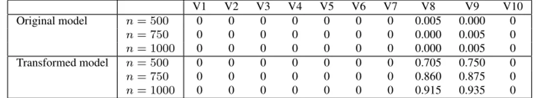
which is equivalent to model 1, but with the covariates exponentially distributed. We re-place the coefficient 5 of model 1 with 1/20 in order to have the same signal/error ratio and so to make the results comparable with those of model 1. For model (31), the hard-threshold linearity test of Lafferty and Wasserman (2008) is not consistent. For such a model, table 3 shows the percentage of times that the nonlinearity threshold is exceeded, for different values of n. The three rows on the top refer to the application of the test to the original model in (31), using the non-uniform covariatesX(j) and the basic BID procedure, for n = 500, 750, 1000 respectively. The three rows on the bottom refer to the application of the test to the transformed modelg(u) = m(F−1X (u)) obtained from (31) as explained in section 7. Note that only the covariates 8 and 9 are nonlinear. The hard-threshold nonlin-earity test misses the detection of such nonlinearities for the original model, as expected,
V1 V2 V3 V4 V5 V6 V7 V8 V9 V10 Original model n = 500 0 0 0 0 0 0 0 0.005 0.000 0 n = 750 0 0 0 0 0 0 0 0.000 0.005 0 n = 1000 0 0 0 0 0 0 0 0.000 0.005 0 Transformed model n = 500 0 0 0 0 0 0 0 0.705 0.750 0 n = 750 0 0 0 0 0 0 0 0.860 0.875 0 n = 1000 0 0 0 0 0 0 0 0.915 0.935 0
Table 3:Percentages of rejection of the linearity hypothesis in the hard-threshold test of Lafferty and Wasser-man (2008), for model (31). The rows on the top refer to the original model in (31), with non-uniform covariates X(j). The rows on the bottom refer to the transformed model, with uniform covariates ˆU(j).
while it correctly identifies the nonlinearities for the transformed model. Of course, the percentages for covariates 8th and 9th are lower than those observed in figure 2, since the transformed model is obtained by estimating the distribution function, so an additional es-timation error is involved. The other results, for the eses-timation of the bandwidths and the regression function, are equivalent to those reported in figure 2.
A. Assumptions and proofs
(A1) The bandwidthH is a diagonal and strictly positive definite matrix.
(A2) The multivariate Kernel function K(u) is a product kernel, based on a univariate kernel functionK(u) with compact support, which is non negative, symmetric and bounded; this implies that all the moments of the Kernel exist and that the odd-ordered moments ofK and K2are zero, that is
∫ ui1
1 ui22· · · uiddKl(u)d(u) = 0 if someijis odd, forl = 1, 2. (32)
(A3) The second derivatives ofm(x) are |mjj(x)| > 0, for each j = 1, . . . , k.
(A4) All derivatives ofm(·) are bounded up to and including order s.
(A5) (hU, . . . , hU) ∈ B ⊂ Rdand(hL, . . . , hL) ∈ B ⊂ RdwithhU > hL> 0. (A6) The density functionfX(x) of (X1, . . . , Xd) is Uniform on the unit cube.
Proof of Theorem 1. The first part of Theorem 1,P (hj = hU) → 1 for j > k, follows
straightforward by using Lemmas 3 and 4 and the same arguments as in the proof of Lemma 7.5 in Lafferty and Wasserman (2008).
Now, we suppose thatj ≤ k (nonlinear covariate), for which we have to estimate the optimal multivariate bandwidth. By (17) and (18) we have thatVjL= O(n−1), ∀j. More-over, by Lemma 1, there exists one and only one multivariate optimal bandwidth, say {h∗
1, . . . , h∗k}. It can be shown that h∗i = O (n−α), i = 1, . . . , k, with α > 0. But {h∗i},
i = 1, . . . , k, is the solution of the system in Lemma 1. So, we have to satisfy the following condition
O(n−5α) + O(n−5α) = O(n−1+(k−1)α).
Without loss of generality, we can writeh∗Uj = hUjn−α andh∗Lj = hLjn−α, with some hU j > hLj > 0, j = 1, . . . , k. By Lemma 3, E ( d BjU L ) = BjU L+ O(n−2α), j ≤ k.
Since the solutions of the system in Lemma 1 are continuous functions of dBjU Land cVjL, we have that ˜hj = Op(n−1/(4+k)), j = 1, . . . , k. Since P (j is nonlinear) → 1, ∀j ≤ k,
whenn → ∞, the result follows. ✷
Proof of Theorem 2. The proof follows the same lines as in Corollary 5.2 in Lafferty and
Wasserman (2008) using the results of Theorem 1. ✷
Proof of Theorem 3. LetUi := FX(Xi) := (F1(Xi(1)), . . . , Fd(Xi(d))), where Fj(·)
is the univariate marginal distribution function, j = 1, . . . , d. Let ˆUi := ˆFX(Xi) :=
( ˆ F1(Xi(1)), . . . , ˆFd(Xi(d)) ) =(Uˆi1, . . . , ˆUid )
, where ˆFj(·) is the empirical distribution
function,j = 1, . . . , d.
We use the idea of Choi et al. (2000). LetWi := ∏dj=1 h1jK
(x
j−Uij
hj
)
as in (7.21) of Lafferty and Wasserman (2008) and ˆWi:=∏dj=1h1jK
(x
j− ˆUij
hj
) .
Now we consider the first element in the matrix (7.20a) of Lafferty and Wasserman (2008). Using the Taylor’s expansion aboutUi, we have
1 n n ∑ i=1 ˆ Wi = 1 n n ∑ i=1 Wi+ 1 n n ∑ i=1 ( ˜W′ i)T( ˆUi− Ui) where ( ˜W′
i) is a d dimension vector of the first derivatives of Wi with respect to Uij,
j = 1, . . . , d evaluated in a point, say ηi, which belongs to a neighborhood ofUisuch that
∥ηi∥ ≤ ∥ ˆUi− Ui∥, with ∥ · ∥ the Euclidean norm.
Let ˆA11:= 1n∑ni=1WˆiandA11:= n1 ∑ni=1Wi. It follows that
P( ˆA11− E(A11)
> ϵsj(h)
)
≤ P (|A11− E(A11)| > ϵsj(h)/2) + (I)
+P ( 1 n n ∑ i=1 ( ˜W′ i)T( ˆUi− Ui) > ϵsj(h)/2 ) (II), where s2 j(h) = nhC2 j ∏d
i=1h1i as in Lemma 7.1 of Lafferty and Wasserman (2008). The
constantC is defined in (7.10) of Lafferty and Wasserman (2008). We put ϵ = √δ log n as in Lemma 3. For the part (I), using the proof of Lemma 7.1 in Lafferty and Wasserman (2008), we have that P (|A11− E(A11)| > ϵsj(h)/2) ≤ ( 1 n )c1
For the second expression in (II), since the dimension of vectors is finite,d, it is sufficient to bound a component of positionj, that is
1 n n ∑ i=1 ˜ W′ ij( ˆUij − Uij) ≤ sup x∈R ˆFj(x) − Fj(x) n1 n ∑ i=1 ˜W′ ij .
Since the Kernel function is defined on a compact set and its first derivative is bounded, it follows that n1 ∑ni=1
˜W′ ij
= Op(1), j = 1, . . . , d. Using the Hoeffding’s inequality we
have that P ( sup x∈R ˆFj(x) − Fj(x) > ϵsj(h) ) ≤ n−c2 j = 1, . . . , d,
where0 < c2 < ∞ and it is independent of n.
Putc := min{c1, c2}. Finally, it follows that I + II ≤ n−c. So, we have the same kind
of bound as in Lafferty and Wasserman (2008) and Lemma 3.
Using the arguments above, we can show that the other elements of the matrices in (7.20a), (7.35) and (7.39) of Lafferty and Wasserman (2008) have the same order of con-vergence as in Lemma 7.1 of Lafferty and Wasserman (2008) and Lemma 3. The results of Lemma 7.4 in Lafferty and Wasserman (2008) and Lemma 4 hold again.
Using the assumptions of this Theorem we can writem(Xi) = m · F−1X (Ui) := g(Ui).
So that, the assumption (A6) is still valid. Moreover, the arguments above show that we can use the approximationg( ˆUi). In general, when we consider a linear covariate with
Fj which is not uniform, the functiong(·) becomes non linear. In this way, we can apply
Theorem 1 withr non linear covariates. The result follows. ✷
Proof of Theorem 4. It is sufficient to apply Theorem 2 replacing Theorem 1 with Theorem
3. ✷
B. Lemmas and Corollaries
To be simple, we arrange the covariates as follows: nonlinear covariates forj = 1, . . . , k,
linear covariates for j = k + 1, . . . , r and irrelevant variables for j = r + 1, . . . , d.
Moreover, the set of linear covariatesA can be further partitioned into two disjoint subsets: the covariates fromk + 1 to k + sc belong to the subsetAc, which includes those linear
covariateswhich are multiplied to other nonlinear covariates, introducing nonlinear mixed
effectsin model (1); the covariates from k + sc + 1 to r belong to the subset Au, which
includes those linear covariates which have a linear additive relation in model (1) or which are multiplied to other linear covariates, introducing linear mixed effects in model (1). Therefore,A = Ac∪ AuandC ∪ A ∪ U = {1, . . . , d}. In such a framework, the gradient
and the Hessian matrix of the functionm become
Dm(x) = DCm(x) DAc m(x) DAu m (x) 0 Hm(x) = HCm(x) HCAc m (x) 0 0 HCAc m (x)T HAmc(x) 0 0 0 0 HAu m (x) 0 0 0 0 0 (33)
where0 is a vector or matrix with all elements equal to zero. Note that the matrices HCm(x), HAc
m(x) and HAmu(x) are symmetric, whereas the matrix HCAm c(x) is not. Moreover, for
additive models without mixed effects, all the sub-matrices in Hm(x) are zero, except for
HC
m(x), which is diagonal.
In our analysis, it is also necessary to take account of those terms in the Taylor’s expan-sion ofm(x) involving the partial derivatives of order 3 (see the proof of Lemma 2 for the details). To this end, we define the following matrix
Gm(x) = ∂3m(x) ∂x3 1 ∂3m(x) ∂x1∂x22 . . . ∂3m(x) ∂x1∂x2d ∂3m(x) ∂x2∂x21 ∂3m(x) ∂x3 2 . . . ∂3m(x) ∂x2∂x2d .. . ... . .. ... ∂3m(x) ∂xd∂x21 ∂3m(x) ∂xd∂x22 . . . ∂3m(x) ∂x3 d = GCm(x) 0 0 0 GAcC m (x) 0 0 0 0 0 0 0 0 0 0 0 . (34)
Note that the matrix Gm(x) is not symmetric. Note also that, for additive models, matrix
GAcC
m (x) is null while matrix GCm(x) is diagonal.
In the same way, let the bandwidth matrix beH = diag(HC, HAc, HAu, HU).
Remem-ber that∥HC∥ → 0 for n → ∞.
Lemma 2. Under model (1) and assumptions (A1)-(A6), withs = 5, the conditional bias
of the local linear estimator given by (4) is equal to
E ˆ m(x; H) ˆ DC m(x; H) ˆ DAc m(x; H) ˆ DAu m (x; H) ˆ DU m(x; H) − m(x) DCm(x) DAc m (x) DAu m (x) 0 X1, . . . , Xn = Bm(x, HC) + Op ( n−1/2), where Bm(x, HC) = 1 2µ2 tr{HCm(x)H2C} + ν1(H4C) GCm(x)H2 C1 + ( µ4 3µ2 2 − 1 ) diag{GCm(x)H2C}1 + ν2(H4C) GAcC m (x)H2C1 + ν3(H 4 C) 0 0 ,
where the functionsν1(·) : Rk→ R, ν2(·) : Rk → Rkandν3(·) : Rk→ Rsc are such that
ν1(0) = 0, ν2(0) = 0 and ν2(0) = 0.
Proof: In general, we follow the classic approach used in Ruppert and Wand (1994) and Lu (1996), a part from one substantial difference, i.e. we do not assume that the bandwidths tend to zero for n → ∞. This implies that we must bound all the terms of the Taylor expansion with respect tom(x) and with respect to fX(x), given that the size of the interval
around the pointx does not vanish with n → ∞. Anyway, assumption (A6) imply that the Taylor expansion is exact with respect tofX. This simplifies remarkably the proof.
The conditional bias of the LLE is given by
E( ˆβ(x; H)|X1, . . . , Xn) − β(x) = (ΓTW Γ)−1ΓTW(M − Γ β(x))
whereM = (m(X1), . . . , m(Xn)) and, given ut= H−1(Xt− x), we have Sn = 1 n n ∑ t=1 ( 1 uTt ut utuTt ) |H|−1K(ut) Rn = 1 n n ∑ t=1 ( 1 ut )[ m(Xt) − m(x) − DTm(x)Hut]|H|−1K(ut).
ForSn, using Taylor’s expansion and assumptions(A2) and (A6), we have
Sn = ∫ ( 1 uT u uuT ) K(u)fX(x + Hu)du + Op(n−1/2) = ∫ ( 1 uT u uuT ) K(u) + Op(n−1/2) = ( 1 0 0 µ2Id ) + Op(n−1/2). (36)
For the analysis ofRn, we need to introduce some further notation. Suppose that the
functionm(x) has at least up to order 3 continuous partial derivatives in an open neighbor-hood ofx = (x1, . . . , xd)T. Let define thekth-order differential Dmk(x; y) as
Dkm(x, y) = ∑ i1,...,id k! i1! × . . . × id! ∂km(x) ∂xi1 1 . . . ∂xidd yi1 1 × . . . × yidd,
where the summation is over all distinct nonnegative integersi1, . . . , idsuch thati1+ . . . +
id= k. Using the Taylor’s expansion to approximate the function m(Xt), and assumption
(A6), we can write Rn = 1 n n ∑ t=1 ( 1 ut ) [ 1 2!D 2 m(x, Hut) + 1 3!D 3 m(x, Hut) ] |H|−1K(ut) + R∗n = ∫ ( 1 u ) [ 1 2!D 2 m(x, Hu) + 1 3!D 3 m(x, Hu) ] K(u)fX(x + Hu)du + R∗n + Op(n−1/2) = ∫ ( 1 u ) [ 1 2!D 2 m(x, Hu) + 1 3!D 3 m(x, Hu) ] K(u)du + R∗n+ Op(n−1/2) whereR∗
n represents the residual term, which depends on higher order derivatives of the
functionm(x). Now, given assumption (A2), some of the terms in the k-th order differen-tials cancel. We have
Rn = ∫ ( 1 2!D2m(x, Hu) 1 3!uD3m(x, Hu) ) K(u)du + R∗n+ Op(n−1/2) = ( r1+ r1∗ r2+ r∗2 ) + Op(n−1/2), (37)
where the termsr∗
1andr∗2comes fromR∗n. Solving the integrals and applying the properties
of the Kernel function we have r1 = ∫ 1 2D 2 m(x, Hu)K(u)du = 1 2 d ∑ i=1 d ∑ j=1 ∂2m(x) ∂xi∂xj hihj ∫ uiujK(u)du = 1 2µ2 k ∑ i=1 ∂2m(x) ∂xi∂xi h2i = 1 2µ2tr{H C m(x)H2C};
in the same way, the element of positionj of the vector r2is r2(j) = ∫ 1 6urD 3 m(x, Hu)K(u)du = ∑ i1,...,id hi1 1 · · · hidd i1! × . . . × id! ∂3m(x) ∂xi1 1 · · · ∂x id d ∫ ui1 1 · · · uirr+1· · · uiddK(u)du = ∑ s̸=r 1 2µ 2 2 ∂3m(x) ∂xr∂x2s hrh2s+ 1 6µ4 ∂3m(x) ∂x3 r h3r , while the whole vectorr2is equal to
r2= 1 2µ 2 2 [ HGm(x)H2+ ( µ4 3µ2 2 − 1 ) diag{HGm(x)H2} ] 1. Following the same arguments, it is easy to show thatr∗
1 = ν1(H4C). Combining the (35), (36) and (37), we obtain E( ˆβ(x; H)|X1, . . . , Xn) − β(x) = diag{1, H−1}S−1n Rn = ( r1+ r∗1 1 µ2H −1(r 2+ r∗2) ) + Op(n−1/2) ≈ ( 1 2µ2tr(HCmH2C) + ν1(H4C) 1 2µ2GmH21 + ( µ4 6µ2 − 1 2µ2 ) diag(GmH2)1 + µ12H−1r∗2 ) .
The result follows after some algebra and splitting the last row in four components,C, Ac,
AuandU , respectively. ✷
Corollary 1. Under the assumptions (A1)-(A6), withs = 5, the conditional asymptotic
bias and the asymptotic variance of the partial derivative estimators ˆD(j)m(x; H), defined in
(4), are Abias{ˆD(j) m (x; H)} = ν4(H2C), Avar{ˆD(j)m(x; H)} = σ2 ερ2 n|H|h2 j forj ∈ C ∪ AC, withν4(·) : Rk→ R, ν4(0) = 0 and
Abias{ˆD(j)m(x; H)} = 0, Avar{ˆD(j)m(x; H)} = σ 2 ερ2 n|H|h2 j forj ∈ C ∪ AC .
Proof: It is a direct consequence of Lemma 2, using (33) and (34). In fact, using
assump-tions (A1)-(A6), withs = 5, the asymptotic conditional covariance matrix is
Cov ˆ DC m(x; H) ˆ DAc m(x; H) ˆ DAu m (x; H) ˆ DUm(x; H) X1, .., Xn = σ 2 ερ2 n|H| H−2C 0 0 0 0 H−2A c 0 0 0 0 H−2A u 0 0 0 0 H−2U (1+op(1)).
✷
Proof of Lemma 1. Definedj :=
BU L
j
(hU)2−(hL)2, Aj(h) := ∑i̸=jk dih2i andVj := VjLhL,
j = 1, . . . , k. In this way we can rewrite the equations of Lemma 1 as 4d2jh5j+ 4Aj
(
h(0))djh3j− Vj = 0, j = 1, . . . , k,
for some initial vector h(0). Fix aj. It is easy to verify that the function fj(hj) := 4d2jh5j+
4Aj
( h(0)
)
djh3j − Vj has one and only one real positive solution, that is h(1)j such that
fj(h(1)j ) = 0. Considering j ∈ {1, . . . , k}, we can build the vector h(1)with the elements
h(1)j , given the vector h(0). So, there exist continuously differentiable functions, gj, such
thath(v)j = gj(h(v−1)), j = 1, . . . , k, v ∈ N. Now, using Dini’s Theorem, we have
∂h(v)j ∂h(v−1)i = −2dih(v−1)i h (v) j 5dj(h(v)j )2+ 3Aj(h(v−1)) i ̸= j. Note that ∂h (v) j ∂h(v−1)i
= 0 for i = j. But, for increasing values of v ∈ N, {h(v)} forms a sequence in a compact space of Rk, sayS. So, we can extract a subsequence from {h(v)} which is convergent inS, that is limn→∞h(vn) = h∗ ∈ S, with vn→ ∞ when n → ∞.
Without loss of generality, we can consider S = {h : ∥h∥ = 1} where ∥ · ∥ is the Euclidean norm. Consider thesign(x) function, equal to 1 for positive x and to -1 for negativex. If sign(djAj(·)) > 0 then 5dj(h(v)j )2+ 3Aj(h(v−1)) has a minimum at h(v)j =
0. It follows that k ∑ i=1 ∂h(v)j ∂h(v−1)i h (v−1) i = −2h(v)j Aj(h(v−1)) 5dj(h(v)j )2+ 3Aj(h(v−1)) ≤ 2 3.
Ifsign(djAj(·)) < 0, using h(v)j >√−3Aj(·)/(5dj), we obtain k ∑ i=1 ∂h(v)j ∂h(v−1)i h (v−1) i = −2h(v)j Aj(h(v−1)) 5dj(h(v)j )2+ 3Aj(h(v−1)) > 0 ∀v.
So, in this case,{h(v)j } is a monotone sequence with respect to v. Since limn→∞h(vj n) =
h∗
j, a component of the vector h∗, it follows thatlimv→∞h(v)j = h∗j. Using these
argu-ments, we can conclude that there exists one and only one solution, h∗. ✷
We have to state some technical lemmas to prove the Theorems 1 and 2. First of all, we introduce the following quantities. Consider a vector h = (h1, . . . , hk). Let q(h) :=
∑k
j=1pjh2j andq(h; yi) :=∑kj̸=ipjh2j + piyi2, for somek < d and 0 < pj < ∞, ∀j. Let
Rt(K) :=
∫
K(u)K(wtu)du, with w0= 1 and w1 = hL/hU. Define
s21(hU) := 1 n(hU)dσ 2 ϵR0(K), s22(hU; hL) := s21(hU)/w1, s23(hU; hL) := s21(hU) R1(K) R0(K) .
Lemma 3. For every hU = (hU, . . . , hU) ∈ B and hL = (hL, . . . , hL) ∈ B, vectors of
dimensiond, if the assumptions (A1)-(A6) hold, with s = 4, then
E ( d BU L j ) = BU L j + O ( q(hU)(hU)2− q(hU; hL)(hL)2) j ≤ k, E ( d BU L j ) = 0 j > k. Moreover,∀δ > 0 P d BU L j − E ( d BU L j ) sB(hU; hL) >√δ log n ≤ 2n−δσ 2 ϵ/(16c2),
wheres2B(hU; hL) := s21(hU) + s22(hU; hL) − 2s23(hU; hL) and c2 := max{c21; c22} with
c21 := s21(hU)/s2B(hU; hL) and c22:= s22(hU; hL)/s2B(hU; hL).
Proof of Lemma 3. Using the assumptions and Lemma (7.1) in Lafferty and Wasserman (2008),E
( d BjU L
)
can be easily derived. Note thatpjin the quantitiesq(hU) and q(hU; hL)
depend on the fourth order derivatives of the functionm(·). Now, we can write
d BjU L− E ( d BjU L ) sB(hU; hL) = = mˆ ( x; HU)− E(mˆ (x; HU)) s1(hU) c1− ˆ m(x; HLj)− E(mˆ (x; HLj)) s2(hU; hL) c2.
So, we have that
P d BjU L− E ( d BjU L ) sB(hU; hL) >√δ log n ≤ P ( ˆ m(x; HU)− E(mˆ (x; HU)) s1(hU) > √ δ log n 4c2 1 ) + +P ˆ m(x; HL j ) − E(mˆ (x; HL j )) s2(hU; hLj) > √ δ log n 4c22 .
Using the Bernstein’s inequality as in the proof of Lemma 7.1 in Lafferty and Wasserman
(2008), the result follows. ✷
Now we consider the estimator in (27), forj = 1, . . . , d, as c
Lemma 4. For every hU = (hU, . . . , hU) ∈ B and hL = (hL, . . . , hL) ∈ B, vectors of
dimensiond, if the assumptions (A1)-(A6) hold, with s = 4, then ∀ϵ > 0
P c VL j s22(hU; hL) − 1 > ϵ → 0 n → ∞.
Proof of Lemma 4. The result follows by means of Theorem 2.1 in Ruppert and Wand (1994) and Lemma 7.4 in Lafferty and Wasserman (2008). It is sufficient to use Lemma 7.4 in Lafferty and Wasserman (2008) without taking the derivative with respect to the
bandwidthhj. ✷
References
Bertin, K. and Lecué, G. (2008) Selection of variables and dimension reduction in high-dimensional non-parametric regression, Electronic Journal of Statistics, 2, 1224–1241. Choi, B., Hall, P. and Rousson, V. (2000) Data sharpening methods for bias reduction in
nonparametric regression, The Annals of Statistics, 28, 1339–1355.
Comminges, L. and Dalalyan, A.S. (2012) Tight conditions for consistency of variable selection in the context of high dimensionality, The Annals of Statistics, 40, 2667–2696. Dai, Y. and Ma, S. (2012) Variable selection for semiparametric regression models with
iterated penalisation, J. of Nonparametric Statistics, 24, 283–298.
Fan, J. and Gijbels, I. (1995) Data-driven bandwidth selection in local polynomial fitting: variable bandwidth and spatial adaptation, J. of the R. Statistical Society, series B, 57, 371–394.
Györfi, L., Kohler, M., Krzyzak, A. and Walk, H. (2002) A Distribution-Free Theory of
Nonparametric Regression, Springer-Verlag, Heidelberg.
Lafferty, J. and Wasserman, L. (2008) Rodeo: sparse, greedy nonparametric regression,
The Annals of Statistics, 36, 28–63.
La Rocca, M. and Perna, C. (2005) Variable selection in neural network regression mod-els with dependent data: a subsampling approach, Computational Statistics and Data
Analysis, 48, 415–429.
Li, R. and Liang, H. (2008) Variable selection in semiparametric regression modeling,
The Annals of Statistics, 36, 261–286.
Lin, L. and Lin, F. (2008) Stable and bias-corrected estimation for nonparametric regres-sion models, J. of Nonparametric Statistics, 20, 283–303.
Lin, B. and Zhang, H. (2006) Component selection and smoothing in multivariate non-parametric regression, The Annals of Statistics, 34, 2272–2297.
Lu, Z. (1996) Multivariate locally weighted polynomial fitting and partial derivative esti-mation, Journal of Multivariate Analysis, 59, 187–205.
Ruppert, D. (1997) Empirical-bias bandwidths for local polynomial nonparametric regres-sion and density estimation, J. of the American Statistical Association, 92, 1049–1062.
Ruppert, D. and Wand, P. (1994) Multivariate locally weighted least squares regression,
The Annals of Statistics, 22, 1346–1370.
Storlie, C., Bondell, H., Reich, B. and Zhang, H. (2011) Surface estimation, variable selection, and the nonparametric oracle property, Statistica Sinica, 21, 679–705. Variyath, A., Chen, J. and Abraham, B. (2010) Empirical likelihood based variable
selection, J. of Statistical Planning and Inference, 140, 971–981.
Yang, L. and Tschernig, R. (1999) Multivariate bandwidth selection for local linear regression, J. of the Royal Statistical Society, Series B, 61, 793–815.
Zhang, H., Cheng, G. and Liu, Y. (2011) Linear or nonlinear? automatic structure discovery for partially linear models, J. of the American Statistical Association, 106, 1099–1112.