Hierarchical latent variable models for dimensionality reduction: an application on composite indicators

(1)

sionality reduction: an application on

com-posite indicators

Scuola di Scienze Statistiche

Dottorato di Ricerca in Statistica Metodologica – XXXII Ciclo

Candidate Carlo Cavicchia ID number 1348873

Thesis Advisor Prof. Maurizio Vichi

(2)

in front of a Board of Examiners composed by:

Prof. Roberto Rocci Prof. Bruno Toaldo Prof. Simone Vantini

Hierarchical latent variable models for dimensionality reduction: an application on composite indicators

Ph.D. thesis. Sapienza – University of Rome

This thesis has been typeset by LA_{TEX and the Sapthesis class.}

Version: February 17, 2020

(3)

(4)

(5)

Acknowledgments

I never expected to start a Ph.D. but the last three years have been the most intense and powerful experience of my life. Most importantly, I have never been alone. I am grateful to all my colleagues and the professors of the Department of Statistical Sciences who have been extraordinarily important for me. Let me just cite two wonderful girls who made these last years special, Tullia and Silvia. Since you have introduced me in Stanza 41, you have been more than simple friends. The list of all the people who contributed to make my Ph.D. experience so great is too long, so I can simply thank each and all of you.

Since my Bachelor’s degree, I was guided and supported by Prof. Maurizio Vichi. I would like to express all my gratitude to you for everything you did for me, both as an academic advisor and a man: you fully contributed to my personal growth.

This thesis is a collection of different works developed throughout these years. I therefore want to wholeheartedly thank who collaborated with me, namely Prof. Pasquale Sarnac-chiaro for all his support and help, and my colleague and friend Giorgia, for always putting up with me.

Amongst my lifetime friends, I pick just two special guys who supported me day by day, Luca and Alessio. Thank you for all the moments together and for pushing me into the craziest thing of my life: ASD Valcanneto Futsal.

I would like to dedicate not only this thesis but also all my Ph.D. to my parents, Susanna and Antonio, for giving me your best every single day. Even if what I do is not clear yet, you always work in order to guarantee my well being. Matteo, this work is also for you, for having inspired my life from the very start.

I should thank too many people who contributed to make me who I am now, especially in these last three years. So then again, simply a heartfelt thanks to all of you.

(6)

(7)

List of Figures

1.1 Hierarchical CI. This is the graphical representation considered in the

Struc-tural Equation Modeling . . . 4

1.2 Reflective and Formative Models . . . 5

1.3 Example of Reflective construct . . . 6

1.4 Example of Formative construct . . . 7

2.1 An example of heatmap of Rx . . . 24

2.2 Heatmaps of examples of correlation matrix produced by the simulation study with different levels of error. . . 26

3.1 Heatmap of 3 data matrices X with (left) small, (center) medium and (right) large errors. . . 43

3.2 Heatmap of matrix X formed by 3 blocks of variables. . . 44

3.3 Two-Levels Models for CI . . . 46

3.4 Comparison among empirical distribution of variances. . . 48

4.1 Path diagram of two-levels hierarchy . . . 66

4.2 Normalized scores of Eu Countries: A) RCE, B) GW, C) PII and D) WM . 68 5.1 Relationship between a (2H − 1)-ultrametric correlation matrix and a corre-sponding hierarchy of latent concepts. . . 77

5.2 Comparison between heat maps of observed and estimated correlation matrices. 81 5.3 Aggregation of latent concepts in Benchtoldt hierarchical structure. . . 81

(10)

(11)

List of Tables

2.1 Simulated datasets with n = 200, J = 20, H = 5 and different levels of error. 26 2.2 Simulated datasets with n = 200, J = 50, H = 10 and different levels of error. 27 2.3 Percentage of times Cronbach’s alpha (computed for each cluster of MIs)

> 0.9 with different scenario and different levels of error. . . 27

2.4 Percentage of times Cronbach’s alpha (computed for each cluster of MIs) < 0.7 with different scenario and different levels of error. . . 27

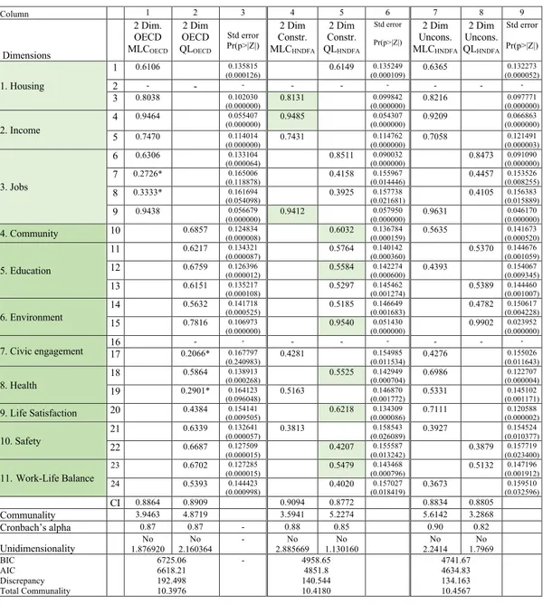
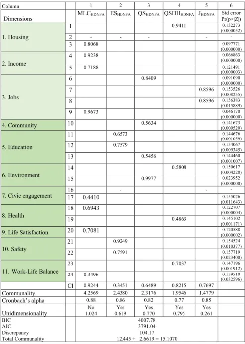
2.5 Analysis of different hierarchical two level factor analysis models for defin-ing two dimensions of well-bedefin-ing: material livdefin-ing conditions and quality of life. . . 31

2.6 Analysis of different hierarchical two level factor analysis models for defin-ing five dimensions of well-bedefin-ing. . . 33

3.1 Types of normalizations . . . 47

4.1 List of MIs. . . 63

4.2 List of countries. . . 64

4.3 Results of the optimal model for defining dimensions of waste management. 65 4.4 Rankings based on SCIs and GCI according to these thresholds, green: normalized score > 0.60, yellow: normalized score > 0.30 and < 0.60, red: normalized score < 0.30 . . . 67

4.5 Spearman’s correlations among SCIs and with WM . . . 67

5.1 Simulation study results. . . 80

(12)

(13)

Abstract

This thesis is devoted to the development of new hierarchical latent variable models for Dimensionality Reductionwith a specific focus on the construction of Composite Indicators (CIs). Since our society is producing a huge quantity of data, the construction of model-based CIs represents an interesting and still open methodological challenge. This dissertation is motivated by the necessity to provide model-based CIs which are built according to a statisticalapproach avoiding subjective choices (e.g., normative weights), therefore, the new insights and proposals hope to represent a contribution to the current literature. This thesis provides an introduction to CIs, a brief review of the most used methods in Multidimensional Data Analysis framework, a discussion about measurement models and methodological proposals to model latent concepts. Factor Analysis and its hierarchical extensions have been introduced in order to set the starting point of the analysis. A first proposal represents a new latent factor model that could be used for building CIs, it aims to investigate the hierarchical structure of the data in order to define two levels of CIs. The model, named Hierarchical Disjoint Non-Negative Factor Analysis is composed of two novelties: a model which is the two level hierarchical extension of FA and its disjoint extension with non-negative loadings. The latter model is enriched by considerations about the CIs used for tracking coherent pol-icy conclusions. A set of features, properties and rules useful to build "good" CIs have been presented and explained. The last proposal in the thesis represents a new model for positive data correlation matrices which aims to detect reliable concepts and to build the hierarchy from them to the most general one. The proposed models are illustrated both via simulation studies and real data applications, to analyze their performances and abilities. In particular, the main application in this thesis regards the construction of a hierarchically aggregated index for the multidimensional phenomenon Waste Management in European Union. Waste Managementis becoming even more important for its impact on human-being’s lives, and many data have been produced about it, therefore the construction of a CI able to reduce its dimensionality and to highlight the main dimensions of it has a extraordinary usefulness in order to provide support to EU countries’ action and policies.

Acknowledgments

A special thank goes to the reviewers, Marco Fattore and Andrea Cerioli, for their precious comments and feedback.

(14)

(15)

Chapter 1

Introduction

1.1 Introduction

In the last years, with the data revolution and the use of new technologies, phenomena are frequently described by a huge quantity of information useful for making strategic decisions. A priority for policymakers is having simple statistical tools useful to synthesize data. Such tools are represented by Composite Indicators (CIs). In policy-making, it is important underline that CIs should never be meant as a goal per se, they are starting points for public interest discussion and they detect the trend of the phenomenon under study.

According to OECD Glossary of Statistical terms, a Composite Indicator (CI) is formed when individual indicators (i.e., manifest or observed variables) are compiled into a single non-observable index, on the basis of an underlying model for the multidimensional concept that is being measured. Multidimensional concepts are also defined as latent constructs, like well-being (Stiglitz, Sen, and Fitoussi 2009), development, poverty, environmental conditions, etc., which cannot be adequately captured by a single observed indicator, and a set of individual indicators is needed. A CI, for the JRC - Composite Indicator Research Group (JRC-COIN)1, is a mathematical combination, or aggregation (weighting), of the manifest indicators (MIs) that generally have different unit of measurement and can be differently combined (Nardo, Saisana, Saltelli, Tarantola, et al. 2005; OECD-JRC 2008). CIs are easier to interpret than trying to find a common trend in many separated indicators. Therefore, CIs are increasingly used for bench-marking countries’ performances and the methodological challenges raise a series of technical issues that, if not adequately addressed, can lead to CIs being misinterpreted or manipulated. Yet doubts are often raised about the robustness of the resulting countries’ rankings and about the significance of the associated policy message. According to Nardo, Saisana, Saltelli, and Tarantola (2005), arguments in favour of CIs are that they: summarise complex multi-dimensional phenomena in view of supporting decision-makers; provide an overall picture of the separate indicators thus simplifying the interpretation; facilitate the task of ranking countries on complex issues; attract public interest by providing a summary figure to use for assessing performances; reduce the size of a list of indicators. Whereas, contrary arguments are that CIs: may send misleading

1_{The Joint Research Centre (JRC) is the European Commission’s science and knowledge service which} employs scientists to carry out research in order to provide independent scientific advice and support to EU policy. The JRC is a Directorate-General of the European Commission under the responsibility of Tibor Navracsics, Commissioner for Education, Culture, Youth Sport.

(16)

and/or non-robust policy messages if they are poorly constructed or misinterpreted, and thus, they may invite politicians to draw simplistic policy conclusions; may involve subjective decisions in the CI construction phase that can influence the final indicator. Even if the issue of the construction of composite indicators has been discussed many times by many authors with different approaches, CIs do not have a good reputation because the statistical methods used are not always mathematically rigorous and often they are based on theories which do not seem to have a solid foundation (Mazziotta and Pareto 2013). Often CIs are computed as the weighted mean of the MIs (e.g., Multidimensional Poverty Index, Alkire and Foster (2011), Alkire, Foster, et al. (2015), and UNDP (2018)), where the weights represent the importance of each MI and they are chosen by the researcher subjectively or according to a known theory (i.e., normative weights). In particular, many authors do not appreciate CIs determined by subjective weights on the MIs because it can lead to misinterpretation of the results (Nardo, Saisana, Saltelli, and Tarantola 2005; Saltelli et al. 2004).

The definition of CI includes the notions of concept and model that need additional clarifications. The concept in the CI can be measured only indirectly and it relates to a fact, in general to a phenomenon of interest that, for its nature, cannot be sufficiently described by a single MI2. This is a typical situation in multivariate statistics, where the simultaneous observations and analysis of more than one indicator is needed to understand the phenomenon being studied. Concepts such as for example poverty, human development, gender equality, well-being cannot be satisfactorily represented by individual indicators and therefore need to be described by several indicators. The model is the second notion considered to characterize a CI. It is required to simplify and synthesize the complexity of the reality by means of a mathematically-formalized reconstruction of the observed data and their main relations. Models are needed for investigating phenomena in order to achieve awareness driven by the empirical evidence. In the development process used to specify the appropriate CI model for the studied phenomenon, three integral parts are needed: the variable selection, to properly characterize the phenomenon under study, the model selection from a set of candidate models and the model evaluation to assess the performances of the CI.

In order to evaluate and/or confirm the quality of building approach, even when CIs are built as average of MIs as it is the case of Human Development Index (HDI, (Alkire 2010)) and MPI, the researcher needs a set of properties able to test the CI’s capacity of reconstructing the manifest data or its ability of forming the studied concept. It is important to notice how the choices of the researcher might affect the result of the analysis. The use of a modeling approach, including selection and assessment, guarantees the researcher who wishes to construct the CI based on a scientific method, to build it on a body of techniques with desirable properties to guarantee that the CI will work appropriately in different conditions and with past and future data.

Our society is producing a huge quantity of data in every moment, a model-based approach able to reduce the dimensionality of data has a crucial applicability and an extraor-dinary usefulness. The methodological challenges of constructing well-done CIs in order to acquire new knowledge based on empirical evidence is even more important. Models are crucial in the development process used to specify the appropriate CI for the studied

2_{A MI is a variable that indicates something, thus it should provide information about the phenomenon,} otherwise it might be meant as a simple statistic. If a concept has only one dimension with one indicator, the concept is practically equivalent to a variable.

(17)

phenomenon.

The use of a model-based CI classifies this approach as statistical because hypotheses formulated in the specification of the CI are empirically tested. The methodology wishes to be objective and transparent, avoiding - as far as possible - the use of arbitrary choices that cannot be tested.

In this thesis, we suppose that the model for CIs is a Dimensionality Reduction (DR) model with a hierarchical structure that goes from the original MIs to the final General Composite Indicator (GCI), passing through a reduced set of Specific Composite Indicators (SCIs), i.e., dimensions, which measure specific concepts describing the main components of the phenomenon under study. CIs are usually computed starting from a reduced number of MIs (e.g., MPI and HDI) whereas it is more and more necessary to have tools able to handle a large number of MIs. The proposal should be considered into the Dimensionality Reductionframework for its capacity of compiling big quantity of information into a single CI, by way of many steps of aggregation.

The process of Dimensionality Reduction produce, for sure, a loss of information and the presentation of the single CI without additional information may denote a too simple picture of the complex phenomenon that it synthesizes. Indeed, the goal of the analysis is to show all the process of reduction, that is, the MIs (e.g., scoreboard, portfolio of variables) used to describe the phenomenon, the SCIs illustrating their synthesized dimensions and representing the most relevant components of the phenomenon, and the final GCI. Together with these information, it is useful to show the entire hierarchical process that goes from the MIs to the GCI, that is, the relationships, internal to the indicators (manifest or composite) used to describe the phenomenon. In addition, it would be necessary to add at each step of the reduction a model fit or measures of reliability and unidimensionality that allow the researcher to assess if the model correctly describes and synthesizes the data. In this way, the researchers have all the information at hand and can decide the most appropriate level of description to use for their purposes. For example, to measure the dimensions of well-being is appropriate to stop the analysis at the SCIs’ level such as Material Living Conditions and Quality of Life(Stiglitz, Sen, and Fitoussi 2009).

Thus, in this thesis we will study methodologies of Dimensionality Reduction to build model-based CIs, underlying a body of properties and features that a good CI should respect in order to avoid poorly constructed indexes that induce simplistic and misleading policy conclusions. This thesis is framed in Latent variable models context because it refers to indicators (i.e., latent) that are not directly observable but they affect the manifest ones.

1.2 Hierarchical structure

CIs usually have a hierarchical structure, in fact, they identify a multidimensional concept that summarizes other multidimensional concepts, each one characterized by other nested multidimensional concepts or by subsets of MIs. For example, the CI of well-being defined in the Better Life Initiative of OECD (2001) is seen as a mathematical combination of Material Living Conditions (MLC) and Quality of Life (QL). The MLC is certainly a multidimensional concept characterized by housing, jobs and income. QL is the second multidimensional concept described by community, education, safety, health, environment, civic engagements, life satisfaction and work-life balance. Each one of these last dimensions of the well-being are also multidimensional concepts described by several indicators or by

(18)

Figure 1.1. Hierarchical CI. This is the graphical representation considered in the Structural Equation Modeling

other multidimensional concepts. For example, heath can be described by child health and reproductive health. A field of study where the hierarchical approach is used to model and build CIs is psychometrics. For instance, hierarchical models have been used frequently in the cognitive domain (J. Carroll 1993; Horn and Cattell 1966; Horn and Cattell 1982); in the personality domain (Cattell 1957; Cattell 1966; Eysenck and Himmelweit 1947; Eysenck 1967; DeYoung, Peterson, and Higgins 2002; Digman 1997), and for modeling anxiety (R.E. Zinbarg and Barlow 1996; R.E. Zinbarg, Barlow, and Brown 1997).

It is worth to observe that these examples refer to the definition of Latent variable models, the aim is representing individual characteristics that cannot be directly observed (e.g., well-being, quality of life, personality, intelligence, etc.).

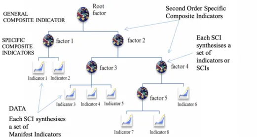
In general, the initial set of MIs is aggregated into classes (i.e., sets, clusters), each one representing a multidimensional concept summarised by a theoretical indicator, also named latent variable or factor. MIs within classes are supposed highly correlated so that the common information can be summarised by factors. Classes of measured indicators are continuously aggregated and represented by new factors until when all initial MIs are together into a single class and represented by a general factor that corresponds to the CI. In other terms, data useful to accurately describe the studied phenomenon are “best” reconstructed at different levels of syntheses by means of DR, considering some Specific Composite Indicators as representative of subsets of MIs. The process of reduction has a hierarchically nested form, as shown in Figure 1.1, with a graphical configuration of a tree. Leaves represent the MIs, while internal nodes denote SCIs (i.e., latent variables, factors, linear or non-linear combinations of MIs) that synthesize common information in the data. In order to represent CIs and their hierarchies, the path diagram (i.e. tree graph) is usually used: the GCI is at the top of the graph, as root of the tree and the leaves are the MIs. MIs are described by rectangles, while SCIs or GCI are represented by circles, which are seen as latent factors corresponding to theoretical concepts.

The aim of the analysis is the definition of nested latent concepts from the MIs to the GCI in order to reconstruct the hierarchical structure of the data correlation matrix. In the

(19)

GCI SCI1 SCI2 Ω2 Ω1 Ω3 _Ω 5 Ω4 Ω6

(a) Fully reflective model for CI; i.e, SCI1→ (Ω1, Ω2, Ω3, SCI2→ (Ω4, Ω5, Ω6), GCI → (SCI1, SCI2).

GCI SCI1 SCI2 Ω2 Ω1 Ω3 _Ω 5 Ω4 Ω6

(b) Partially reflective model and partially formative model for CI; i.e, SCI1→ (Ω1, Ω2, Ω3, SCI2→ (Ω4, Ω5, Ω6), GCI → SCI1, SCI2→ GCI.

Figure 1.2. Reflective and Formative Models

simplest case, a two-levels structure is hypothesised taking into account only the levels of SCIs and the GCI, however when we are interested to investigate about all the possible aggregations from SCIs level to the root of the hierarchy it is possible to detect all the intermediate concepts via an ultrametric correlation matrix.

1.3 Measurement Models and Multidimensional Data Analysis

Measurement modelsrefer to the implicit or explicit models that relate the latent variable to its MIs (Bollen 2001). Two different approaches might be distinguished with respect to the nature of the relationships between MIs and latent constructs (i.e., SCIs and GCI) which formally describe the measurement model, and thus, define the direction of the these relationships (Blalock 1964; Bollen and Bauldry 2011).

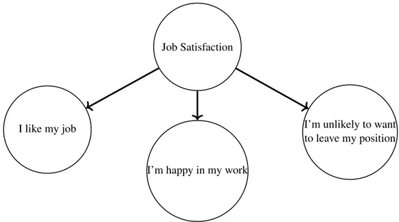
An arrow starting from a CI and pointing to a MI describes a casual relationship from CI to MI (CI → MI). In other terms, the CI reconstructs (predicts, explains) the MIs. The relation of the type CI → MI is called reflective, i.e., the CI explains the correlation among MIs contributing to specify the concept associated with the CI. Blalock (1964) referred to this kind of indicators as effect indicators. This is the typical relation in Factor Analysis (FA, (T. Anderson and Rubin 1956; Horst 1965)) where a set of latent variables is used to reconstruct the MIs. So, latent constructs are determinant of the MIs, it is a top-down approach. In Figure 1.2(a) a fully reflective GCI is specified with two SCIs. If a SCI is pointing to a set of MIs it means that the concept corresponding to the SCI reconstructs the common variance of the MIs. On the arrow, a loading (i.e., weight) is generally reported which generally represents the correlation between SCI and MI. The example in Figure 1.3 can help the reader to understand the reflective relation.

The relation of the type MI → CI is formative and describes a causal relation from MI to CI. Blalock (1964) explained this kind of relation saying that the MIs influence the latent variable rather than the reverse, and some refer to these as formative indicators or casualindicators. A formative relation can also have the form SCI → GCI from SCI to GCI. Indicators (MIs or SCIs) that form a concept with a formative relation generally are not correlated to each other. This is the typical relation in multiple and multivariate regression. In this case the links between MIs and contructs are measured through a bottom-up approach. In Figure 1.2(b), a GCI in part reflective and in part formative is shown. It is important

(20)

Job Satisfaction

I like my job

I’m happy in my work

I’m unlikely to want to leave my position

Figure 1.3. Example of Reflective construct

to highlight that an entirely formative model is not identified (Edwards 2011), such that without additional information it is impossible to find unique values for the parameters in the model and hence cannot assess indicator validity (Bollen 2011). In order to solve this problem, the alternative model named MIMIC has been considered (Hauser and Goldberger 1971; Jöreskog and Goldberger 1975) by taking into account the latent variable as effect of some MIs and, at the same time, cause of some others. Edwards (2011) proposed a critique about formative models by arguing that formative measures are often based on expressed beliefs about constructs and MIs that do not respect condition of unidimensionality and reliability, and that are difficult to defend.

The CI may reconstruct other CIs in the hierarchy (SCI1→ SCI2). In this case, a second

order or in general a higher order SCI is used. Also, in this case the weight on the arrow representing the formative relation corresponds to the correlation between the involved indicators. An example can help the reader to understand the formative relation (see Figure 1.4).

So, in a reflective relation, MIs depend on the latent indicators (i.e. SCIs); whereas in a formative relation, MIs affect the latent indicators (i.e. SCIs).

Within the methodological literature, the discussion between reflective and formative is crucial and far from a possible solution. Reflective indicators are appropriate for many situations in psychological measurement, but they are not appropriate for all situations. Several authors (Blalock 1964; Land 1970; Bollen 1984; Bollen 1989; Bollen and Lennox 1991; Hayduk 1987; MacCallum and Browne 1993) have underlined that some MIs should be, for their nature, more appropriately treated as casual rather than effects of the latent construct. It is important to remark that the choice between the two kinds of model should not depend directly on the researcher, but it should depend exclusively on the nature of the phenomenon and its definition (Diamantopoulos and Siguaw 2006; Maggino 2017). Moreover, it is not possible to test a priori the nature of the phenomenon in order to establish if it is reflective or formative (Maggino and Zumbo 2012). Often researchers do not consider that a latent indicator may be causal and treat all MIs as effect indicators. This is not an

(21)

Job Satisfaction

Good pay

Good boss

Work hours are ideal

Figure 1.4. Example of Formative construct

inconsequential decision since causal and effect indicators have different properties and their incorrect classification can bias estimates from a model (Bollen and Lennox 1991). In order to better understand the difference between the two aforementioned approaches of the measurement model, see Jarvis, MacKenzie, and Podsakoff (2003) and Edwards and R.P. Bagozzi (2000).

In other cases, the indicators of a psychological construct might be a mixture of effect and causal indicators. For instance, as reported by Bollen and Ting (2000), Bollen and Lennox (1991) had considered that the Center for Epidemiological Studies Depression Scale (CES-D; Radloff (1977)) has some effect indicators (e.g., "I felt depressed" and "I felt sad") and some causal indicators (e.g., "I felt lonely").

Another situation is considered by Cavicchia, Vichi, and Zaccaria (2020a), the hierar-chical aggregations of MIs start as reflective and become formative at a certain level of the hierarchy itself. Thus, the type of the latent constructs definition changes at first level where no correlation exists among constructs (the correlations are tested according to Chen, Zhang, and Zhong (2010)). This consideration can be explained by saying that until correlations between latent constructs are statistically significant, the latent constructs reflect the same upper latent concepts, when the correlations stop being statistically significant, the latent constructs form the upper latent concepts.

The hierarchical path model associated with the process to define the CI highlights the different levels of description of the phenomenon associated with the CI can be derived, starting from MIs (scoreboard) and considering one or more sets of SCIs to arrive to the final GCI. All the hierarchy is given; thus, the researcher will have the possibility to use only the scoreboards reorganized according to the given model, or additionally will consider the different levels of reduction given by the SCIs and the GCI.

Formally, the CI is a model-based indicator if the CI assumes a statistical model of the type

X = CIM+ E (1.1)

(22)

the matrix of the MIs reconstructed by the CI model, and E is the residual, that is, the difference between X and CIM. E corresponds to the part of data not explained by the

CI model and generally, it includes the measurement error (i.e., a random error, sampling bias) always present in the measurement of the MIs. When the model-based CI is used, it can be estimated by considering an estimation method which minimizes a badness-of-fit or discrepancy function, i.e., a function of the difference between the MIs and the fitted CI (i.e., predicted MIs).

Multidimensional Data Analysis (MDA) approaches, like FA or Principal Component Analysis (PCA) (Pearson 1901; Hotelling 1933), are considered valid in order to build CIs for multidimensional phenomena. In PCA and FA, the weights are computed by taking into account the statistical relations among MIs. They represent reflective models thus they can be used whether all the indicators refer to a general latent concept. Another widely used methods for the construction of CIs are Structural Equation Modeling (SEM) (Jöreskog 1970; Bollen 1989; Kaplan 2000), they are used in order to build a flexible system of composite indicators able to model causal relations among them. Trinchera and Russolillo (2010) provided a useful review on the use of SEM to build CIs.

In OECD (2004) and OECD-JRC (2008), the FA is considered as a weighting method in order to combine MIs. FA has the advantage to define loadings that best reconstruct the MIs according to the estimation method chosen avoiding the subjective choice of a system of weights by the researcher. However, some choices are needed, for instance the choice of type of rotation (varimax, equimax, orthomax, etc.) (Browne 2001) and the size of the soft threshold3. The concept of oblique (i.e., non-orthogonal) factors in order to get more interpretable simple structure has been subject of study of many authors (Cattell and Khanna 1977; Harman 1976; Jennrich and Sampson 1966; Clarkson and Jennrich 1988). Specifically, strategies have been proposed to rotate factors so as to best represent "clusters" of MIs, without the constraint of orthogonality of factors. However, the oblique factors produced by such rotations are often not easily interpreted.

When the model presents a hierarchical structure, FA is not an appropriate method because it is neither able to get a partition of the MIs nor to get the hierarchical structure of the concepts, therefore a valid alternative method to construct a CI into the factor analysis framework is the Hierarchical Confirmatory Factor Analysis (HCFA, Holzinger (1944), Jöreskog (1966), Jöreskog (1969), Jöreskog (1978), and Jöreskog (1979)), which can be used by first theorizing the correlation structure between factors and the related MIs. However, the prior knowledge on both the number factors and the most relevant relations between MIs and factors represents a limitation in the construction of the CI in the situation, quite realistic, when the researcher has not an exact theory in mind or when the theory demonstrates to be erroneous in some parts or at least in its empirical application. Hierarchical Factor Analysis (HFA) strategy, proposed by Thompson (1951) and Schmid and Leiman (1957), and detailed by Wherry (1959), Wherry (1975), and Wherry (1984), first identifies clusters of MIs and rotates axes through those clusters; next it computes the correlation matrix of the SCIs (oblique factors). The correlation matrix of oblique factors is further factor-analyzed to yield a set of orthogonal factors that divide the variability in the MIs into that due to shared or common variance (secondary factors), and unique variance due to the clusters of similar MIs

3_{Soft thresholding is a raw solution to improve interpretability. It consists of ignoring MIs with} small-magnitude loadings, and therefore, each factor is approximated by a linear combination of only a subset of MIs, namely those with not small-magnitude loadings. This is also named "Truncated Factor Analysis". The size of the threshold is subjective.

(23)

in the analysis (primary factors). Also Le Dien and Pages (2003) proposed a hierarchical extension of multiple factor analysis (Escofier and Pages 1998), called Hierarchical Multiple Factor Analysis, which aims to provide graphical displays of the MIs groups for each level of the hierarchy or superimposed representations of partial individuals.

The distinction between confirmatory and exploratory approach is explained in the context of FA to highlight the difference between Confirmatory FA and Exploratory FA by Ullman (2006).

In this situation, the researcher can assume that each manifest indicator is mainly related with a latent construct only, although this relation is not assumed known a priori. In this case an unknown Simple Structure Model (SSM) is hypothesised for the data.

In recent years several methods have been proposed in order to provide a clearer in-terpretation of the factors (or components) by means of a sparse structure of the loading matrix, i.e., assuming that some loadings are equal to zero (d’Aspremont et al. 2007; Gr-bovic, Dance, and Vucetic 2012; Jolliffe, Trendafilov, and Uddin 2003; Zou, Hastie, and Tibshirani 2006; Ferrara, Martella, and Vichi 2016; Ferrara, Martella, and Vichi 2018). Ferrara, Martella, and Vichi (2016) proposed a constrained PCA called Disjoint Principal Component Analysis(DPCA), as particular case of Clustering Disjoint Principal Compo-nent Analysis(Vichi and Saporta 2009), which allows to identify the sparsest classification of variables via principal components with maximum variance, summarising information held by the corresponding subset of variables. Whereas, Disjoint Factor Analysis (DFA) (Vichi 2017) has been proposed to identify the best SSM for the data in FA framework. Maximum Likelihood Estimation (MLE) of DFA allows to make inference on the number of factors, on the relations between MIs and factors (loadings), and to assess the validity of the SSM for the observed data. In addition, DFA allows to identify the eventual presence of relevant cross-loadings (Vichi 2017) and hence, identify multi-factor indicators, that tend to complicate the naming and interpretation of factors. Finally, DFA permits to fix one or more indicators that must specify the same factor. This allows the researcher to hypothesise even a part of a theory that he/she has in mind and believes is important to be included in the model in order to be successively confirmed.

However, DFA is not appropriate to identify the hierarchical structure of factors. This is so because DFA assumes that factors are orthogonal and therefore it is not supposed observable a hierarchical structure of factors and it is not hypothesised that factors are mutually related and share some common information that can be summarised by the general indicator through reflective relationships. The aggregation of uncorrelated factors is own of formative models.

In order to solve this problem, it is assumed that correlation structure in the data has a hierarchical form, albeit unknown, with at least two levels; the first denoted root or general level, representing the CI and at least a single specific level indicating a reduced set of multidimensional concepts described by disjoint classes of MIs. In this thesis we will concentrate on the two level hierarchical structure which is generally the most proposed in CFA. Thus, it is supposed that the model for CIs is a Dimensionality Reduction model with a hierarchical structure that goes from the original MIs to the final General Composite Indicator (GCI), passing through a reduced set of Specific Composite Indicators (SCIs), which are dimensions that measure specific concepts describing the main components of the phenomenon taken into study.

(24)

1.4 Non-aggregative approach

Although this dissertation hinges on a specific reflective hierarchical approach to build CIs which characterizes the general CI as a weighted sum of factor scores (i.e. aggregative approach), in the interests of providing a complete introduction of CIs, a brief description of the non-aggregative approach is presented in this Section.

Rankings, which are very common, cannot be aggregated through linear combinations, averages or other functionals, designed for numerical variables. Therefore, in order to treat ordinal attributes as numerical, before aggregation they are often transformed into numerical scores, through more or less sophisticated scaling tools (Fattore 2017). However Madden (2010) showed evidence that such procedures may lead to controversial results and questioned whether it is correct to force concepts which are naturally conceived in ordinal terms into numerical settings. In the non-aggregative approach, thus, the synthesis should not be conducted through a weighted sum of MIs and, in general, it should not involve any explicit function of them. Consequently, the need for properly managing rankings has led to the development of modern tools and methodologies into the framework of partial order theory to prioritize observations by many different ordinal characteristics (Brüggemann and Patil 2011).

Partial order theory has been considered a fundamental branch of mathematics, only of theoretical interest, for a long time. However, in the last years, its effectiveness as a tool for data analysis is being increasingly realized and many applications of partially ordered sets to real problems in statistics and applied sciences have appeared, hence demonstrating their insightfulness and usefulness. Main examples pertain to the analysis of complex and multidimensional systems of ordinal data and to problems of multi-criteria decision making, both extremely relevant in socio-economic and environmental sciences (Brüggemann and Patil 2011; Fattore and Maggino 2014).

Following the definition in (Davey and Priestley 2002), a partially ordered set (or a POSET) P = (X , <) is a set X (called the ground set) equipped with a partial order relation <, that is, a binary relation satisfying the properties of reflexivity, antisymmetry and transitivity. Let v1, . . . , vkbe k ordinal evaluation variables, profiles (each possible sequence of scores

on v1, . . . , vk) can be (partially) ordered in a natural way by a given dominance criterion.

Poset tools, thus, allow to describe and to exploit the relational structure of the data, so as to compute evaluation scores in purely ordinal terms and avoiding any aggregation of variables. Since ordinal phenomena cannot be measured against an absolute scale, the evaluation scores to be assigned to the profiles are computed comparing them against some reference profiles selected as benchmarks.

Eventually, the evaluation is addressed in terms of multidimensional comparisons among profiles rather than through attribute score aggregations. In other words, the central idea in partial order is comparison, and the most general outcome is a net of relations between observations according to their indicator values, respecting the ranking aim (Carlsen and Brüggemann 2013). This makes it not needed to scale ordinal attributes into numerical variables, overcoming the issues of aggregative procedures and counting approaches. The evaluation procedure is fuzzy by nature, and it accounts for both vagueness and intensity of deprivation, thus producing a comprehensive set of synthetic indicators for policy-makers (Fattore 2016).

From this moment onwards, we will focus on hierarchical latent variable models for Dimensionality Reduction, as this thesis presents hierarchical factorial models to build CIs.

(25)

1.5 Chapter Summaries

Chapter 2 presents a new latent factor model that could be used for modeling CIs named Hierarchical Disjoint Non-Negative Factor Analysis(HDNFA). The proposal is grounded on the common definition of latent variable model and it is an exploratory methodology to model the hierarchical structure of factors, which is supposed in part or totally unknown, identifying a reduced set of factors (i.e., SCIs) each one related to a disjoint subset of MIs. Each subset of MIs must be internally consistent and reliable, that is, MIs are concordant with the related SCI and loadings must be positive. Properties are discussed for HDNFA. Furthermore, an application to optimally identify the dimensions of well-being is used to illustrate the characteristics of the model. The proposed model has been implemented in a MATLAB routine.

The contents of Chapter 2 have been developed with Prof. Maurizio Vichi, and are reported in a paper which has been submitted for publication and it is currently under first revision in a international journal, see Cavicchia and Vichi (2020a).

Chapter 3 introduces a model-based approach for construction of CIs as an alternative method of estimation for the model HDNFA, and a body of properties and features that a good CI shoud have. In order to assess some well-know CI such as HDI and MPI, a comparison with the proposed model-based CI based on the same properties has been presented. Chapter 3 provides useful tools for studying CIs which are of interest in many applicative fields.

The contents of Chapter 3 have been developed with Prof. Maurizio Vichi, and are reported in a paper which has been submitted for publication and it is currently under second revision in a international journal, see Cavicchia and Vichi (2020b).

Chapter 4 presents a hierarchical CI for Waste Management in Europe by using the HDFNA model. The model has detected three main reliable aspects of the phenomenon of interest. The analysis, from the MIs selection to the definition of the CI, represents an application of the model presented in Chapter 2 and it has a crucial importance for supporting policy-making. Waste Management is increasing its importance through the years and the number of statistics dedicated to it is getting larger and larger. The construction of a CI which highlights the main aspects of it has been a interesting challenge with the aim to provide support to EU countries’ action and policies.

The contents of Chapter 4 have been developed with Prof. Pasquale Sarnacchiaro and Prof. Maurizio Vichi, and are reported in a paper which has been submitted for publication and it is currently under first revision in a international journal, see Cavicchia, Sarnacchiaro, and Vichi (2020).

Chapter 5 introduces a novelty model that aims to reconstruct the data correlation matrix through an ultrametric correlation matrix which is able to pinpoint the hierarchical nature of the phenomenon under study. The model is able to detect consistent latent concepts and the relationship among them starting their correlation structure, as well as it provides a measure for the internal consistency of concepts and a measure for the correlation among concepts. An application on Bechtoldt dataset is proposed to show the performance of the model. The proposed model has been implemented in a MATLAB routine.

The contents of Chapter 5 have been developed with Prof. Maurizio Vichi and Dr. Giorgia Zaccaria, and are reported in a paper which has been submitted for publication and it is currently under second revision in a international journal, see Cavicchia, Vichi, and Zaccaria (2020b).

(26)

(27)

Chapter 2

Hierarchical Disjoint Non-Negative

Factor Analysis

2.1 Introduction

Hierarchical Disjoint Non-Negative Factor Analysis(HDNFA) is a new latent factor model that could be used for modeling Composite Indicators (CIs). CIs, in general, are multidi-mensional concepts described by at least a theoretical construct (i.e., factor) which is related to a cluster of MIs. Frequently CIs have a hierarchical structure, i.e., they are characterized by a set of specific factors (i.e., SCIs, dimensions) each one corresponding to disjoint, or nested clusters of MIs. Hierarchical Confirmatory Non-Negative Factor Analysis can be used to assess the hierarchical structure of the CIs. Hierarchical Disjoint Factor Analysis is grounded on the common definition of a latent variable model and it is presented as an exploratory methodology to model the hierarchical structure of factors, which is supposed in part or totally unknown, identifying a reduced set of factors each one related to a disjoint cluster of MIs.

Furthermore, in a definition of a CI, each cluster of MIs (i.e., measured variables, observed variables) must be internally consistent and reliable, that is, MIs related to the factor measure “consistently” a unique theoretical construct. This implies that MIs are concordant with the related factor and loadings must be positive. This last requirement is included as a constraint in the new methodology that for this reason is named Hierarchical Disjoint Non-Negative Factor Analysis.

Properties are discussed for HDNFA. The model and its algorithm has also the option to constraint a MI to load on a pre-specified factor in order to hypothesize, a priori, some relations between MIs and factors that the researcher wishes to fix. An application to optimally identify the dimensions of well-being is used to illustrate the characteristics of the new methodology. A final discussion completes the paper.

The paper is organised as follows. two level Hierarchical Factor Analysis (HFA) model is proposed in Section 2.2. Section 2.3 includes an overview of disjoint models. Section 2.4 introduces the non-negative constraints of the factors necessary to specify consistent latent indicators. A simulation study is considered in Section 2.5. Section 2.6 shows an application of the HNDFA. A final discussion completes the paper in Section 2.7.

It is important to underline that, in this paper, latent constructs are computed as factors, thus the term "factors" and "composite indicators" (i.e., SCIs and GCI) are used with the

(28)

same meaning.

2.2 Two level Hierarchical Factor Analysis

Let x be the (J × 1) random vector, representing the generic multivariate observation, with mean vector µx= [µ1, . . . , µJ]0, and J-dimensional variance-covariance matrix Σx. The two

level Hierarchical Factor Analysis is a new factorial model that considers two typologies of latent unknown constructs: H specific factors and a single (nested) general factor identified by the two simultaneous models (equations)

x − µx= Ay + ex (2.1)

y = cg + ey (2.2)

where A is the (J × H) matrix of unknown specific factors loadings and ex is a (J × 1)

random vector of errors.

It is assumed that y ∼ NH(0, Σy) where Σyis the correlation matrix of the specific factors,

and ex∼ NJ(0, Ψx), where cov(ex) = Ψxis the J dimensional diagonal positive definite

variance-covariance matrix of the error of model 2.1 and cov(ex, y) = Σyex= 0.

Furthermore, g is the random general factor with mean 0 and variance σ_g2= 1, denoting the composite indicator related to a reduced set of specific factors and c is the (H × 1) vector of unknown general factor loadings. In addition, eyis a non-observable (H × 1) random

vector of errors. It is assumed that g ∼ N(0, 1) and ey∼ NH(0, Ψy), where cov(ey) = Ψy

is the H-dimensional diagonal positive definite variance-covariance matrix of the error of model 2.2. In addition it is assumed that errors in the two models are uncorrelated cov(ex, ey) = Σeyex = 0; and errors and factors are uncorrelated, i.e., cov(ey, g) = Σeyg= 0.

Model 2.1 identifies H specific theoretical constructs by means of a common factor model that identifies common information with H factors related to the MIs; while model 2.2 detects the general theoretic construct (the composite indicator) by means of a one-factor model that identifies common information with one general factor related to the H specific factors. Given these assumptions and including model 2.2 into model 2.1 the two level Hierarchical Factor Analysis model is defined

x − µx= A(cg + ey) + ex= Acg + Aey+ ex (2.3)

from which it can be derived that x ∼ NJ(µx, Σx), where the variance-covariance matrix Σx

is

Σx= cov(Acg + Aey+ ex)

= Accov(g)c0A0+ Acov(ey)A0+ cov(ex)

= Acc0A0+ AΨyA0+ Ψx

= AΣyA0+ Ψx (2.4)

with

Σy= cc0+ Ψy (2.5)

Matrix Σy is a correlation matrix since specific factors are standardized. Similarly to

(29)

relations between MIs and factors. Model 2.4 is a restricted Confirmatory Factor Analysis model, that is an oblique common factor model, where Σyhas the form Σy= cc0+ Ψy.

Many hierarchical extensions of FA have been proposed by many authors through the years (e.g., Thompson (1951), Schmid and Leiman (1957), Wherry (1959), Wherry (1975), Wherry (1984), and Le Dien and Pages (2003)); the novelty of the proposal consists of the covariance structure given by the model (2.4 and 2.5). Although the proposal has developed as two nested models: first order factors model (2.1) and second order factor model (2.2), all parameters of the model (2.3) are estimated simultaneously via a descent coordinate algorithm (Section 2.2.2).

Property 1. A necessary but not sufficient condition for the HFA model identification is that the number of unknown parameters must be smaller or equal to the number of equations

JH+ 2H + J ≤J(J + 1)

2 (2.6)

where JH, H, H, J, parameters are in A, c, Ψy and Ψx, respectively. In fact, for the

estimation of model parameters in HFA the number of equations must be larger than or equal to the number of parameters. The equations of the HFA model are J(J+1)₂ , while JH+ 2H + J are the number of parameters.

Property 2. Given H and Ψxthe parametersA, c, Ψyare not unique.

To see this, let matrixZ be any non-singular matrix of order H such that

A∗= AZ (2.7) Σ∗_y= Z−1ΣyZ0−1= c∗c0∗+ Ψ∗y (2.8) with c∗= Z−1c (2.9) e∗_y= Z−1ey (2.10) cov(e∗_y) = Ψ∗_y= Z−1cov(ey)Z0−1= Z−1ΨyZ0−1 (2.11) thus A∗Σ∗_yA0∗+ Ψx= AZZ−1ΣyZ0−1Z0A0+ Ψx= AΣyA0+ Ψx (2.12)

This illustrated a fundamental indeterminacy in the Hierarchical Factor Analysis model similar to EFA. In fact,

x − µx= A∗c∗g + A∗e∗y+ ex

= AZ−1Zcg + AZ−1Zey+ ex

= Acg + Aey+ ex (2.13)

Therefore, without further restrictions the model parametersA, c, Ψy are not uniquely

identified. This indeterminacy will be used to require that the total variance of the factors in model (2.13) is maximized.

(30)

2.2.1 Maximum Likelihood estimation of the two level Hierarchical Factor Analysis model

Suppose that a random sample of n > J multivariate observations xi= [xi1, . . . , xiJ]0, i =

1, . . . , n of x is observed; thus, the log-likelihood is L(xi,µx, A, c, Ψx, Ψy) = = −nJ 2 log(2π) − n 2log |A(cc 0_{+ Ψ} y)A0+ Ψx| − 1 2 n

∑

i=1 (xi− µx)0Σ−1x (xi− µx) (2.14)

Maximizing L with respect to µxgives the sample mean; thus rewriting

∑ni=1(xi−bµx)

0

Σ−1_x (xi−µbx) = nS yields to the reduced log-likelihood L(xi,A, c, Ψx, Ψy) = = −nJ 2 log(2π) − n 2{log |A(cc 0 + Ψy)A0+ Ψx| + tr[(A(cc0+ Ψy)A0+ Ψx)−1S]} (2.15) It is worth to note that the maximization of L(xi, A, c, Ψx, Ψy) is equivalent to the

minimization of the discrepancy function D(xi,A, c, Ψx, Ψy) =

= log |A(cc0+ Ψy)A0+ Ψx| − log |S| − J + tr{[A(cc0+ Ψy)A0+ Ψx]−1S} → min A,c,Ψx,Ψy

(2.16) Let S, Ψx, Ψybe positive definite matrices, Ψx, Ψydiagonal and c real (H × 1) vector.

The minimization of the discrepancy function (2.16) is equivalent to the minimization of the function

f = log |A(cc0+ Ψy)A0+ Ψx| + tr{[A(cc0+ Ψy)A0+ Ψx]−1S} (2.17)

Define Σx= A(cc0+ Ψy)A0+ Ψxand C = Σ−1x − Σ−1x SΣ−1x , by differentiating function

f with respect to A gives ∂ f /∂ A = 2tr(A0C)∂ A.

Thus, the first-order condition is CA = 0, or equivalently A = SΣ−1_x A, which corresponds to require Σx= S. Therefore, A(cc0+ Ψy)A0= S − Ψx = Ψ 1 2 x(Ψ −1 2 x SΨ −1 2 x − I)Ψ 1 2 x = Ψ 1 2 x(TΛT0− I)Ψ 1 2 x = Ψ 1 2 xT(Λ − I)T0Ψ 1 2 x (2.18) where Ψ− 1 2 x SΨ −1 2

x = TΛT0 is a spectral decomposition, with T orthonormal eigenvectors

and Λ the diagonal matrix of eigenvalues. Thus, A(cc0+ Ψy) 1 2 = Ψ 1 2 xT(Λ − I) 1 2 (2.19)

(31)

and therefore A = Ψ 1 2 xT(Λ − I) 1 2(cc0+ Ψ_y)− 1 2 (2.20)

Differentiating f with respect to Ψxgives ∂ f /∂ Ψx= trC∂ Ψx. Since Ψxis diagonal

and since the first-order condition for A is S = Σx, thus the first-order condition for Ψxis

diag(S) = diag(Σx), hence

diag(S) = diag(A(cc0+ Ψy)A0+ Ψx) (2.21)

Therefore,

Ψx= diag(S − (A(cc0+ Ψy)A0) (2.22)

To compute c also the first-order conditions for A have to be satisfied cc0= A+(S − Ψx)A0+− Ψy = Ψ 1 2 y(Ψ −1 2 y (A+(S − Ψx)A0+)Ψ −1 2 y − I)Ψ 1 2 y = Ψ 1 2 y(ULU0− I)Ψ 1 2 y = Ψ 1 2 yU(L − I)U0Ψ 1 2 y (2.23) where Ψ− 1 2 y (A+(S − Ψx)A0+)Ψ −1 2

y = ULU0 is a spectral decomposition with U orthonormal

eigenvectors, L the diagonal matrix of eigenvalues and A+is the Moore-Penrose pseudoin-verse of A (i.e., A+= (A0A)−1A0). Note that matrix A0A is diagonal, so its inverse is easy to compute. Thus, c = Ψ 1 2 yU(L − I) 1 2 _(2.24)

To compute Ψythe first order conditions for Ψxhave to be satisfied

diag(A+(S − Ψx)A0+) = diag(cc0+ Ψy) (2.25)

Therefore,

Ψy= diag(A+(S − Ψx)A0+− cc0) (2.26)

In the next section, the five steps of the algorithm of HFA are summarized.

2.2.2 Algorithm of HFA

Given H, a coordinate descent algorithm for the estimation of the model (2.3) can be described by five steps which are sequentially repeated until a stopping rule is satisfied. Step 0 [Initialization] Fix the matrix bΨΨΨx= diag(S), then the algorithm starts by computing

b A = bΨΨΨ 1 2 xT(Λ − I) 1

2, where T and Λ are eigenvectors and eigenvalues of b_Ψ_Ψ_Ψ

−1 2 x S bΨΨΨ −1 2 x ;

then compute bΨΨΨy= diag(bA+(S − ΨΨΨx)bA0+).

Step 1 Given bΨΨΨx,bA and bΨΨΨythe minimization of the discrepancy function (2.16) with respect

to c is given by (2.24).

Step 2 Given bΨΨΨx,bA andbc the minimization of the discrepancy function (2.16) with respect to Ψ

Ψ

(32)

Step 3 Compute ΣΣΣy=bcbc

0_{+ b}

ΨΨΨy, then transform covariances in correlations.

Step 4 Given bΨΨΨx, bΨΨΨyandbc the minimization of the discrepancy function (2.16) with respect to A is given by (2.20).

Step 5 Given bA, bΨΨΨyandbc the minimization of the discrepancy function (2.16) with respect to ΨΨΨxis given by (2.22).

The five Steps 1, 2, 3, 4 and 5 are alternated repeatedly. At each step the discrepancy function decreases or at least does not increase. If the reduction of the discrepancy is larger than an arbitrary small positive constant the algorithm continues to iterate, otherwise the algorithm stops and is considered to have converged to a solution that is not guaranteed to be the global minimum. However, repeating the analysis from different random starts, it is observed that in our experiments the solutions are always the same. As shown in Property 2, the solution of HFA is not unique, so it is necessary to include some constraints.

2.2.3 Maximization of the explained variance

Given H, let bΨx, bA, bΨy and =bc the maximum estimates of the model (2.3); thus, the estimated variance-covariance matrix is:

b

Σx= bA(bcbc

0

+ bΨy)bA0+ bΨx (2.27)

As shown by Property (2) the MLE solution (2.27) is not unique, thus a non-singular matrix Z can be defined

A∗= bAZ (2.28)

Ψ∗_y= Z−1Ψb_yZ0−1 (2.29)

c∗= Z−1bc (2.30)

such that minimizes

||_(H)bΣx− bAZZ0Ab0||2= ||_(H)bΣ

1 2

x− bAZ||2 (2.31)

where(H)bΣx= P(H)L(H)P0(H)is the rank-H approximation from the spectral decomposition

of the matrix bΣx and the columns of P(H) are H eigenvectors, whereas the values on the

diagonal of L(H)the corresponding H eigenvalues of the matrix bΣx.

From the solution ZZ0= bA+_(H)Σb_xAb0+, matrix Z is derived

Z = bA+P_(H)L

1 2

(H) (2.32)

Now, tr((H)Σbx) is the total variance that can be explained by a rank-H approximation

of bΣx. Since tr((H)bΣ_x) = ||_(H)bΣ

1 2

x − bAZ||2+ ||bAZ||2, by minimizing (2.31) is equivalent to

maximize the variance ||A∗||2_{explained by the H-dimensional solution of HFA.}

Therefore, the indeterminacy can be positively used to find among the infinite solutions the one that most explains the variance reconstructed by the H-dimensional solution of

(33)

the HFA. However, this solution can still be rotated if together with the transformations (2.28,2.29 and 2.30) also a rotation is applied, that is

A∗= bAZM (2.33)

Ψ∗_y= M0Z−1Ψb_yZ0−1M (2.34)

c∗= M0Z−1bc (2.35)

where MM0= I. Varimax rotation is suggested to improve interpretation of results (Kaiser 1958; Sherin 1966; J.M.F. ten Berge 1984; J.M.F ten Berge, Knol, and Kiers 1988; Thurstone 1947).

2.3 Disjoint models

2.3.1 Disjoint Non-Orthogonal Factor Analysis

The Disjoint Orthogonal Factor Analysis (DFA) (Vichi 2017) assumes that observations can be reconstructed by a non-observable (H × 1) random vector y denoting a reduced set of (H ≤ J) common factors by considering the following model

x − µx= Ay + exX = YV0B + EX (2.36)

with

Σx= AΣyA0+ Ψx (2.37)

where, here, factors are correlated, and the loading matrix A is restricted to the product

A = BV (2.38)

where V = [vjh] is a (J × H) binary and row stochastic matrix identifying a partition of

MIs into H clusters corresponding to H factors, with vjh= 1, if the MI j-th belongs to the

h-th cluster; vjh= 0 otherwise; whereas, B = diag(b1, . . . , bJ) is a (J × J) diagonal matrix

weighting MI j-th such that

b2_j > 0 (2.39)

If it is allowed b2_j≥ 0, when b2

j = 0 the DFA admits a model selection feature, that is,

an MI is assigned to a cluster with a loading equal to zero. In this case MI j is essentially discarded from the model. DFA assumes orthogonal factors, that is, Σy= IH, however in

this paper this condition is relaxed in order to allow a hierarchical structure of the data. Thus, the DFA model can be rewritten as follows

x − µx= BVy + ex (2.40) with Σx= BVΣyV0B + Ψx (2.41) subject to constraints V = [vjh∈ {0, 1} : j = 1, ..., J, h = 1, ..., H] (2.42) V1H= 1J i.e. H

∑

h=1 vjq= 1 j= 1, ..., J (2.43) B = diag(b1, . . . , bJ (2.44) V0BBV = diag(a2_·1, . . . , a2·H) (2.45)

(34)

If Σy= IH (Disjoint Orthogonal Factor Analysis) the variance-covariance Σxis block diagonal Σx= blkdiag(Σ11, . . . , Σhh, . . . , ΣHH) =            Σ11 0 . . . 0 0 Σ22 0 . . . 0 .. . 0 . .. 0 ... 0 .. . ... 0 Σhh 0 0 .. . ... ... 0 . .. 0 0 0 0 0 0 ΣHH            (2.46)

where each block is the variance-covariance matrix Σhhof the MIs relating to the factor h,

Σhh= Bh(1nh1 0 nh)Bh+ Ψh= bhb 0 h+ Ψh (2.47) and Bh= diag(bh),bh= [b1h, . . . , bnhh] 0_{and Ψ} h= diag(ψh),ψh= [ψ1h, . . . , ψnhh] 0_{; where n} h

is the number of MIs related to the latent factor h.

Therefore, the DFA model assumes that a relevant correlation between MIs related to the same latent factor is observed and a zero, or at least a negligible, correlation between MIs each one related to a different latent factor is detected.

If Σyhas non-diagonal elements different from zero, (Disjoint Non-Orthogonal Factor

Analysis) the block diagonal variance-covariance disappears and Σxhas the form

Σx=      Σ11 Σ12 . . . Σ1H Σ21 Σ22 . . . Σ2H .. . ... Σhh ... ΣH1 ΣH2 . . . ΣHH      (2.48)

where the generic correlation between two clusters of MIs are constrained in the Σhk= Bh(1nh1

0

nk)Bk= rhkbhb

0

k (2.49)

and rhk is the correlation between factor h and factor k.

It is important to observe that in order to identify two distinct factors h and k with associated two disjoint clusters of MIs defining matrices Σhh and Σkk, high correlation

within these matrices and lower correlation within Σhkneeds to be observed. In fact, if also

highly correlation is observed in Σhkthus a single factor is present in the data since the two

clusters of MIs are not distinct and actually form a single cluster in which MIs are all highly correlated. Thus, (2.49) guarantees that correlations in Σhkare lower than correlations within

Σhhand Σkk.

2.3.2 Hierarchical Disjoint Factor Analysis

If in the HFA some a priori substantive knowledge is incorporated in the form of restrictions on the loading matrix, this usually improves the description of the latent factors and leads to a parsimonious model with a simple loading matrix structure. Therefore, if in HFA a Simple Structure Model (SSM) is assumed observed for the data, this means that the factor loading matrix has the form A = BV and the HFA model becomes the Hierarchical Disjoint Factor Analysismodel

(35)

It can be derived that x ∼ NJ(µx, Σx) with

Σx= BVΣyV0B + Ψx (2.51)

where

Σy= cc0+ Ψy (2.52)

The discrepancy function (2.16) can be rewritten D(xi, B, V, c, Ψx, Ψy) =

= log |BV(cc0+ Ψy)V0B + Ψx| − log |S| − J + tr{[BV(cc0+ Ψy)V0B + Ψx]−1S} → min B,V,c,Ψx,Ψy

(2.53)

2.3.3 HDFA Algorithm

Given H, a coordinate descent algorithm for the estimation of the model (2.50) can be described by five steps which are sequentially repeated until a stopping rule is satisfied. Step 0 [Initialization] A random partition bV is generated from a multinomial distribution in

Hcategories each one with equal probability, where categories are not empty. Matrix b

Ψ Ψ

Ψx= diag(S).

Step 1 Given bV = [v·1, . . . , v·H] for each column h = 1, . . . , H compute the rank-1

approxima-tion of the positive semi-definite matrix bΨΨΨ

−1 2 xh ShΨΨΨb −1 2 xh ∼= λ1hu1hu01h, where λ1h is the

largest eigenvalue and u1his the associated eigenvector of the variance-covariance

matrix bΨΨΨ −1 2 xh ShΨΨΨb −1 2

xh corresponding to MIs identified by v·h, the h-th column of bV.

Thus, the discrepancy function D(B, V, c, ΨΨΨx, ΨΨΨy) (2.53) is minimized with respect to

Bh= diag(bh) by b bh= bΨΨΨ −1 2 xh u1h(λ1h− 1) 1 2 _h_{= 1, . . . , H} _(2.54)

Step 2 Given bA = bBbV,bc and bΨΨΨythe minimization of the discrepancy function (2.53) with respect to ΨΨΨxis given by b Ψ ΨΨx= diag(S − bA(bcbc 0 + bΨΨΨy)bA0) (2.55)

Step 3 Given bA = bBbV, bΨΨΨxand bΨΨΨythe minimization of the discrepancy function (2.53) with

respect to c is given by bc = bΨΨΨ 1 2 yU(L − I) 1 2 (2.56)

as already seen in (2.24), where bΨΨΨ

−1 2

y (bA+(S − bΨΨΨx)bA0+) bΨΨΨ

−1 2

y = ULU0is the spectral

decomposition with U orthonormal eigenvectors and L is the diagonal matrix of eigenvalues.

Step 4 Given bA = bBbV,bc and bΨΨΨxthe minimization of the discrepancy function (2.53) with respect to ΨΨΨyis given by

b

ΨΨΨy= diag(bA+(S − bΨΨΨx)bA0+−bcbc

(36)

Step 5 Partition bV = [bv·1, . . . ,bv·H] is obtained row by row by assigning each MI j-th to the cluster h-th that most decreases the discrepancy function (2.53). Thus, formally

   b vjh= 1 if arg min h=1,...,H D(bB, [bv1·, ...,bvj·= ih·, ...,bvJ·] 0_, b c, bΨΨΨx, bΨΨΨy) b vjh= 0 otherwise (2.58)

where ih·is the h-th column of the identity matrix of order H. Note that the update of

each row of V induces the update of the loadings of the two clusters of MIs that are eventually changed.

The five Steps 1, 2, 3, 4 and 5 are alternated repeatedly. At each step the discrepancy function decreases or at least does not increase. If the reduction of the discrepancy is larger than an arbitrary small positive constant the algorithm continues to iterate, otherwise the algorithm stops and is considered to have converged to a solution that is not guaranteed to be global minimum. To avoid the well-known sensitivity of the coordinate descent algorithms to the starting values and to increase the chance of finding the global minimum, the algorithm should be run several times starting from different initial estimates of V and retaining the best solution. The algorithm generally stops after a few iterations (in our experiments and simulation studies less than 15).

Until this moment the problem of indeterminacy in the HFA has been presented by taking into account only the non-unique identification of the parameters. It has been shown in Property 2 and it has been positively used in Section 2.2.3. Therefore, showing that different estimations of the parameters can produce the same covariance structure of the model.

It is important to remark that, for fixed bA and bΨΨΨx, factor scores can be estimated by

considering different approaches. The same estimated covariance structure, thus, may correspond to infinite distinct potential factor scores (Bollen 1989; Schönemann 1973; Schönemann and Steiger 1978). This problem, referred to as factor scores indeterminacy, has been a source of considerable controversy ever since.

Many methods to estimate the factor scores have been proposed throughout the years. For instance, we consider the weighted least square estimation of E(X|Y)

b Y = X( bΨΨΨ −1 x A(bb A0( bΨΨΨ −1 x A)b −1) (2.59)

as proposed by Bartlett (1937), or simply the Thompson (1934) regression estimator b

Y = X(S−1A)b (2.60)

The problem of factor scores indeterminacy can be resumed saying that an individual in the analysis with a high ranking according to one set of factor scores, could receive a low ranking according to another set of factor scores, when both sets are consistent with the pattern of estimated coefficients. Therefore, it is worth observing that the debates surrounding factor scores indeterminacy have been harsh and with diverging opinions (Bartholomew 1981; Guttman 1955; Maraun 1996; McDonald 1974; S. Mulaik 2009; S. Mulaik and McDonald 1977; Rozeboom 1996; Wilson 1996); however, these will not be source for further discussion here.

(37)

2.4 Hierarchical Disjoint Non-Negative Factor Analysis

Let us recall that the discrepancy function (2.53) is minimized with respect to Bh= diag(bh)

by b bh= bΨ −1 2 xh u1h(λ1h− 1) 1 2 h= 1, . . . , H (2.61)

where λ1his the largest eigenvalue and u1h is the associated eigenvector of the

variance-covariance matrix bΨ− 1 2 xh ShΨb −1 2

xh corresponding to MIs identified by v·h, the h-th column of bV.

Values λ1hand u1hminimize || bΨ−

1 2 xh ShΨb −1 2 xh − λ1hu1hu 0 1h||2, or equivalently ||XhΨb −1 2 xh − p λ1hyhu01h||2 (2.62)

where Xhis the centred data matrix formed by MIs identified by v·h and yh is the factor

score vector. The problem in (2.62) can be solved by an alternating least squares algorithm that alternates the solution of two regression problems. Givenbu1hcomputebyhby

b yh= XhΨb −1 2 xh bu1h(bu 0 1hbu1h) −1 _(2.63) Givenbyhcomputebu1hby b u1h= bΨ −1 2 xh X 0 hbyh(by 0 hbyh) −1 _(2.64)

At each iteration of Steps 1, 2, 3, 4 and 5 (corresponding to 2.54,2.55,2.56,2.57 and 2.58), the discrepancy function (2.53) decreases or at least does not increase. The algorithm stops when the discrepancy function (2.53) decreases less than a positive arbitrary constant. Now it is required that the vector u1his non-negative. Therefore, the algorithm based on

(2.53, 2.54,2.55,2.56,2.57 and 2.58) has to be modified to include a non-negative constraint on u1h. The solution can be found by the Non-Negative Least Squares Algorithm (Lawson

and Hanson 1974). This is an active set algorithm, where the H inequality constraints are active if the regression coefficient u0_1hin the loss function ||XhΨb

−1 2

xh −

p

λ1hyhu0_1h||2(2.62)

will be negative (or zero) when estimated unconstrained, otherwise constrains are passive. The non-negative solution of (2.53) with respect to u1hwill simply be the unconstrained least

squares solution using only the MIs corresponding to the passive set, setting the regression coefficients of the active set to zero. Therefore

b u1h= ( b Ψ− 1 2 xh X0h+byh(by 0 hbyh) −1 0 otherwise (2.65)

where Xh+is the set of passive MIs.

A similar step is used to constrainbc to be non-negative.

2.5 Simulation study

In this section, a simulation study has been implemented in order to assess the classification of MIs and evaluate the reliability of the specific factors. Each simulated random sample of n> J multivariate observation xi(i = 1, . . . , n) is generated by using the underlying HDFA