Pontryagin maximum principle and Stokes theorem

Contents lists available atScienceDirect

Journal of Geometry and Physics

journal homepage:www.elsevier.com/locate/geomphys

Pontryagin maximum principle and Stokes theorem

✩

Franco Cardin

a,∗

, Andrea Spiro

b

a_{Dipartimento Matematica Tullio Levi-Civita, Università degli Studi di Padova, Via Trieste 63, I-35121 Padova, Italy} b_{Scuola di Scienze e Tecnologie, Università degli Studi di Camerino, Via Madonna delle Carceri 9A, I-62032 Camerino}

(Macerata), Italy

a r t i c l e i n f o

Article history:

Received 25 January 2019

Received in revised form 27 March 2019 Accepted 18 April 2019

Available online 29 April 2019 MSC:

49J15 34H05 Keywords:

Maximum Pontryagin principle Mayer problem

Stokes theorem Geometric optimal control

a b s t r a c t

We present a new geometric unfolding of a prototype problem of optimal control theory, the Mayer problem. This approach is crucially based on the Stokes Theorem and yields to a necessary and sufficient condition that characterizes the optimal solutions, from which the classical Pontryagin Maximum Principle is derived in a new insightful way. It also suggests generalizations in diverse directions of such famous principle.

© 2019 Elsevier B.V. All rights reserved.

1. Introduction

The Pontryagin Maximum Principle (PMP) [17] is universally recognized as a point of arrival for the modern calculus of variations, with great achievements in both applied and pure mathematics. All this is clearly testified by the vast literature on this subject — see for instance the excellent historical drawings that one can find in [21,23,24]. Thus, it is quite unlikely that further reconsiderations of such celebrated principle might determine truly new insights. Nonetheless this is precisely what we try to do in this paper, being confident that our purely differential–geometric approach, mainly built upon the Stokes Theorem, provides a further understanding of the matter.

The main ideas, on which our presentation is based, are simple and come from the differential geometric approach to variational principles. First, one has to observe that a Mayer problem for a controlled dynamical system is equivalent to determine the minimum for the integral of an appropriate functional on the curves that represent controlled evolutions of the system. Second, one needs to recall that the Stokes Theorem relates the difference between the integrals over two homotopic curves with the value of an appropriate double integral, computed along the surface that is generated by the homotopy that joins the considered two curves. These observations yield almost immediately to an interesting necessary and sufficient condition on controlled evolutions to be solutions to the Mayer problem. We call it Principle of Minimal

Labour. From such a principle, the PMP and various generalizations can be derived in a simple way.

However, in order to carry out the outlined program, some auxiliary steps need to be taken into account. In particular, it is necessary to find: (a) a convenient formalization of the notion of ‘‘optimization problem’’, expressed in terms of a ✩ This research was partially supported by the Project MIUR, Italy ‘‘Real and Complex Manifolds: Geometry, Topology and Harmonic Analysis’’ and by GNSAGA and GNFM of INdAM, Italy.

∗

Corresponding author.

E-mail addresses: cardin@math.unipd.it(F. Cardin),andrea.spiro@unicam.it(A. Spiro).

https://doi.org/10.1016/j.geomphys.2019.04.014

special class of curves in an appropriate manifold, particularly convenient for analyzing the controlled evolutions of a Mayer problems; (b) an encoding of the notion of Pontryagin needle variations based on such formalization.

These auxiliary steps and the above described approach to the PMP are easily seen to be generalizable to optimization problems of different kind and provide a new way to deal with them. In particular, they indicate that the classical Mayer problems belong to a larger family of cost minimizing problems for system under constraints of variational type, a topic that we analyze in greater detail in [11]. They also show that Pontryagin needle variations are related with (homotopic) variations of curves with two parameters and not with just one, as it is customary considered in the standard calculus of variations. They finally reveal the existence of an intimate relation between the PMP and various approaches a la Poincaré–Cartan to controlled dynamics. To the best of our knowledge, it is the first time in which all such interesting and, at least to us, unexpected issues are put in an appropriate evidence.

Before concluding, we would like to recall that dealing with homotopies and related objects is surely not a new idea in control theory nor in the literature on hyper-impulses. For instance, it appears in the works of Bressan and Rampazzo on ‘‘graphic completions’’ and ‘‘control-completion’’ [7,10]. Further, the infinitesimal version of PMP (which we obtain here as one of the possible consequences of the Principle of Minimal Labour) effectively consists of a system of differential equations for control systems that are in a very strong relation with the equations of generalized Hamiltonian systems in Tulczyjew’s sense (see e.g. [8,16]) and with the equations of controlled Hamiltonian systems under ideal constraints considered by Bressan [2–4] and further studied in [5,9,10,14,15,18,19]. We hope to clarify the exact terms of such important relations in a future work.

The paper is structured as follows. In Sections 2 and 3, the above mentioned formalization of the optimization problems are given. In Sections4and5, we show how, in Mayer problems, the Stokes Theorem allows to compare costs between pairs of controlled evolutions and we derive the Principle of Minimal Labour from this. In these two sections, we provisionally consider only Mayer problems with smooth data and smooth controls. Indeed, as it is explained in Section2, such a choice is made for letting emerging in the most neat way the main ideas of our approach. In Sections6and7, we show that the classical PMP is a consequence of the Principle of Minimal Labour and we indicate how our results can be improved and become applicable to a wider class of Mayer problems with data of weaker regularity. In Section8a few suggestions for further developments are given.

2. The basic ingredients of a control problem

For the main purpose of fixing notation and terminology, we would like to begin our discussion by listing the essential ingredients, upon which the control problems we are interested in, as for instance the classical Mayer problem, are built. They are the following five.

•

A dynamical system evolving in a manifoldMin dependence of a real parameter t, varying in a fixed interval

[

0

,

T

]

. For the examples considered in this note, the manifoldMis the standard phase spaceM

=

T∗

RN.

•

A setK, which we call set of control parameters.

The elements U of such a set might be of many different types and might even have unexpected characterizations. An example we have in mind – which is by far not the only possible one – is given by the pairs U

=

(u(t)

,

(a

,

b)), formed

by a continuous curve u

: [

0

,

T

] →

K

⊂

_RMin some fixed space K1and appropriate initial data (a

=

q(0)

,

b

=

p(0))

for curves (q(t)

,

p(t)) in the phase spaceM

=

T∗ RN.2

•

A classGof curves of the manifold

[

0

,

T

] ×

M.

In the basic examples of control problems we are going to consider, the classical Mayer problems, the classGto be considered is made of the curves with values in

[

0

,

T

] ×

T∗

RN

γ : [

0

,

T

] → [

0

,

T

] ×

T∗RN of the kind t

↦−→

γ (t

,

q(t)

,

p(t)) (2.1) The reason why one should consider such curves in the cartesian product

[

0

,

T

] ×

T∗RN will be shortly manifest, namely when we will discuss costs, see(2.6)and(2.7).

•

A well defined correspondence that associates with any U

∈

Ka unique well-defined curve

γ

(U)_{of the classG.} For the Mayer problems, such correspondence comes from the usual differential constraint

˙

q

=

F (t

,

q

,

u(t))

,

q(0)

=

a

,

(2.2)

or, to be more precise, from its extended Hamiltonian formulation, defined as follows. For a given constraint of the form(2.2), consider the function3

H

: [

0

,

T

] ×

T∗_RN

×

K

→

_R

,

H(t

,

q

,

p

,

u)

=

p

·

F (t

,

q

,

u)

.

(2.3)

1 _{Here, we talk about continuous curves only to avoid excessive technical details. In order to enlarge the class of control problems that can be}

analyzed with our approach, to study, one might surely consider generalizations of such classical notion of curves as, for instance, (non-connected) graphs of piecewise continuous functions.

2 _{What we are calling here ‘‘set of control parameters’’ should not be confused with the set K⊂}

RM, in which the curves u(t), appearing just

as first elements of the pairs U∈K, take values. Unfortunately, in the literature on control problems, also the set K is often called ‘‘set of control parameters’’. We hope that such overlapping terminologies would not be causes of confusion.

3 _{Some authors prefer to work with the opposite function} ˆ

H= −p·F (t,q,u) in place ofH=p·F (t,q,u) (see e.g. [1,20]). Our discussion can be easily developed also using suchH, provided that a few signs in the definition of the 1-formˆ (3.2)are appropriately changed.

The correspondenceK

→

Gthat one has to use for a Mayer problem associates with any pair U

=

(u(

·

)

,

(a

,

b))

∈

K

the unique curve

γ

(t)

=

γ

(U)_(t)

₌

_(t

_,

_q(t)

_,

_p(t))

_∈

_{G, which is solution to the differential problem}

˙

q

=

∂

H

∂

p

⏐

⏐

⏐

⏐

_(t, q,p,u(t))

=

F (t

,

q

,

u(t))

,

˙

p

= −

∂

H

∂

q

⏐

⏐

⏐

⏐

(t,q,p,u(t))

= −

p

·

∂

F

∂

q

⏐

⏐

⏐

⏐

(t,q,u(t))

,

q(0)

=

a

,

p(0)

=

b

.

(2.4)

As is well known, under appropriate standard assumptions of regularity (possibly relaxed a la Caratheodory or a la Filippov), the Cauchy problem(2.4)has a unique solution and such defined correspondenceK

→

Gsatisfies the requirement of being a well defined function.4

•

A cost functional

I

: {

γ

(U)

∈

G

,

U

∈

K

} −→

_R

,

(2.5)

which assigns a well defined real number (the cost) to each of the curves

γ

(U) that are associated with the elements U

∈

K.

Assume thatK,Gand the correspondenceK

→

Gare as in the above described examples. Then, given a 1-form

α

of

[

0

,

T

] ×

T∗

RN

α = α

0dt

+

α

idqi

+

α

jdpj

,

(2.6)

we may consider the cost functional I_α(

γ

(U)) defined by

I_α(

γ

(U))

:=

∫

γ(U)

α

=

∫

T 0

(

α

0(

γ

(U)(t))

+

α

i(

γ

(U)(t))q

˙

i(t)

+

α

j(

γ

(U)(t))p

˙

j(t)

)

dt

.

(2.7)

We will shortly see that for the classical Mayer problems, the cost functionals are precisely of this form.

This ends our list of the five ingredients we are considering for the generic ‘‘control problems’’, which we start discussing in the next section.

Before concluding this preliminary section, we would like to add some very convenient additional convention. Just for the purpose of avoiding several technical issues, in the next two sections we tacitly assume that K, G,

α

and the correspondenceK

→

Gsatisfy all possible additional conditions, which allow us the use of standard calculus and classical differential geometric tools.

In other words, we assume that all data, needed to define the above five ingredients, are differentiable in the most appropriate sense for making derivatives, integrals etc. Moreover, whenever it might be needed, we assume that the set

Kis a path-wise topological space and that all curves inGare smoothly homotopic one to the other.

A way to address the various technical issues, which arise under less convenient (but more realistic) assumptions, is discussed in Section7.

3. What a control problem is

Given a dynamical system onMand the other ingredientsK,G,K

↦→

Gand I, one can consider the following general form of a control problem.

Problem. Determine the elements U_oof a prescribed subset

˜

K

⊂

Kthat realize the minimum for the cost functional I over the

curves corresponding to the parameters in

˜

K, i.e. find the Uo

∈

˜

Ksuch that

I(

γ

(Uo)₎

_≤

_I(

_γ

(U)_{) for all U}

_∈

˜

K

.

(3.1)

The elements Uothat satisfy(3.1)are called optimal solutions in the selected subset

˜

K.

As mentioned in Section 2, the main examples of control problems we want to consider are the classical Mayer problems and are given by dynamical system evolving in the phase spaceM

=

T∗

RN and such that:

4 _{As it is probably expected by readers that are familiar with the basics of classical control theory, the differential problem(2.4)will be shortly}

replaced by an equivalent one, in which the conditions q(0)=a and p(0)=b are replaced by boundary conditions of the form q(0)=a, p(T )= ¯b. This replacement is possible due to the particularly simple structure of the differential problem(2.4), namely by the fact that the first equation

(a) The setsK,Gand the correspondenceK

→

Gare the set of pairs U

=

(u(t)

,

(a

,

b)), the set of curves

γ : [

0

,

T

] →

[

0

,

T

] ×

T∗

RN and the correspondence determined by the differential problem(2.4), described in Section2; (b) The subset

˜

K

⊂

Kis given by the collection of pairs U

=

(u(t)

,

(a

,

b)), in which a is equal to a fixed value ao. In

this way, the curves

γ

(U) _{corresponding to the elements U}

_∈

˜

Kare just the curves

γ

(U)_(t)

₌

_(t

_,

_q(t)

_,

_{p(t)), in which}

q(t) is solution to(2.2)with initial value ao

=

q(0). This is precisely the class of motions that are considered in the

classical Mayer problems. In Section5, the arbitrariness on the second initial datum b

=

p(0) will be determined by

a convenient condition on the final value p(T ).

(c) the cost functional is as in(2.6), with 1-form

α

of the kind

α =

pjdqj

−

Hdt

+

∂

C

∂

tdt

+

∂

C

∂

qjdq j _(3.2)

for some fixed smooth function C

: [

0

,

T

] ×

_RN

→

_{R, whose meaning will be clarified by}(3.4). We assume that C , by construction, satisfies the condition

C (0

,

q)

=

0

.

(3.3)

Working with such ingredients, we see that at each point of the curve

γ

(U)_{(t) (which is solution to(2.4)) one has that} (pjdqj

−

Hdt)(

γ

˙

t(U))

=

pj(t)(q

˙

j(t)

−

Fj(q(t)

,

u(t)

,

t))

=

0

,

so that, on each such curve, the cost functional I_α, defined in(2.7)is equal to

I_α(

γ

(U))

=

∫

γ(U)

α =

∫

T 0

(

∂

C

∂

t

+

∂

C

∂

qjq

˙

j

)

dt

=

C (T

,

q(T ))

−

C (0

,

q(0))

=

C (T

,

q(T ))

.

(3.4) This means that minimizing the cost functional (3.4)amongst the curves associated with the control parameters in

˜

Kis

equivalent to minimize the value of the function C (T

,

q(T )) amongst the values at the final points of the curves q(t), which solve(2.2)and have initial value q(0)

=

ao.

This is usually described as the problem of minimization of a terminal cost under the differential constraint (2.2), i.e. precisely what is asked to do in a classical Mayer problem.

Remark 3.1. Being the terminal cost (3.4) completely independent of the function p(t), given an optimal Uo

=

(uo(t)

,

(ao

,

b)), also any other pair Uo′

=

(uo(t)

,

(ao

,

b′)) that differs from Uoonly by the datum b′, is an optimal solution.

In other words, the optimal solutions for the control problem determined by the classK

˜

are determined up to arbitrary

choices of the datum b

=

p(0). This very simple observation will have a crucial role in what follows.

4. Comparing costs by means of the Stokes theorem

Let us take in action a Mayer problem and the associated problem described in previous section. We pick two pairs

Uo

,

U in the class

˜

Kdefined in (b).

Faithful to our convenient assumptions mentioned at the end of Section2, we assume that the subclass

˜

Kis a

path-wise connected topological space, so that we may consider a curve U(s), s

∈ [

0

,

1

]

, in

˜

K, with endpoints U(0)

:=

Uoand

U(1)

:=

U. Since each U

∈

_˜

K

⊂

Kuniquely determines a curve

γ

(U)_{in the classG, the path U(s) in}

˜

Kuniquely determines a homotopy

γ

(U(s))_{of curves inG. Moreover, being the considered curves of the form(2.1), such homotopy is identifiable} with a continuous function

γ = γ

(t

,

s)

: [

0

,

T

] × [

0

,

1

] → [

0

,

T

] ×

T∗_RN

,

with the property that, for each s

∈ [

0

,

1

]

, the map

γ

(

·

,

s) is the curve

γ

(

·

,

s)

=

γ

(U(s))(

·

)

: [

0

,

T

] → [

0

,

T

] ×

T∗RN

,

(4.1)

and, for s

=

0

,

1 one has (seeFig. 1)

γ

(

·

,

0)

=

γ

(Uo)₍

_·

₎

,

γ

₍

_·

,

₁₎

₌

γ

(U)₍

_·

_{) (4.2)}

Given

γ = γ

(U(·))₍

_·

_{) of this kind, it is useful to consider (Fig. 2):} – the curves in

[

0

,

T

] ×

T∗

RN, described by the endpoints of the curves

γ

(U(s))

Fig. 1.

Fig. 2.

– the 2-dimensional submanifoldS(Uo,U)5_of

_[

₀

,

₁

_]×

_T∗

RN, determined by the traces of the curves

γ

(

·

,

s), which is globally parameterized by the continuous map

ˆ

S(Uo,U)

_{: [}

₀

_,

_T

_{] × [}

₀

_,

₁

_{] −→ [}

₀

_,

_T

_{] ×}

_T∗ RN

,

(t

,

s)

↦−→

ˆ

S

(Uo,U)_(t

_,

_s)

_:=

_γ

_(t

_,

_s)

₌

_(t

_,

_q(t

_,

_s)

_,

_p(t

_,

_s))

_.

_(4.4)

By considering the standard counterclockwise orientation of

∂

S(Uo,U)_{so that it can be considered as a positive cycle in}

[

0

,

T

] ×

T∗RN, we have the following equality of chains

γ

(Uo)

₊

_η

(Uo,U|T )

₊

₍

₋

_γ

(U)₎

₊

₍

₋

_η

(Uo,U|0)₎

₌

_∂

_S(Uo,U)

_.

_(4.5)

Thus, integrating the cost functional(2.6)along such a chain and using the Stokes Theorem, we have the following crucial identity I_α(

γ

(Uo)₎

₊

∫

η(Uo,U|T )

α −

I_α(

γ

(U)₎

₋

∫

η(Uo,U|0)

α =

∫

∂S(Uo,U)

α =

∫

S(Uo,U) d

α

(4.6)

Now, in order to disclose the information encoded in(4.6), it is convenient to introduce the following two notions. Given the homotopy s

↦−→

γ

γ

(

·

,

s) between the curves

γ

(Uo)₍

_·

_),

_γ

(U)₍

_·

_{) as in(4.1)e(4.2), define:}

•

The endpoints labour6as the real numberC(Uo,U,γ)_{given by} C(Uo,U,γ)

_:=

∫

η(Uo,U|T )

α −

∫

η(Uo,U|0)

α

(4.7)

•

The 2-dimensional labour as the valueW(Uo,U,γ)_{of the double integral} W(Uo,U,γ)

_{:= −}

∫

S(Uo,U)

d

α

(4.8)

By(4.6), the difference in costs

δ

I_α

=

I_α(

γ

(U)₎

₋

_I

α(

γ

(Uo)_{), between the curves}

_γ

(U)_and

_γ

(Uo)_{, is equal to}

δ

I_α

=

C(Uo,U,γ)

₊

_W(Uo,U,γ)

_.

This immediately yields to the following very simple, but useful fact: the element Uo

∈

˜

Kis an optimal solution for the

considered control problem if and only if for each other U

∈

˜

Kand for each homotopy

γ = γ

(t

,

s) between the curves

γ

(Uo)_and

_γ

(U)_{, the sum of the endpoint labourC}(Uo,U,γ)_{and the 2-dimensional labourW}(Uo,U,γ)_{is always non-negative}

C(Uo,U,γ)

₊

_W(Uo,U,γ)

_≥

₀

_.

_(4.9)

5 _{Without any additional assumption, the traces of the curves in the considered homotopy might not determine a smooth 2-dimensional}

submanifold. Nonetheless, as we explained at the end of Section2, for simplifying the discussion we assume that the homotopy is sufficiently nice so that it does generate a smooth surface.

6 _{A much more natural name for this integral should be ‘‘work’’. We chose the name ‘‘labour’’ for preventing confusions with such classical}

5. Labours in case of a classical Mayer problem: the principle of Minimal Labour

We now determine the explicit expressions of the endpoint labours and the 2-dimensional labours for the classical Mayer problem, as it has been presented in Section3, i.e. withK,

˜

Kand

α

defined in (a), (b) and (c) of that section.

Let us first focus on the endpoint labourC(Uo,U,γ)_{. We recall that for any given homotopy}

_γ

_{connecting two curves}

_γ

(U) and

γ

(Uo)_{, with U}

o

,

U

∈

˜

Kas in (b) of Section3, the curves

η

(Uo,U

|0)_,

_η

(Uo,U|T )_{are given by the endpoints of a one-parameter}

family of curves of the form(2.1). In particular, the projections of such curves onto the t-axis are either identically equal to 0 or identically equal to T . In both cases, dt

≡

0 along such curves of endpoints. Hence, for the

α

as in(3.2)and the set of pairs (u

,

(ao

=

q(0)

,

b

=

p(0)))

∈

˜

Kas in (b), one has

C(Uo,U,γ)

₌

∫

η(Uo,U|T ) (pjdqj

−

Hdt

+

∂

C

∂

tdt

+

∂

C

∂

qjdq j₎

−

∫

η(Uo,U|0) (pjdqj

−

Hdt

+

∂

C

∂

tdt

+

∂

C

∂

qjdq j₎

=

∫

η(Uo,U|T ) (pjdqj

+

∂

C

∂

qjdq j₎

₋

∫

η(Uo,U|0) (pjdqj

+

∂

C

∂

qjdq j₎







=0,since for any s∈[0,1]:q(0,s)≡a

=

∫

s∈[0,1],γ(T,s)

(

pj(T

,

s)

+

∂

C

∂

qj(T

,

q(T

,

s))

)

∂

qj

∂

s(T

,

s)ds

.

(5.1)

This gives an enlightening relation betweenC(Uo,U,γ)_{and the functions p}

j(T

,

s)

+

_∂∂_qCj(T

,

q(T

,

s)) along the endpoints curve

η

(Uo,U|T )_{at t}

₌

_{T .}

Let us now consider the 2-dimensional labour W(Uo,U,γ)_{. We start by determining an explicit expression of the}

differential d

α

along the points of curves

γ

(U(s)), each of them solution to the differential problem(2.4):

d

α =

d(pjdqj

−

Hdt) dt∧dt=0

=

dpj

∧

dqj

−

(Hqjdqj

+

Hpjdpj

+

Huℓduℓ)

∧

dt

=

dpj

⊗

dqj

−

dqj

⊗

dpj

−

Hqjdqj

⊗

dt

+

H_qjdt

⊗

dqj

−

H_pjdp_j

⊗

dt

+

H_pjdt

⊗

dp_j

−

H_uℓduℓ

∧

dt along solutions of(2.4)

=

−

(H_qjq

˙

j

+

Hpjp

˙

j)







=0 dt

⊗

dt

−

H_uℓduℓ

∧

dt

= −

H_uℓ

∂

u ℓ

∂

s(t

,

s)ds

∧

dt

=

Huℓ

∂

uℓ

∂

s(t

,

s)dt

∧

ds

Using this expression, we see that the 2-dimensional labourW(Uo,U,γ)_{(which, we recall, is the integral of d}

α

_{along the}

2-dimensional submanifold formed by the traces of solutions to(2.4)), reduces to

W(Uo,U,γ)

₌

(4.8)

−

∫

S(Uo,U) d

α = −

∫ ∫

t∈[0,T]_,s∈[0,1] H_uℓ

∂

u ℓ

∂

s (t

,

s) dt

∧

ds (5.2)

The identities(5.1)and(5.2)have some interesting consequences.

First of all, the relation(5.1)suggests to consider a new convenient subclass of the (already restricted) set of controls

˜

K. In fact, in our setting for the Mayer problem, the collection

˜

Kis given by the pairs U

=

(u(t)

,

(a

=

q(0)

,

b

=

p(0))),

in which a is fixed and equal ao, but no restriction has been imposed on b. We may therefore consider the proper subset

˜

K′

_⊂

˜

K, given by the pairs U

=

(u(t)

,

(ao

=

q(0)

,

b

=

p(0))) satisfying the following property: the unique solution

γ

(U)_(t)

₌

_(t

_,

_q(t)

_,

_{p(t)) to(2.4), determined by the curve u(t) and the initial data (a}

o

=

q(0)

,

b

=

p(0)), is such that

pj(T )

= −

∂

C

∂

qj(T

,

q(T ))

.

(5.3)

Note that, in this way, we restored a very familiar condition in control theory. Due to the simple form of(2.4), for each initial datum q(0)

=

aoand each curve u(t), there is a unique possible b, such that the solution with p(0)

=

b satisfies

(5.3). It can be explicitly determined as follows:

– solve the first equation in(2.4)with q(0)

=

ao; this is a problem not involving the unknown p(t);

– find the p(t) which solves the second equation with the boundary condition(5.3). The initial value b, which one is looking for, is precisely b

=

p(0):

˜

K′ ao=q(0) is fixed and b is s.t. (5.3)is satisfied

⊂

K

˜

ao=q(0) is fixed

⊂

K no restrictions on a & b

.

This smaller class

˜

K

′

is quite convenient, because due to(5.1)for any homotopy

γ

(t

,

s)

=

γ

(U(s))(t), determined by a curve

U(s)

∈

K

˜

′

, the endpoint labour C(Uo,U,γ)_{is 0. In this situation, the differences between costs are completely determined just} by the 2-dimensional labour:

δ

I_α

=

I_α(U)

−

I_α(Uo)

=

W(Uo,U,γ)

.

(5.4)

Now, it is important to observe that, if one replaces the original set

˜

Kof control parameters with the proper subset

˜

K

′ , from a purely formal point of view the new control problem is different from the original one: the collection of controlling

data amongst which one looks for the minimum cost is now strictly smaller. Nonetheless, it is also important to observe that:

•

If Uo

=

(uo(t)

,

(ao

,

b)) is an optimal solution in

˜

Kfor the considered Mayer problem, due toRemark 3.1, also the pair

U_o′

=

(uo(t)

,

(ao

,

b

′

)) with b′so that(5.3)holds, is an optimal solution to the same control problem. Consequently, U_o′ is also an optimal solution to the new control problem, determined by the smaller set

˜

K

′

of control parameters. Let us call such new optimal solution p-optimal.7By these observations, we may say that up to a different choice of the datum

b

=

p(0), each optimal solution corresponds to a p-optimal solution and vice versa.

•

By(5.4), the p-optimal solutions are characterized by the following easy

Principle of Minimal Labour. Necessary and sufficient condition for an element Uo

∈

K

˜

′

to be a p-optimal solution is that for any other U

∈

K

˜

′

and any homotopy

γ = γ

(U(·))₍

_·

_{) in}

˜

K′, connecting the curves

γ

(Uo)_and

_γ

(U)_{, the associated 2-dimensional}

labour is non-negative, that is

W(Uo,U,γ)

_{= −}

∫ ∫

t∈[0,T],s∈[0,1] H_uℓ

∂

u ℓ

∂

s (t

,

s) dt ds

≥

0

.

(5.5)

Combining these two remarks, we can see that the above Principle of Minimal Labour provides a complete character-ization of the optimal solutions to classical Mayer problems.

6. The pontryagin maximum principle as a consequence of the principle of Minimal Labour

In this section, we show how the above Principle of Minimal Labour can be used to derive the Pontryagin Maximum Principle. Using the language of this notes, such classical principle can be stated as follows:

Pontryagin Maximum Principle. Let U_o

=

(uo(t)

,

ao

,

b)

∈

˜

Kbe an optimal solution to the considered Mayer problem. With

no loss of generality, we may assume it is p-optimal (seeRemark 3.1). Then the associated curve

γ

(Uo)_(t)

₌

_(t

_,

_q(t)

_,

_{p(t)) is}

such that, for each

τ ∈ [

0

,

T

]

and

ω ∈

K

⊂

_RM_,

H(

τ,

q(

τ

)

,

p(

τ

)

,

uo(

τ

))

≥

H(

τ,

q(

τ

)

,

p(

τ

)

, ω

)

.

(6.1)

By looking at(5.5), one might be tempted to prove(6.1)proceeding along the following path. Given

τ ∈ [

0

,

T

]

and

ω ∈

K

⊂

_Rm_{, consider a map u}(τ,ω)

_{: [}

₀

_,

_T

_{] →}

_{K , which is a strongly localized variation of u}

o(t) – a sort of

δ

-function –

equal to uo(t) for t

̸=

τ

and equal to

ω

at t

=

τ

. After this, construct a homotopy

γ = γ

(U(·))(

·

), determined by a curve

U(s)

∈

K

˜

′

that connects Uo

=

(uo(t)

,

ao

,

b) and U

=

(u(τ,ω)(t)

,

ao

,

b). Finally, try to prove that, along such homotopy

γ

, the

integrand in(5.5)can be replaced by the function _dsdHand show that the 2-dimensional labour takes the form

−

∫

s∈[0,1] d dsHds

⏐

⏐

⏐

t=_τ

= −

H(

γ

(Uo)₍

_τ

₎

_{, ω}

₎

₊

_H(

_γ

(Uo)₍

_τ

₎

_,

_u o(

τ

))

.

If one can prove all this,(6.1)would be just a simple consequence of(5.5).

Such a road-map is probably correct, but it cannot be easily pursued. One of the reasons is that the above described

δ

-function u(ω,τ)(t) cannot be considered as a curve in a traditional sense. Due to this, in order to reach a rigorous proof, one should at first dramatically enlarge the class of what, up to now, we are calling ‘‘curves’’, ‘‘homotopies of curves’’ and ‘‘submanifolds generated by homotopies of curves’’. Since our approach is crucially rooted on the Stokes Theorem, the whole project might really end up with a rigorous proof only if also an appropriate generalization of the Stokes Theorem is established.

There is however another way to overcome all such technicalities and sophisticated preliminaries. It is based on the use of the so-called needle variations, introduced by Pontryagin in his original proof and which we now formulate in terms of the language of this paper.

As in the above statement of the PMP, let Uo

=

(uo(t)

,

ao

,

b)

∈

˜

K

′

be a p-optimal solution to the considered Mayer problem, and denote by

γ

(Uo)_(t)

₌

_(t

_,

_q(t)

_,

_{p(t)) the associated solution to(2.4). Recall that, being p-optimal, we also have} that condition(5.3)is satisfied.

7 _{The name ‘‘p-optimal’’ has been chosen to remind that it differs from a generic optimal solution just for an appropriate change of the initial}

Fig. 3. Needle variation.

Fig. 4. Smoothed needle variation.

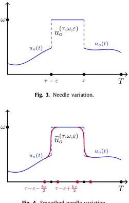
Now, for each given

τ ∈

(0

,

T

]

,

ω ∈

K

⊂

_RM_{and for each sufficiently small}

_{ε >}

_{0, let us denote by u}(τ,ω,ε)

o

: [

0

,

T

] →

K

the piecewise continuous map

u(τ,ω,ε)_o (t)

:=

⎧

⎪

⎪

⎨

⎪

⎪

⎩

uo(t) if t

∈

[

0

, τ − ε),

ω

if t

∈

[

τ − ε, τ),

uo(t) if t

∈

[

τ,

T

]

(6.2) and denote by

˜

u (τ,ω,ε)

o

: [

0

,

T

] →

K a smooth map, which appropriately approximates u(τ,ω,ε)o , i.e. it coincides with it at

all points with the only exception of two ‘‘very’’ small neighborhoods of the discontinuities at t

=

τ − ε

and

τ = τ

.8We call u(τ,ω,ε)o the needle variation at t

=

τ

of ceiling value

ω

and width

ε

. Any associated continuous approximation

˜

u

(τ,ω,ε)

o

will be called smoothed needle variation (seeFigs. 3and4).

Remark 6.1. A rigorous derivation of the classical PMP from our Principle of Minimal Labour should be built using the smoothed approximations

_˜

u(τ,ω,ε)o of the needle variations. However, with the purpose of being as much as possible direct

and clear, here we use the (discontinuous) needle variations u(τ,ω,ε)o . It is true that the fact that the u(τ,ω,ε)o are notC∞can

make some of our arguments sounding not completely right. Note however that everything is immediately fixed by just considering smoothed needle variations in place of the discontinuous ones.

Given a needle variation u_ε(t)

:=

u(τ,ω,ε)o (t) of uo(t), we denote by

U_ε

=

(u_ε(t)

,

(ao

,

bε))

the unique pair in

˜

K

′

, with first element given by u_ε(t) and second element given by the pair (ao

,

bε) of initial values,

chosen so that the corresponding curve

γ

(Uε) satisfies the condition(5.3)on the final value p(T ). We also consider the homotopy

γ

_ε(t

,

s)

=

γ

(Uε(s))(t), where U_ε(s)

=

(u(s,ε)(t)

,

(ao

,

b(s,ε))) is the unique curve in the set

˜

K

′

, in which – u(s,ε)(t) is defined by (seeFig. 5)

u(s,ε)(t)

:=

(1

−

s)uo(t)

+

suε(t)

.

(6.3)

– the initial values (ao

,

b(s,ε)) are chosen so that each curve

γ

ε(t

,

s)

=

γ

(Uε(s))(t), s

∈ [

0

,

1

]

, satisfies the condition(5.3) on p(T ).

Fig. 5.

Fig. 6.

Such homotopy

γ

_ε, connecting the curves

γ

(Uo) _and

γ

(Uε)_{, uniquely determines the associated 2-dimensional labour} W(Uo,Uε,γε)_.

Now, given

τ ∈

(0

,

T

]

and

ω ∈

K

⊂

_{R and setting uε}(t)

:=

u(τ,ω,ε)o (t), for a sufficiently small interval (0

, ¯ε

), we may

consider the function

W

:

(0

, ¯ε

)

−→

_R

,

W (

ε

)

:=

W(Uo,Uε,γε)

_.

We have that (Fig. 6):

(1) The function W is non-negative (by the Principle of Minimal Labour);

(2) The definition of W (

ε

) does not make any sense for

ε =

0; in fact, there is no possible smoothed variation

_˜

u(τ,ω,ε)o (t)

when

ε =

0; nonetheless W (

ε

) can be extended at

ε =

0 by setting W (0)

=

lim_ε→0W (

ε

)

=

0;

(3) The function W (

ε

) is differentiable at all points

ε >

0, but, a priori, it might not be differentiable at

ε =

0.

However, by (1), (2) and (3), it follows that if lim_ε→0dW_dε

⏐

⏐

_ε is proved to exist, then we have that W is differentiable also

at 0 with non-negative derivative at 0, i.e.

dW d

ε

⏐

⏐

⏐

⏐

ε=0

=

lim ε→0 dW d

ε

⏐

⏐

⏐

⏐

ε

≥

0

.

The limit lim_ε→0dW_dε

⏐

⏐

εdoes actually exist and it can be checked as follows. First of all, observe that for any

ε ∈

(0

, ¯ε

),

∂

∂

su (s,ε)_(t)

₌

_u ε(t)

−

uo(t)

=

⎧

⎪

⎪

⎨

⎪

⎪

⎩

0 if t

∈

[

0

, τ − ε),

ω −

uo(t) if t

∈

[

τ − ε, τ),

0 if t

∈

[

τ,

T

]

.

Thus, from(5.2), W(Uo,Uε,γε)

_{= −}

∫

s=1 s=0

(

∫

τ τ−ε

(

ω

ℓ

₋

_uℓ o(t)

)

∂

H

∂

uℓ

⏐

⏐

⏐

⏐

(t,q(s,ε)_(t),p(s,ε)_(t),u(s,ε)_(t)) dt

)

ds

and, for any fixed

ε

o

∈

(0

, ¯ε

) dW(Uo,Uε,γε) d

ε

⏐

⏐

⏐

⏐

εo

= −

∫

s=1 s=0

(

ω

ℓ

₋

_uℓ o(

τ − ε

o)

)

∂

H

∂

uℓ

⏐

⏐

⏐

⏐

(

t,q(s,εo )_(τ−εo),p(s,εo )_(τ−εo),u(s,εo )_(τ−εo)

)

ds

−

∫

s=1 s=0

(

∫

τ τ−εo

(

ω

ℓ

₋

_uℓ o(t)

)

·

∂

∂ε

[

∂

∂

uℓH

(

t

,

q(s,ε)(t)

,

p(s,ε)(t)

,

u(s,ε)(t)

)

]

ε=εo dt

)

ds

.

It is now sufficient to observe that the second summand on the right hand side of this expression goes to zero for

ε

o

→

0

(by the Lebesgue Theorem on quasi-continuity) and that lim_εo→0dW (Uo,U_ε,γ) dε

⏐

⏐

⏐

⏐

εo

exists and is equal to

d d

ε

W (Uo,Us,γ)

⏐

⏐

ε=0

= −

∫

s=1 s=0

(

ω

ℓ

₋

_uℓ o(

τ

)

)

∂

H

∂

uℓ

⏐

⏐

⏐

⏐

(t,q(τ),p(τ),(1−s)uo(τ)+sω) ds

= −

∫

s=1 s=0

∂

∂

sH(t

,

q(

τ

)

,

p(

τ

)

,

(1

−

s)uo(

τ

)

+

s

ω

)ds

= −

H(

τ,

q(

τ

)

,

p(

τ

)

, ω

)

+

H(

τ,

q(

τ

)

,

p(

τ

)

,

uo(

τ

))

.

(6.4)

Since we already observed that by the Principle of Minimal Labour, one necessarily has that _dd_εW(Uo,Uε,γε)

⏐

⏐

_ε=0

≥

0, from

(6.4)the Pontryagin Maximum Principle follows. □

7. Principles of Minimal Labour in case of non-smooth data

As it has been pointed out in Section2, so far we have just considered classical Mayer problems that are determined by ingredientsK,G,K

↦→

G, I satisfying all assumptions of smoothness and regularity that render the line of the arguments as much as possible straightforward. It is now time to indicate to which extent our discussion can be generalized to Mayer problems with lower regularity assumptions or with additional terminal constraints.

Consider a control problem in which the ingredientsK,G,K

→

G, I are of the following kind.

•

The setKconsists of pairs of the form U

=

(u(t)

,

(a

,

b)), in which u(t) is aC2function u

: [

0

,

T

] →

K taking values

into a subset K

⊂

_RM, which might be disconnected or with empty interior.

•

The classGconsists ofC2curves in

[

0

,

1

] ×

T∗Mof the form(2.1).

•

For each U

∈

Kthe correspondence U

∈

K

↦→

γ

(U)

∈

G maps U

=

(u(t)

,

(a

,

b)) into the unique solution to the

differential problem(2.2)for someC2-function F (t

,

qi

_,

_uℓ_{) which is defined on a set of the form}

_[

₀

_,

₁

_{] ×}

_M

_×

_U K for

some convex neighborhoodU_K

⊂

_RM of K .

•

The cost functional I has the form(2.6)with

α

as in(3.2)with C (t

,

q) of classC2_on

_[

₀

_,

₁

_{] ×}

_{Mand satisfying(3.3).} Let us also denote by

˜

Kthe subclass ofKdefined in (b) of Section3, so that the control problem, which is determined

byK

˜

, is precisely a classical Mayer problem on the curves

γ

(U)_(t)

₌

_(t

_,

_q(t)

_,

_{p(t)) with the initial value q(0)}

₌

_a

o.

The above regularity assumptions on the u(t), F (t

,

q

,

u) and C (t

,

q) lead to the following fact. Consider two curves uo(t)

and u(t) with values in K

⊂

_Rmand pick aC2-homotopy of curves u(t

,

s) such that:

(a) it varies between uo(

·

)

=

u(

·

,

0) and u(

·

)

=

u(

·

,

1);

(b) it takes values inUK (but not necessarily just in K ).

Then, let U(s), s

∈ [

0

,

1

]

, be a curve of pairs of the form U(s)

=

(u(

·

,

s)

,

(ao

,

b(s))), with b(s) of classC2, and set Uo

:=

U(0)

and U

:=

U(1). Notice that, by construction, the endpoints Uo, U of the curve U(s) are both in

˜

K, but for s

̸=

0

,

1 the pairs

U(s) are not necessarily in

˜

K.

These assumptions imply that:

(1) The surfaceS(Uo,U)

_{⊂ [}

₀

,

_T

_{] ×}

_T∗_{M, spanned by the (traces of the) solutions}

γ

(U(s)) _{to(2.2)with data U(s)}

₌

(u(t

,

s)

,

(ao

,

b(s))), is actually the image of aC2-embeddingS

ˆ

(Uo,U)

: [

0

,

T

] × [

0

,

1

] → [

0

,

T

] ×

T

∗

M; (2) All coefficients of the 1-form

α

are of classC1;

(3) The identity(4.6)holds also in this situation.

The claim (3) follows from the fact that the Stokes Theorem is still valid under the regularity properties (1) and (2) (see e.g. [12, Ch. 20, §6]).

Due to this, the same arguments considered in Section 4immediately yield to the following: an element Uo

∈

˜

Kis

between the curves

γ

(Uo)_and

γ

(U)_{, generated by homotopies u(t}

,

_{s) with values in the convex open setU}

K (but not necessarily

just in K ) with the above described regularity, the sum between the endpoint labourC(Uo,U,γ) _{and the 2-dimensional labour}

W(Uo,U,γ)_satisfies

C(Uo,U,γ)

₊

_W(Uo,U,γ)

_≥

₀

_.

_(7.1)

If we further restrictK

˜

to the proper subset

˜

K

′

that is determined by the terminal condition(5.3)and if we constrain the homotopies to be made of curves, determined by pairs U(s)

=

(u(t

,

s)

,

(ao

,

b(s))) that are all satisfying(5.3), then

(7.1)simplifies intoW(Uo,U,γ)

_≥

_{0. This gives a version of the Principle of Minimal Labour holding under the above described}

weaker regularity assumptions and in case of a set K

⊂

_RM_{, which may be disconnected or with empty interior.}

The fact that K is not required to be connected or with non-empty interior is not truly surprising. In fact, the hypotheses that allow to derive the Principle of Minimal Labour are basically just the openness and the convexity (or, more generally, the path connectedness) of the open set

[

0

,

1

] ×

M

×

UK, where the function F (t

,

qi

,

uℓ) is well defined and of classC2.

Starting now from this new version of the Principle of Minimal Labour, the previous proof of the Pontryagin Maximum Principle is still working. In this way we get the PMP also in case of a (possibly disconnected) set K and with the above mild regularity assumptions on F (t

,

q

,

u), C (t

,

q) and u(t).

A further weakening of the regularity assumptions can be very likely reached as follows. Instead of requiring that each curve u

: [

0

,

T

] →

K isC2, we may just impose that it is piecewiseC2-regular, i.e. that it is a possibly discontinuous function for which there is a finite number of points tj

∈ [

0

,

T

]

with the property that each restriction u

|

(ti,ti+1) is C

2 andC2-extendible to the closed interval

[

titi+1

]

. In this case, even if the surfaces S(Uo,U) that are spanned by the usual homotopies of curves

γ

(U(s)) _{cannot be expected to be C}2_{, it is reasonable to predict that they are nonetheless finite} unions ofC2-surfaces, provided of course that the function F (t

,

qi

,

uℓ), which appears in(2.2), is of classC2. Using such a decomposition inC2-pieces, one can still apply the Stokes Theorem to each C2 piece of the surface and obtain the inequality(7.1)also in these cases. Summing up, we expect that the Principle of Minimal Labour can be obtained and yield to a proof of the PMP also under such weaker assumptions.

Variants of the Principle of Minimal Labour with weaker regularity are out of reach if we limit ourselves to the above quoted version of the Stokes Theorem.

On the other hand, it is very well known that the PMP has already been proved in more general settings, as for instance those in which the u(t) are merely bounded and measurable and F (t

,

qi

_,

_uℓ_{) is just continuous (see e.g. [6, Ch. 6] for precise}

statements). We believe that these more general versions can be deduced from the above ‘‘piecewise smooth’’ PMP using approximations. A full clarification of this expectation would be useful and we hope to address it in a future work. It would pave the way to a systematic two-step use of the Principle of Minimal Labour: first, begin with piecewise smooth data and infer from the Principle of Minimal Labour not only the PMP but also statements of other necessary conditions on the optimal solutions (see, for instance, those hinted in Section8.2); second, find a way to prove the new statements also in case of weaker regularity using approximations.

8. Further consequences of the principle of Minimal Labour

8.1. The labour functional

The Principle of Minimal Labour admits the following equivalent presentation. Let Uo

=

(u(t)

,

(ao

,

b)) be a pair in the

restricted class

˜

K

′

. As usual, for any other U

∈

K

˜

′

let us consider a homotopy of curves

γ

(t

,

s)

=

γ

(U(s))_{(t), determined by} a curve U(s)

∈

˜

Kconnecting Uowith U. Note that, for each choice of a point Uλ,

λ ∈ [

0

,

1

]

, of the curve U(

·

)

∈

K

˜

′ , it is possible to rescale the parameter and obtain in this was a new homotopy, having the curves corresponding to Uoand Uλ

as endpoints:

γ

λ

: [

0

,

T

] × [

0

,

1

] → [

0

,

T

] ×

T∗

RN

,

γ

λ(t

,

s)

:=

γ

(t

, λ

s)

.

(8.1)

In this way, each pair (U

, γ

), formed by a fixed U

∈

˜

K

′

and a homotopy

γ

(t

,

s)

=

γ

(U(s))_{(t), connecting}

_γ

(Uo) _and

_γ

(U)_, automatically determines an entire new one-parameter family of pairs (U_λ

, γ

_λ), formed by U_λ

=

U(

λ

) and the homotopy, which is defined in(8.1)and connects the curve

γ

(Uo) _{with the curve}

_γ

_{(Uλ). It goes without saying that, conversely, a} one-parameter family of pairs (U_λ

, γ

_λ),

λ ∈ [

0

,

1

]

, as above, where the homotopies have the form

γ

λ(t

,

s)

=

γ

₁(t

, λ

s) for each

λ ∈ [

0

,

1

]

,

(8.2)

is uniquely determined by final pair (U

, γ

)

:=

(U_λ=1

, γ

λ=1), corresponding to the value

λ =

1.

This simple observation suggests that, for each pair (U

, γ

) as above, one can consider the function (seeFig. 7) W

: [

0

,

1

] →

R

,

W(

λ

)

:=

W(Uo,Uλ,γλ)

= −

∫ ∫

t∈[0,T],s∈[0,1] H_uℓ

⏐

⏐

(γ(λs)_{(t),u(t,λs))}

∂

uℓ(t

, λ

s)

∂

s

⏐

⏐

⏐

⏐

_(t, s) dt ds

= −

λ

∫ ∫

t∈[0,T],s∈[0,1] H_uℓ

⏐

⏐

(γ(λs)_{(t),u(t,λs))}

∂

uℓ(t

,

s′ )

∂

s′

⏐

⏐

⏐

⏐

_(t, s′=λs) dt ds

.

Fig. 7.

We call this function the labour function of the homotopy

γ

(t

,

s)

=

γ

(U(s))_{(t). Being W(0)}

=

0, we can formulate the Principle of Minimal Labour in the following equivalent form.

Principle of Non-Negative Labour Functionals. Necessary and sufficient condition for an element Uo

∈

˜

K

′

to be a p-optimal solution is that for each pair (U

, γ

) as above, the corresponding labour function W(

λ

) has a minimum at

λ =

0.

As immediate consequence of this statement is that Uo

=

(uo(t)

,

(ao

,

b)) is a p-optimal solution (thus an optimal one)

only if dW d

λ

⏐

⏐

⏐

⏐

λ=0

= −

∫ ∫

t∈[0,T]_,s∈[0,1] H_uℓ

⏐

⏐

_(γ(Uo)(t), uo(t))Y ℓ

⏐

⏐

_(γ(Uo)(t), uo(t))dt ds

≥

0

.

(8.3)

for any of the vector fields of the form Y

=

Yℓ ∂_∂

uℓ, which are defined at the points (

γ

(Uo)_(t)

_,

_u o(t)) as Y

:=

∂

u ℓ_(t

_,

_s′ )

∂

s′

⏐

⏐

⏐

⏐

(t,s′=0)

∂

∂

uℓ

⏐

⏐

_(γ(Uo)(t), uo(t)) (8.4)

for some homotopy

γ

(t

,

s)

=

γ

(U(s))(t) corresponding to a curve U(s)

∈

˜

K

′

originating from Uo.

In the special situations, in which the homotopies

γ

(t

,

s)

=

γ

(U(s))_{(t) of the above kind are so many that, by means of} (8.4), they generate all possible vector fields of the form Y

=

Yℓ ∂_∂

uℓ at the points of the curve (

γ

(Uo)_(t)

,

_u

o(t)) (and thus

also the opposite

−

Y

= −

Yℓ ∂_∂

uℓ), condition(8.3)holds if and only if condition

∂

H

∂

uℓ

⏐

⏐

⏐

⏐

(t,q(t),p(t),uo(t))

=

0 for each t

∈ [

0

,

1

]

(8.5) is satisfied.

We remark that condition (8.3) (and its consequent pointwise version (8.5)) can be also obtained as a direct consequence of the classical Pontryagin Maximum Principle. In fact, (8.3)is sometimes considered as an infinitesimal version of such principle. However, the above line of arguments, which are independent of the classical PMP, makes clear the fact that, on the contrary,(8.3)and the classical PMP are indeed two independent consequences of the same necessary and sufficient criterion, namely of the Principle of Minimal Labour.

Note also that (8.3)and the PMP are obtained by taking the first derivatives of two different functionals: the first comes from derivatives of the Labour Functionals W(

λ

), determined by the homotopies

γ

(t

,

s); the second comes from

the functionals W (

ε

), determined by one-parameter families of needle variations u_ε

=

u(τ,ω,ε)and, consequently, by the

one-parameter families of homotopies

γ

_ε

= {

γ

_ε(

·

,

s)

,

s

∈ [

0

,

1

]}

(distinguished one from the other by the independent variable

ε

) defined in(6.3).

8.2. A few lines for further developments

Suppose that a pair Uo

=

(uo

,

(ao

,

b))

∈

˜

K

′ is such that

∂

H

∂

ua

⏐

⏐

⏐

⏐

(t,q(t),p(t),uo(t))

=

0 for each t

∈ [

0

,

1

]

.

(8.6)

Hence it trivially satisfies the necessary condition(8.5). The same ideas that led to(8.5)now imply that Uois optimal only

if, for any homotopy

γ

(t

,

s) as above, the second derivative at

λ =

0 of the labor functional W is non-positive.

Following this pattern, a whole sequence of necessary conditions could be obtained just by looking at the derivatives of higher order of the functional W, namely of order three, four and so on.

It is noteworthy to point out that several important generalized high order conditions have been already determined in the literature (see e.g. [13,22]). From what we can see at the moment, such conditions seem to be strictly related with

the necessary conditions that one can obtain from labour functionals by considering higher order derivatives at

λ =

0. An investigation of such higher order derivatives should necessarily include a careful comparison with the higher order conditions existing in the literature.

Another area of studies is suggested by the analogies and differences between the proofs of the classical PMP and the first order condition(8.3)or(8.5). Roughly speaking, they are both obtained by taking first derivatives of two functionals, of very different construction one from the other. Thus it might be worth to make a comparative study also of the (generalized) higher order derivatives of such two involved functionals.

Before concluding, we would like to point out that an analogue of the Principle of Minimal Labour exists for any control problem, in which the correspondence U

∈

K

↦−→

γ

(U)

_∈

_{Gis given by associating to an appropriate control parameter U} the solution

γ

(U)of Euler–Lagrange equations, determined by time-dependent Lagrangians of higher order and with cost functional depending on high order derivatives [11].

References

[1] M. Bardi, I. Capuzzo-Dolcetta, Optimal Control and Viscosity Solutions of Hamilton–Jacobi-Bellman Equations (with Appendices by M. Falcone and P. Soravia), Systems & Control: Foundations & Applications, Birkhäuser Boston, Inc., Boston, MA, 1997, xviii+570.

[2] Aldo Bressan, On control theory and its applications to certain problems for Lagrangian systems. On hyper-impulsive motions for these. II. Some purely mathematical considerations for hyper-impulsive motions. Applications to Lagrangian systems, Atti Accad. Naz. Lincei Rend. Cl. Sci. Fis. Mat. Nat. 8 (1) (1988) 107–118.

[3] Aldo Bressan, On the application of control theory to certain problems for Lagrangian systems, and hyper-impulsive motion for these. I. Some general mathematical considerations on controllizable parameters, Atti Accad. Naz. Lincei Rend. Cl. Sci. Fis. Mat. Nat. 8 (1) (1988) 91–105.

[4] Aldo Bressan, On control theory and its applications to certain problems for Lagrangian systems. On hyper-impulsive motions for these. III. Strengthening of the characterizations performed in Parts I and II, for Lagrangian systems. An invariance property, Atti Accad. Naz. Lincei Rend. Cl. Sci. Fis. Mat. Nat. 8 (3) (1990) 461–471.

[5] Alberto Bressan, Impulsive control of Lagrangian systems and locomotion in fluids, Discrete Contin. Dyn. Syst. 20 (1) (2008) 1–35.

[6] Alberto Bressan, B. Piccoli, Introduction to the Mathematical Theory of Control, American Institute of Mathematical Sciences (AIMS), Springfield, MO, 2007.

[7] Alberto Bressan, F. Rampazzo, On differential systems with vector valued impulsive controls, Boll. U.M.I 3-B (1988) 641–656.

[8] F. Cardin, Elementary Symplectic Topology and Mechanics, Lecture Notes of the Unione Matematica Italiana, vol. 16, Springer, Cham, 2015.

[9] F. Cardin, M. Favretti, On nonholonomic and vakonomic dynamics of mechanical systems with nonintegrable constraints, J. Geom. Phys. 18 (1996) 295–325.

[10] F. Cardin, M. Favretti, Hyper-impulsive motion on manifolds, Dyn. Contin. Discrete Impuls. Syst. 4 (1998) 1–21.

[11] F. Cardin, A. Spiro, Higher order equations with controls and generalizations of the Pontryagin Maximum Principle (in preparation). [12] S. Lang, Real Analysis, Addison-Wesley Publishing Company, Reading, MA, 1983.

[13] U. Ledzewicz, H. Schättler, A high-order generalized local maximum principle, SIAM J. Control Optim. 3 (2000) 823–854.

[14] C.-M. Marle, Sur la géométrie des systèmes mécaniques à liaisons actives, C. R. Acad. Sci. Paris Sér. I Math. 311 (1990) 839–845.

[15] C.-M. Marle, Géométrie des systèmes mécaniques à liaisons actives, in: Symplectic geometry and mathematical physics (Aix-En-Provence, 1990), Birkhäuser Boston, Boston, MA, 1991, pp. 260–287.

[16] M.R. Menzio, W.M. Tulczyjew, Infinitesimal symplectic relations and generalized Hamiltonian dynamics, Ann. Inst. Henri Poincaré XXVIII (1978) 349–367.

[17] L.S. Pontryagin, V.G. Boltyanskii, R.V. Gamkrelidze, E.F. Mishchenko, The Mathematical Theory of Optimal Processes (translated by D. E. Brown), The Macmillan Co, New York, 1964.

[18] F. Rampazzo, On Lagrangian systems with some coordinates as controls, Atti Accad. Naz. Lincei Rend. Cl. Sci. Fis. Mat. Nat. (8) 82 (1988) 685–695.

[19] F. Rampazzo, On the Riemannian structure of a Lagrangean system and the problem of adding time-dependent coordinates as controls, Eur. J. Mech. A Solids 10 (1991) 405–431.

[20] C. Sinestrari, Regularity along optimal trajectories of the value function of a Mayer problem, ESAIM Control Optim. Calc. Var. 10 (2004) 666–676.

[21] H.J. Sussmann, Geometry and Optimal Control, in: Mathematical Control Theory, Springer, New York, 1999, pp. 140–198.

[22] H.J. Sussmann, A Local Second- and Third-Order Maximum Principle, in Proceedings of the 2002 American Control Conference, held in Anchorage, AK, May (2002) 8-10, IEEE Cat. No.CH37301, 2002.

[23] H.J. Sussmann, J.C. Willems, The brachistochrone problem and modern control theory, in: Contemporary Trends in Nonlinear Geometric Control Theory and Its Applications (México City, 2000), World Sci. Publ., River Edge, NJ, 2002, pp. 113–166.

[24] H.J. Sussmann, J.C. Willems, Three Centuries of Curve Minimization: From the Brachistochrone to Modern Optimal Control Theory, 2003 (a book downloadable fromwww.math.rutgers.edu/~sussmann/papers/main-draft.ps.gz).