Code validation and model qualification for problems of mixing and thermal exchange in innovative reactors

del  cobeneficiario  

Code  validation  and  model  qualification  

for  problems  of  mixing  and  thermal  

exchange  in  innovative  reactors  

Nicola  Forgione,  Niccolò  Sanzo,  Francesco  Venturi  

CODE  VALIDATION  AND  MODEL  QUALIFICATION  FOR  PROBLEMS  OF  MIXING  AND  THERMAL  EXCHANGE  IN   INNOVATIVE  REACTORS  

Nicola  Forgione,  Niccolò  Sanzo,  Francesco  Venturi  (UNIPI)    

Settembre  2013    

Report  Ricerca  di  Sistema  Elettrico    

Accordo  di  Programma  Ministero  dello  Sviluppo  Economico  -­‐  ENEA   Piano  Annuale  di  Realizzazione  2012  

Area:  Produzione  di  energia  elettrica  e  protezione  dell'ambiente    

Progetto:  Sviluppo  competenze  scientifiche  nel  campo  della  sicurezza  nucleare  e  collaborazione  ai  programmi  internazionali  per  il   nucleare  di  IV  Generazione    

Obiettivo:  Sviluppo  competenze  scientifiche  nel  campo  della  sicurezza  nucleare   Responsabile  del  Progetto:  Felice  De  Rosa,  ENEA  

Il  presente  documento  descrive  le  attività  di  ricerca  svolte  all’interno  dell’Accordo  di  collaborazione  “Sviluppo  competenze   scientifiche  nel  campo  della  sicurezza  nucleare  e    collaborazione  ai  programmi  internazionali  per  il  nucleare  di  IV  generazione”   Responsabile  scientifico  ENEA:  Felice  De  Rosa.  

CIRTEN

Consorzio Interuniversitario per la Ricerca TEcnologica Nucleare

Lavoro svolto in esecuzione dell’Attività LP1-C2

AdP MSE-ENEA sulla Ricerca di Sistema Elettrico - Piano Annuale di Realizzazione 2012 Progetto B.3.1 “Sviluppo competenze scientifiche nel campo della sicurezza nucleare e collaborazione ai

programmi internazionali per il nucleare di IV generazione

UNIVERSITA’ DI PISA

Dipartimento di Ingegneria Meccanica, Nucleare e della Produzione

Code validation and model qualification

for problems of mixing and thermal exchange

in innovative reactors

(Validazione codici e qualifica modelli

per problematiche di miscelamento e scambio termico

in reattori innovativi)

2

Index

Summary ... 3

1. Introduction ... 4

2. Facility description ... 5

2.4 Data acquisition system ... 9

3. Experimental tests ... 10

3.1 Test Matrix ... 10

3.2 Test Procedure...10

3.3 Obtained results...10

4.

... 18

4.1 The computational domain ... 18

4.2 Numerical model ... 19

4.3 Monitored points ... 21

4.4 Matrix of simulations...22

4.5 Obtained results...24

4.6 Comparison of the obtained results...32

5. Conclusions ... 36

References ... 37

Nomenclature ... 38

3

Summary

The main objective of this work is to present the results obtained in the last campaign of experimental tests performed at the DIMNP (Department of Mechanical, Nuclear and Production) of the University of Pisa with a stainless steel mock-up, simulating the downcomer and lower plenum of a small scale PWR (Pressurized Water Reactor), in order to provide relevant data to study the mixing phenomena occurring during a DVI line break accident (SB-LOCA) and to validate commercial CFD codes.

These new tests are characterized by a cold water injection inside the downcomer from both the DVI lines.

The first part of this report is devoted to a brief recall of the description of experimental apparatus, hydraulic circuit and data acquisition system.

The second and most important part of the report is devoted to the description of the newly performed experimental tests.

The third part of the work is focused on numerical simulations, performed using the Fluent CFD code, and the main improvements introduced to the computational domain, in particular with regard to geometry and spatial discretization. The final part concerns a critical analysis of the comparison between experimental and computational data.

4

1. Introduction

The mixing phenomenon of the coolant in a nuclear reactor is an important mechanism of intrinsic safety against dilution of boron. In a PWR, boric acid is added to the coolant so as to compensate the excess reactivity of the fuel [1]. Non-uniformity in the mixing of boron is one of the most important safety topics of light water reactors; in fact, under certain operating or incidental conditions, formation of a fluid plume at low boron concentration is possible in the primary loop. When entering the core, without being mixed with water at nominal boron concentration, it may induce a risk of an accident due to insertion of positive reactivity [2].

The mixing phenomenon is not only important for nuclear safety, but also for structural integrity. In the case of LOCA, the cold water of the ECCS (Emergency Cooling System) is injected into the primary hot loop. When cold water comes into contact with the vessel walls, thermal stresses occur, which can compromise reactor pressure vessel integrity [3]. In addition, the mixing phenomenon is also important during the reactor’s normal operation, for example relating to coolant distribution temperature at the inlet of the core in the case of partial shutdown of the primary coolant pumps.

There are currently two methods for studying the boron mixing in the downcomer of a PWR: - experiments on a reactor scale model;

- numerical simulation: use of CFD techniques for the study of problems involving elements with three-dimensional geometries of possible large sizes.

However, in nuclear applications, numerical models require an initial experimental campaign in order to validate the results obtained by code simulations with results obtained experimentally. For this reason the most common procedure to study boron mixing in a downcomer and lower plenum of a PWR is a combined experimental and numerical approach [4].

This work was performed in the frame of the research programme on “New Nuclear Fission” funded by our Ministero dello Sviluppo Economico (Ministry of Economical Development) and co-ordinated by ENEA. In particular, it is oriented to perform a preliminary experimental campaign on a mock-up simulating the downcomer and lower plenum of a small scale pressurized reactor, categorized as Integrated Primary System nuclear Reactor (IPSR), in order to provide relevant data to study the mixing phenomena occurring during a DVI line break accident or during the operation of both lines without breakage.

5

2. Experimental facility description

The experimental facility, built at the DIMNP of Pisa University, consists of a stainless steel 1:5 scaled model of downcomer and lower plenum of the IRIS (International Reactor Innovative and Secure) reactor [5], designed with particular care to represent the geometrical configuration of the real plant (further details of the experimental facility are described in the previous report [6]).

In Figure 2.1 the test section is shown as drawing and as a photo performed on the lateral side.

Figure 2.1: Test section: drawing (left) and photos (right) [6]

2.2 Hydraulic circuit

The hydraulic circuit layout shown in Figure 2.2, consists of three different pipe lines:

- the primary line (red line), in which warm water, at a maximum temperature of 50°C, is sent to a manifold where the flow rate is equally divided among eight conical stainless steel pipes, simulating the eight downcomer mass flow inlets coming from the IRIS steam generators;

- the secondary line (blue line), which provides the required cold water flow to the two pipes simulating the DVIs located inside the IRIS downcomer;

- the tertiary line (green line), which controls the warm fluid temperature (water from the primary line).

The warm water, passing through the primary line, comes from a large water reservoir. The temperature of about ten cubic meters of water, contained in this large reservoir, was controlled by a heater system which includes three electrical heaters with a total maximum electrical power installed of 9 kW. Before starting the experimental test, the water contained in the large reservoir was heated to the desired temperature (less or equal to 50°C) circulating it only within the tertiary loop (acting on a three way valve). After the temperature set point was reached, the warm water was circulated through the primary line into the manifold and the heater system was bypassed. The high thermal capacity of the stored reservoir water allows tests to be performed in about one hour, without the activation of the HS, with a negligible reduction in water temperature inside the test section. When a test using cold water injection was foreseen the secondary line was also activated, injecting cold water from one or both the DVI pipes. In each pipe a regulator valve is present to precisely set the flow rate of the fluid.

6

Figure 2.2: Layout of the facility.

2.3 Instrumentation

The currently available measuring instrumentation, already described in the previous report, includes: - K-type TCs (thermocouples), to monitor the inlet and outlet test section fluid temperatures and fluid

temperatures at different locations inside the test section, to monitor temperature variations mainly in the lower plenum and at the “core inlet section”;

- an electromagnetic flow meter, placed on the pipe coming from the reservoir and shared with the primary and tertiary line;

- two regulator valves, model: "Caleffi 125141 L35 ΔkPa 22 - 220", used to set the mass flow rate in the two DVI pipes (shown in Figure 2.3).

All the measuring instruments have been calibrated by the manufacturer (as the electromagnetic flow meter) or directly in the laboratory (as for the TCs), to assess the uncertainty affecting every experimental data.

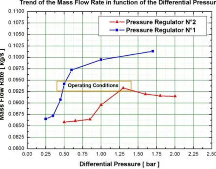
During the shake-down tests, problems were encountered on the data repeatability related to the evaluation of the mass flow rate injected by the two DVI lines. These data are obtained as an indirect evaluation through the measurement of differential pressure on a Venturi type nozzle present in each of the two DVI pipes. To characterize behavior of the two pressure regulators mounted on the DVI lines preliminary tests were planned and conducted in order to obtain the calibration curves, which shows the mass flow rate [kg/s] trend as a function of pressure differential to the regulators (see Figure 2.4). These tests consisted in flowing water through the regulator valve inserted in the DVI lines and collecting the water for a certain period of time. After weighing the water collected with precise scales it was possible to calculate the associated water mass flow rate.

7

Figure 2.3: Regulator valve, Model "Caleffi 125141 L35 ΔkPa 22 - 220".

The flow rate is controlled according to the value of ΔP which is measured through two piezometric inlets suitably positioned on the valve itself. On these inlets, it is possible to insert two pressure gauges, in such a way as to measure the ΔP on the Venturi's tube and prevent operation irregularities.

Figure 2.4: Calibration curves obtained for the two DVI flow rate regulators.

As can be seen the water flow rate and behavior of the two regulators are not perfectly constant, so, in order to inject a similar and constant water flow rate into the two DVI lines, two different values of differential pressure need to be set. In particular, the first regulator will be set at ΔP= 0.5 bar while the second regulator will be set at ΔP= 1.3 bar. With these values of differential pressure a mass flow rate of about 0.93 kg/s is generated for each DVI line.

8

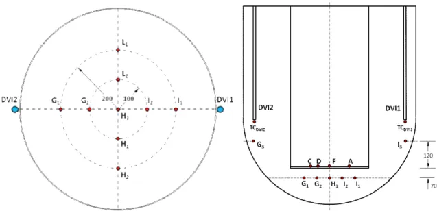
In Figures 2.5 and 2.6, respectively, the final disposal of the TCs that are placed just above the perforated plate and of those placed inside the semi-spherical shell in correspondence to the horizontal plane placed 0.07 m below the inlet section of the inner cylinder are shown.

Figure 2.5: Disposal of the TCs placed above the perforated plate.

Figure 2.6: TCs inside the semi-spherical part of the test section

9

2.4 Data acquisition system

The DAS (Data Acquisition System), utilized for the facility, already described in the previous report [6], converts and acquires the electrical signals coming from instrumentation present in the facility. Figure 2.7 shows a picture of the interactive control panel of the data acquisition system created with LabVIEW® software.

10

3. Experimental tests

3.1 Test matrix

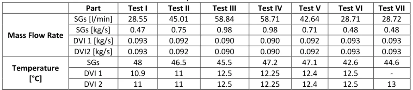
Seven different tests were performed with three different values of the nominal mass flow rate of warm water injected through the SGs (see Table 3.1). In particular, the first six tests are characterized by cold water injections in both lines with values of SGs's mass flow rate between 0.5 and 1 kg/s and DVIs's mass flow rate about 0.093 kg/s. The seventh test, however, is characterized by a single cold water injection by only the DVI2. For this new campaign of performed experimental tests it is tried to maintain a ΔT about 30°C in order to have a better reproducibility of the phenomenon of thermal mixing in the downcomer.

Table 3.1: Experimental test matrix.

Part Test I Test II Test III Test IV Test V Test VI Test VII

Mass Flow Rate

SGs [l/min] 28.55 45.01 58.84 58.71 42.64 28.71 28.72 SGs [kg/s] 0.47 0.75 0.98 0.98 0.71 0.48 0.48 DVI 1 [kg/s] 0.093 0.092 0.090 0.090 0.092 0.093 0.093 DVI2 [kg/s] 0.093 0.092 0.090 0.090 0.092 0.093 0.093 Temperature [°C] SGs 48 46.5 45.5 47.2 47.1 42.6 44.6 DVI 1 10.9 11 12.5 12.25 12.4 12.5 - DVI 2 11 11 12.5 12.25 12.4 12.5 13 3.2 Test procedure

The test procedure consists in an initial warm water injection from the eight conical entrances with appropriate mass flow rate, waiting until reaching, as much as possible, a uniform water temperature inside the test section. Then, a first phase of some seconds of cold water injection from the DVI follows, having the purpose of cooling the pipeline that connects the cold water reservoir with the test section. Due to the absence of thermal insulation on the external walls of the test section, thermal stratification phenomenon was observed inside the vessel, especially concentrated in the lower plenum. In fact, on the bottom side of the spherical region the temperature can result 2-3°C lower than the water temperature inside the downcomer. To avoid this phenomena during circulation of the warm water, just before the start of the test, a certain quantity of water was initially discharged from the bottom side of the spherical region, opening the discharging valve and checking temperature distribution inside the test section by looking at the data acquisition system. When an almost uniform water temperature was obtained inside all the test section, i.e. with a temperature variation less than 0.5°C, the cold water injection was started through the DVI2, keeping the DVI1 closed. In this first experimental campaign the duration of each test was set in the order of 10-12 minutes.

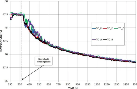
3.3 Obtained results

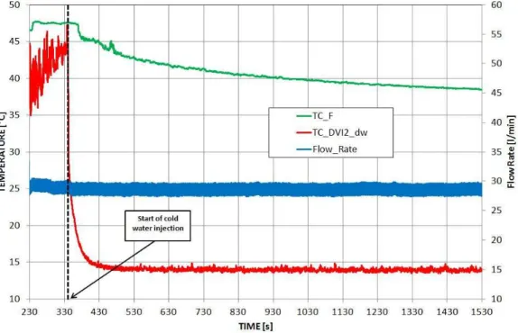
In Figure 3.1 a,b and c the time trend of both temperatures of the TCs placed at the exit section of the DVI lines inside the vessel (TC-DVI1_dw and TC_DVI2_dw) and positioned at the center of the perforated plate (TC-F) is reported. In the same figure the mass flow rate of warm water entering the eight conical pipes is also reported. As can be seen from Figure 3.1 a,b and c injection of cold water from the two DVI lines gives, respectively, a reduction of about of 7°C (Test I), 5°C (Test II) and 3°C (Test IV), on the center of the perforated plate. This reduction required about 100 s of transient from the beginning of the cold water injection to reach the asymptotic value and temperature reduction starting with a delay of about 20 s in respect to what was observed for the TC-DVIs.

11

Figure 3.1-a: Temperature and mass flow rate time trends (Test I).

12

Figure 3.1-c: Temperature and mass flow rate time trends (Test IV).

The same temperature trend as the TC-F can be observed for all the TCs placed above the perforated plate (see Figure 3.2 a,b and c).

13

Figure 3.2-b: Temperature time trends from TCs placed above the perforated plate (Test II).

Figure 3.2-c: Temperature time trends from TCs placed above the perforated plate (Test IV). Looking with attention at the trends reported in Figure 3.2 a,b and c, it is possible to conclude that the reduction in temperature is equal and symmetrical in both directions x and y of the porous plate. This behaviour is confirmed by examination of the temperature measured from the TCs placed on the horizontal plane at 0.07 m below the “core inlet” (see Figure 3.3 a,b and c).

14

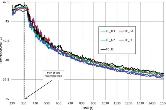
Figure 3.3-a: Temperature time trends from TCs located on the horizontal plane placed at 0.07 m below the inlet section of the inner cylinder (Test I).

Figure 3.3-b: Temperature time trends from TCs located on the horizontal plane placed at 0.07 m below the inlet section of the inner cylinder (Test II).

15

Figure 3.3-c: Temperature time trends from TCs located on the horizontal plane placed at 0.07 m below the inlet section of the inner cylinder (Test IV).

The temperature differences of the temperatures in the “core inlet section” are in this case in the order of 0.5°C maximum.

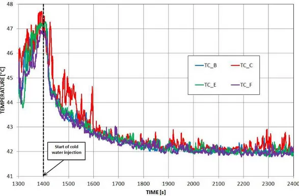
Test VII reproduces the incidental transient characterized by a single cold water injection

(in this case: only line DVI 2). Figure 3.4 a, b and c shows the trends of the flow rate, the temperature on the perforated plate and the temperature in the horizontal plane at 0.07 m below the “core inlet”.

16

Figure 3.4-b: Temperature time trends from TCs placed above the perforated plate (Test VII).

Figure 3.4-c: Temperature time trends from TCs located on the horizontal plane placed at 0.07 m below the inlet section of the inner cylinder (Test VII).

The maximum variation of temperature on the perforated plate is about 4 °C, the time necessary (about 650 s) to obtain such a variation is about double compared to that found in the same test characterized by cold water injection in both lines. The temperature distribution is not uniform on the horizontal plane placed at 0.07 m below the inlet section of the inner cylinder. In this case the TC-I1 shows a significantly lower value of temperature respect to the other TCs placed on the same plane. This means that the cold

17

water injected from the two DVI lines flows upward through the inner cylindrical shell preferentially on the opposite radial side respect to the injection position. As can be seen, the TC-I1, placed on the opposite radial side respect to the DVI2, shows a lower temperature value respect to the other TCs.

18

4. CFD simulation

The more detailed description of the computational domain and of the adopted numerical model was reported in previous reports [6-7]. Here a short description of the most important changes that have been imported into the computational domain is introduced.

4.1 The computational domain

The main changes imported to the computational domain, in order to obtain very close results to the experimental ones, are three and associated principally to the geometry of the system:

- the length of cold water injection tubes (DVI) was increased from 0.804 to 0.820 m;

- the internal diameter of cold water injection tubes (DVI) was increased from 0.015 to 0.0165 m;

- the distance between the internal wall of the cylindrical shell and the axis of the tube (DVI) was set at 90 mm.

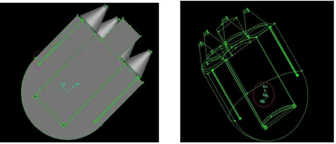
The total number of cells necessary for the discretization of the fluid volume has been suitably reduced to obtain a higher speed of calculation, passing from 4,700,000 (old configuration) to about 3,700,000 (new configuration). The new adopted 3D geometrical domain and the new unstructured mesh of the test section are shown in Figures 4.1 and 4.2, respectively. It must be noted that, because of symmetry, only half a test section was reproduced.

The origin of the coordinate reference system is positioned just on the symmetry plane at the vertical level in which the cylindrical part is connected to the spherical bottom part.

19

Figure 4.2: New spatial discretization: symmetry plane and DVI's inlet (left) and general view of the mesh of the system (right).

4.2 Numerical model

As already introduced in the previous report, since the Reynolds number assumes relatively high values in the downcomer, turbulent mixing is more important than molecular diffusion, [6]. Therefore, temperature and boron concentration profiles become similar once both the turbulent diffusivity coefficients assume values of the same order of magnitude.

Based on this assumption, in the facility the temperature field related to the mixing processes in the downcomer and lower plenum was investigated instead of boron concentration distribution.

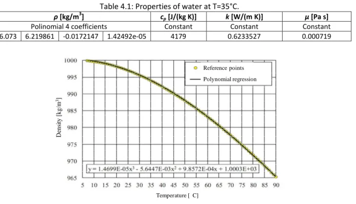
The working fluid considered in the simulations is water with the density set in the code as a function of temperature, in particular the behavior of the density function of the temperature has been described using a polynomial regression, while the values of viscosity, specific heat and conductivity were recruited at an average temperature of 35°C, (see Table 4.1).

Table 4.1: Properties of water at T=35°C.

ρ [kg/m3] cp [J/(kg K)] k [W/(m K)] μ [Pa s]

Polinomial 4 coefficients Constant Constant Constant 296.073 6.219861 -0.0172147 1.42492e-05 4179 0.6233527 0.000719 D en si ty [ k g /m 3] Temperature [ C] Reference points Polynomial regression

20

At the output of the eight cones the phenomenon of detachment of the fluid vein with a consequent non-uniformity of the speed on the output section of each cone occurs. The experimental solution adopted has been to place within each of these eight cones a flow divider with perforated plate at the bottom. In the numerical CFD code (FLUENT) the perforated plate is simulated as a porous region using the option Model Porous Media [4]. This model consists of adding a source term in equations standard flow that is composed of two parts: a term loss of viscous and inertial loss term.

where, Cij provides a correction for losses of load inertia in the porous medium. This constant can be

interpreted as a loss coefficient per unit length along the direction of flow. In the case of a perforated plate, it is possible to neglect the viscous loss term and consider only the term inertial loss, resulting in the following simplified form of the equation:

To calculate the coefficient Cij using the option "Using an Empirical Equation to Derive Porous Media

Inputs for Turbulent Flow Through a Perforated Plate ", which consist in using an empirical formula, in the case of a perforated plate, which allows to obtain such constant by the following equation:

where:

- t is the thickness of the perforated plate (porous medium);

- Ap is the total area of the plate (solid and holes);

- Af is the free area (total area of the holes);

- C2 is a constant whose value, for Re> 4000 and t/D> 1.6 (thickness to

diameter ratio plate), is 0.98. In this case a value of C2 equal to 500 was calculated.

To simulate the perforated plate present at the entrance of the inner cylinder the Porous Jump boundary condition (available in the calculation code [4]) was, instead, used. This condition is used to model thin membranes of known pressure drop. It is essentially a simplification of the 1D Porous Media Model described above. In this model the pressure loss is defined by the combination of a period of loss viscous and an inertial term according to the following formula:

where:

- is the viscosity of the fluid;

- is the permeability of the medium;

- C2 is the inertial loss coefficient (coefficient of pressure-jump);

- v is the normal component of the velocity of the fluid at the medium considered;

- is the thickness of the grid.

In this calculation the viscous term has been neglected by setting the value of the permeability very high. The inertial term is instead set at a value of K = C2 *Δm, where K can be calculated with some

empirical correlations for example, in this case, was used to Eckert & Pflugger [5]:

where, σ is the void ratio of the medium.

21

Due to obtain more information on the distribution of the fluid's speed and temperature inside the downcomer, in addition to the points that correspond to the real position of the thermocouples and those corresponding to the mass flow inlet/outlet surfaces, more points of interest are monitored. Table 4.2 shows the coordinates of all points monitored during evolution of the transient, while Figure 4.4 shows the layout of all points in the computational domain.

Table 4.2: Coordinates of all monitored points.

Points X [m] Y [m] Z [m] DVI 1 0 -0.538 -0.017 DVI 2 0 0.538 -0.017 A 0 -0.138 -0.367 B 0.138293 0 -0.367 C 0 0.138 -0.367 D 0 0.0915937 -0.367 F 0 0 -0.367 G1 0 0.2 -0.438 G2 0 0.1 -0.438 G3 0 0.538 -0.247 I1 0 -0.2 -0.438 I2 0 -0.1 -0.438 I3 0 -0.538 -0.247 H3 0 0 -0.438 L2 0.1 0 -0.438 L3 0.2 0 -0.438 N1 0 -0.538 -0.149 N2 0 0.538 -0.149 N3 0 -0.538 -0.037 N4 0 0.538 -0.037 N5 0 -0.2055 -0.367 N6 0 0.2055 -0.367 N7 0 -0.2400 -0.367 N8 0 0.2400 -0.367 N9 0.0691465 0 -0.367 N10 0.2074395 0 -0.367 F1 0 0 -0.333 F2 0 0 -0.149 A1 0 -0.138 -0.333 A2 0 -0.138 -0.149 C1 0 0.138 -0.333 C2 0 0.138 -0.149 N14 0 0 0.8

22

Figure 4.4: Layout of all monitored points.

4.4 Matrix of simulations

In this work four tests characterized by different values of mass flow rate were simulated with a CFD code (Fluent 13.0), temperature and porous jump coefficient (C2). In particular the first, second and third

tests are characterized by a increasing parallel cold water injection in both the DVI lines, while in the fourth test the cold water injection takes place only in a single DVI line (DVI 2).

The simulation test matrix, shown in Table 4.3.

Table 4.3: CFD simulation test matrix.

Part Test I Test II Test IV Test VII Mass flow rate [kg/s] SG 0.5 0.75 0.98 0.48 Single SG 0.0625 0.094 0.122 0.06 DVI1 0.093 0.092 0.090 - DVI2 0.093 0.092 0.090 0.093 Temperature [°C] SG 48 46.5 47.2 44.6 DVI1 UDF UDF UDF - DVI2 UDF UDF UDF UDF C2[1/m] 9884.2 9884.2 4000 2000

From the analysis of the previous experimental test campaign it has been seen that the cold water injection through the DVI lines does not occur like a step but needs a little time for the value of the temperature to reach the set point. In order to simulate this phenomenon with the calculation code was used the function: User-Defined Function (UDF) [8], by which it was possible to define the boundary condition (see an example in Table 3.4) to be provided as input to the DVI lines. UDF is a function, written in C programming language that when programmed can be dynamically loaded with the FLUENT solver to enhance the standard features of the code.

23 UDF_DVI 1 UDF_DVI 2 To t1 T0 T1 to t1 T0 T1 0 0.6 315.8 310.3 0 2.2 299.5 296.5 0.6 1.4 310.3 305.2 2.2 4 296.5 296 1.4 3.3 305.2 301.2 4 10.3 296 293.1 3.3 17.5 301.2 293.1 10.3 15.9 293.1 291.4 17.5 29.5 293.1 289.2 15.9 22.4 291.4 289.3 29.5 41.4 289.2 287.2 22.4 33 289.3 287.4 41.4 55.7 287.2 285.9 33 43 287.4 286.3 55.7 79.8 285.9 284.8 43 55.9 286.3 285.5 79.8 100.3 284.8 284.5 55.9 80.1 285.5 284.8 100.3 10*t0 284.5 284.2 80.1 99.8 284.8 284.5 99.8 10*t0 284.5 284.2 F_Profile=T0 + (T1 - T0) / (t1 - t0) * (f_time - t0)

where, t0,t1 and T0,T1 are, respectively the time/temperature steps of the transient.

Figure 4.5 shows the trend of the experimental cold water injection from the DVI lines (Test I) that have been described with the UDF.

Figure 4.5: Trend of experimental the cold water injection for Test I.

It is possible to notice a difference in temperature between the two lines at the beginning of the transient, this is due to the fact that the injected water from line 1 (DVI 1) must cover a greater distance and so it introduces a small delay.

24

For each test, steady state condition has been initially simulated without activation of the two DVI tubes. This preliminary simulation is required in order to define a correct initial condition from which a transient analysis is performed for the study of the flow and temperature fields following activation of the cold water injection from the two DVIs. Considering duration of the experimental tests and the computational time required for test simulation, the first 150 s of transient has been simulated. In fact, the main changes in temperature at the inlet core surface occurs during the first 100 s, after which there are slow changes in the average temperature (less than 0.5°C every 100 s).

The obtained results are shown for Test II (medium flow rate), the same observations and conclusions can be made for other tests (I and IV). The results are analyzed in terms of temperature and velocity fields. The used units are [°C] for the temperature and [m/s] for the velocity.

The simulation results are shown on two main planes: the symmetry plane and the ones normal to it. In Figure 4.6 a,b and c temperature distribution on the plane normal to the symmetry plane is shown for Test II at t = 30, 60 and 100 s of transient.

25

Figure 4.6-b: Temperature distribution on the symmetry plane for Test II (t = 60 s).

Figure 4.6-c: Temperature distribution on the symmetry plane for Test II (t = 100 s).

At the first 30 s of the transient a marked "U" shape distribution of the temperature at the entrance of the core can be noted (see Figure 4.6-a). This effect is due to the fact that fluid velocity at the inlet of inner cylinder does not have a negligible radial component and hence the fluid tends to move and pass next to the external side of the perforated plate. After 100 s of the transient this phenomenon is less marked and the temperature distribution, at the inner cylinder, is more uniform, (see Figure 4.6-c). Can be noticed a slight asymmetry of the temperature in correspondence of the porous plate, to be attributed to the normal evolution of the transient.

26

In Figure 4.7 a,b and c temperature distribution on the plane normal to the symmetry plane is shown for Test I at t = 30, 60 and 100 s of transient.

Figure 4.7-a: Temperature distribution on the plane normal to the symmetry plane for Test II (t = 30 s).

27

Figure 4.7-c: Temperature distribution on the plane normal to the symmetry plane for Test II (t = 100 s). As can be seen from Figure 4.7 a, b and c, there is a marked stratification between the two fluids, highlighted by the different colours of the hot fluid (orange) and the mixed fluid at the bottom hemispherical region. This phenomenon is more pronounced with the trend of the transient. The stratification is due to the different densities between the two water flows and to the higher velocity of the cold flow that exits the DVI tubes, combined with the geometry of the test section. At t = 100 s of the transient the temperature stratification has reached about half the length of the inner cylinder. In Figure 4.8 a and b distribution of streamline is shown for Test II at t = 30 and 100 s of transient.

Figure 4.8-a: Streamlines on symmetry plane for Test II (t = 30 s).

The analysis of Figures 4.8 a and b put in evidence the formation of vortices in the lower part of the downcomer, mainly due to the water jet from the two DVIs, that tend to drive the fluid radially towards

28

the entrance of the core region. This radial component of velocity is reduced inside the cylinder by its walls straightening the fluid after a central stagnating zone at the exit of the perforated plate.

Figure 4.8-b: Streamlines on symmetry plane for Test II (t = 100 s).

Figure 4.9: Velocity distribution on symmetry plane for Test II (t = 100 s).

The formation of vortices is clearly visible by analyzing the graph (see in Figure 4.9) which shows the velocity distribution on the symmetry plane, below and above the perforated plate. Immediately after passing the perforated plate, the velocity vectors are arranged in an orderly and linear motion to the exit.

In the next two Figures, 4.10 and 4.11, respectively, temperature distribution on the core inlet section and temperature distribution on a line positioned at a distance of -0.07 m from the previous is shown.

29

Figure 4.10: Temperature distribution on the core inlet section for Test II.

Figure 4.11: Temperature distribution on the line positioned at a distance z = -0.07 m for Test II. Analysis of the figures shows that temperature distribution, on both monitored surfaces, is symmetric with the central point (y = 0) at a lower temperature than the peripheral ones. After 100 s of the transient we can affirm that the temperature has almost reached a stationary state. Comparing calculated data with experimental, we can say that the temperature time trend is well reproduced by the CFD code.

30

For Test VII, characterized by a single cold water injection, temperature distribution and streamlines are shown for t > 100 s of the transient, (see Figure 4.12, 4.13 and 4.14). In fact, for t < 30 s of the transient temperature changes inside the downcomer are not sufficiently pronounced.

Figure 4.12: Temperature distribution on the symmetry plane for Test VII (t = 120 s).

The analysis of Figure 4.12 confirms what has been seen from the analysis of the experimental data: the point that is affected by a marked lowering of the temperature is located on the horizontal plane placed at 0.07 m below the inlet section of the inner cylinder positioned on the opposite side of the tube where the cold water exits.

31

Figure 4.13: Temperature distribution on the plane normal to the symmetry plane for Test VII (t = 120 s). From Figure 4.13 the phenomenon of thermal stratification of the fluid inside the downcomer can be noticed, unlike the previous case, this phenomenon affects a lower inner surface and temperature distribution is more regular. Furthermore it can be noted that in the upper part of the domain there is a marked accumulation zone of high temperature water, probably this area is not affected, in the first seconds, by heat exchange with the cold outlet water from the lines.

32

Analyzing the distribution of velocity on the the symmetry plane it is possible to note the formation of a single vortex at the inlet section of the inner cylinder, which, after having crossed the porous plate, tends to subside.

4.6 Comparison of the obtained results

Figure 4.15 a and b shows (for the Test II), in the first case, a comparison between the experimentally measured temperature and that obtained with CFD code in the central point of the perforated plate (F), while, in the second case, a comparison between the experimentally measured temperature and that obtained with CFD code in another point of the perforated plate (A).

33

Figure 4.15-b: Comparison between TC_A (exp.) and TC_A (CFD code), Test II.

Analyzing Figure 4.15 we can affirm that, in the first 60 s of transient, the temperature trend calculated with the CFD code follows the experimental one very well.

These results were obtained using a value of the porous jump coefficient (C2) equal to 9882.4 m -1

. Similar results were also obtained in Test I (low mass flow rate) and Test VII (single cold water injection), as shown in Figure 4.16 a and b and 4.17 a and b.

34

Figure 4.16-b: Comparison between TC_C (exp.) and TC_C (CFD code), Test I.

35

Figure 4.17-b: Comparison between TC_C (exp.) and TC_C (CFD code), Test VII.

As you can see from Figure 4.17 a and b, for the Test VII, the trend of TC_F and TC_C experimental temperature is very similar to that calculated by the CFD code in the first 90 s of transient. Subsequently we note a greater lowering of the calculated temperature compared to experimental trend, the difference is about one degree. Probably the non-uniformity between the two trends can be attributed to a too low value of the porous jump coefficient C2, which in this case was equal to 2000 m

-1

36

5. Conclusions

The aim of this work is to present the experimental and numerical analysis of thermal mixing in a test section that reproduces the downcomer and the lower plenum of an integrated PWR reactor (IPSR) with a scaling factor of 1/5.

The CFD analysis, performed using the commercial code Fluent has given more precise information about the phenomena that take place inside the downcomer of the reactor when there is an injection of cold water, this has been possible principally thanks to:

- refinement of the geometry of the computational domain to the real;

- increased of Δt (> 30 °C) between the warm water injected by the SG's and the cold water injected by the two DVI lines;

- refinement of the value to be adopted for the porous jump coefficient C2, to better estimate the

loss concentrated on the porous plate at the entrance of the cylinder.

These conducted simulations showed the influence on velocity of the vortices generated in the lower region in the proximity of the core entrance; this effect is to radially deflect the flow increasing the radial component of the velocity flow field in these regions. Those vortices are mainly due to the cold water injection from the DVI lines. Such velocity distribution caused the "U" shape observed for temperature distribution in the same region. Another conclusion deriving from experimental and calculated data concerns the presence of the inevitable thermal stratification between the two fluids at different temperatures, particularly favored by the geometry of the same downcomer.

From the comparison between experimental and calculated data, it can be affirmed that the code is a valuable tool that can reasonably reproduce the phenomena that occur during a thermal mixing transient in the downcomer region of an integrated PWR reactor, when the two DVI lines inject cold and borated water inside the vessel, even if some differences are present and must be investigated further.

37

References

[1] S. Kliem, U. Rohde, F.-P. Weiß, “Core response of a PWR to a slug of under-borated water”, Nuclear Engineering and Design, Vol. 230, pp. 121–132, 2004.

[2] V. Teschendorff, K. Umminger, FP Weiss, “Analytical and experimental research into boron dilution events”, Eurosafe Forum 2001, Seminar 2, Paris 2001.

[3] W. E. Burchill, “Physical Phenomena of a Small-Break Loss-of-Coolant Accident in a PWR”, Nuclear Safety, Vol. 23, No. 5, 1982.

[4] P. Gango, “Numerical boron mixing studies for Loviisa nuclear power plant”, Nuclear Engineering and Design, Vol. 177, pp. 239–254, 1997.

[5] M. D. Carelli, “IRIS: International Reactor Innovative and Secure”, Final Technical Progress Report STD-ES-03-40, November 2003.

[6] I. Angelo, V. Baduanza, N. Forgione, D. Martelli, "Characterization and validation of thermal and boron mixing phenomena in the downcomer and lower plenum of an integrated primary system nuclear reactor", Cerse-Unipi RL 1522/2011, Dipartimento di Ingegneria Meccanica, Nucleare e della Produzione, Università di Pisa, August 2012.

[7] N. Forgione, V. Baudanza, I. Angelo, D. Martelli, “Downcomer and lower plenum experimental facility”, Report RdS/2011/109, Report Ricerca di Sistema Elettrico, Accordo di Programma Ministero dello Sviluppo Economico – ENEA, settembre 2011.

38

Nomenclature

Abbreviations, acronyms and symbols

CFD Computational Fluid Dynamics

DAQ Data AcQuisition

DAS Data Acquisition System

DIMNP Dipartimento di Ingegneria Meccanica Nucleare e della Produzione DVI Direct Vessel Injection

ECCS Emergency Core Cooling System

HS Heater System

IRIS International Reactor Innovative and Secure LOCA Loss Of Coolant Accident

PWR Pressurized Water Reactor

SBLOCA Small Break Loss Of Coolant Accident

SCXI Signal Conditioning eXtensions for Instrumentation

TC Thermocouple K Inertial term σ Void ratio Re Number of Reynolds ρ Density μ Viscosity cp Specific heat k Conductivity

Ap Total area of the perforated plate

Af Free area of perforated plate

39

Breve CV del gruppo di lavoro

Nicola Forgione

Ricercatore in Impianti Nucleari presso il Dipartimento di Ingegneria Meccanica, Nucleare e della produzione (DIMNP) dell’Università di Pisa dal 20 dicembre 2007. Laureato in Ingegneria Nucleare nel 1996 presso l’Università di Pisa ed in possesso del titolo di Dottore di Ricerca in Sicurezza degli Impianti Nucleari conseguito all’Università di Pisa nel 2000. La sua attività di ricerca è incentrata principalmente sulla termofluidodinamica degli impianti nucleari innovativi, con particolare riguardo ai reattori nucleari di quarta generazione. Autore di oltre 20 articoli su rivista internazionale e di numerosi articoli a conferenze internazionali.

Nicolò Sanzo

Ha conseguito la laurea in Ingegneria Nucleare presso l'Università di Pisa nel 2013. A partire dallo stesso anno ha iniziato a collaborare con il DIMNP per analisi di fluidodinamica computazionale nell’ambito dell’ingegneria nucleare, in particolare utilizzato il codice CFD Fluent per l'analisi del miscelamento termico all'interno del downcomer di un reattore PWR integrato.