FONDO SOCIALE EUROPEO PROGRAMMA OPERATIVO NAZIONALE 2000/2006 “Ricerca Scientifica, Sviluppo Tecnologico, Alta Formazione”
Regioni dell’Obiettivo 1 – Misura III.4 - “Formazione superiore ed universitaria”
DOTTORATO DI RICERCA IN INGEGNERIA CIVILE PER L’AMBIENTE ED IL TERRITORIO
Università degli Studi di Salerno
VIII Ciclo Nuova Serie (2006-2009)
TESI DI DOTTORATO
WAVE ACTION ON SHALLOW WATER
AND APPLICATIONS TO COASTAL HAZARD
MARINA MONACO
Coordinatore del Dottorato Relatore
PROF. ING.RODOLFO M.A.NAPOLI PROF. ING.EUGENIO
PUGLIESE CARRATELLI
Correlatore
PROF. ING.ENRICO FOTI
WAVE ACTION ON SHALLOW WATER AND APPLICATIONS TO COASTAL HAZARD
__________________________________________________________________ Copyright © 2010 Università degli Studi di Salerno – via Ponte don Melillo, 1 – 84084 Fisciano (SA), Italy – web: www.unisa.it
Proprietà letteraria, tutti i diritti riservati. La struttura ed il contenuto del presente volume non possono essere riprodotti, neppure parzialmente, salvo espressa autorizzazione. Non ne è altresì consentita la memorizzazione su qualsiasi supporto (magnetico, magnetico-ottico, ottico, cartaceo, etc.).
Benché l’autore abbia curato con la massima attenzione la preparazione del presente volume, Egli declina ogni responsabilità per possibili errori ed omissioni, nonché per eventuali danni dall’uso delle informazione ivi contenute.
CONTENTS ... i
List of Symbols ... v
List of Abbreviations ... vii
List of Figures ... ix
List of Tables ... xiii
SOMMARIO ... xv
ABSTRACT ... xix
RESUME’ ... xxiii
RESUMEN ... xxvii
ACKNOWLEDGEMENTS ... xxxi
ABOUT THE AUTHOR ... xxxiii
1 INTRODUCTION ... 1
1.1 Context and aim of study ... 1
1.2 Outline of the thesis ... 2
2 MODELING FLUID FLOW ... 5
2.1 Numerical methods ... 5 2.2 Turbulence ... 7 2.3 RANS Equations ... 10 2.4 Turbulence models ... 12 2.4.1 K-ε model ... 13 2.4.2 RNG model ... 15 2.4.3 Wall function ... 15
2.5 Free surface displacement ... 17
2.5.1 Volume-of-Fluid (VOF) Method ... 18
2.7 Numerical implementation ... 21
2.7.1 Grid based systems ... 21
2.7.2 Stability condition ... 23
2.7.3 Numerical Viscosities ... 23
3 NUMERICAL METHODOLOGY of RANS/VOF MODELS .. 25
3.1 General Description of RANS/VOF models ... 25
3.2 Procedure of Simulation ... 27
3.3 Wave generation ... 28
3.3.1 Generation of waves using wave description theory ... 29
3.3.2 Generation of waves using a wave maker ... 31
4 SIMULATION OF REGULAR WAVES ON BEACH ... 33
4.1 Validation of the numerical model ... 33
4.2 Numerical setup ... 35
4.3 VOF and TrueVOF methods ... 37
4.4 Comparison between wave makers ... 41
4.5 Convergence analysis on computational discretization ... 43
4.5.1 Spatial discretization ... 43
4.5.2 Temporal discretization ... 50
4.6 Convergence analysis on turbulence models ... 51
4.6.1 Characteristic length scale ... 53
4.6.2 Turbulence Models ... 56
5 WAVE PROPAGATION ANALYSIS ... 59
5.1 Spilling on long sloping beach ... 59
5.2 Stokes drift ... 65
5.3 Reflection and Seiching ... 66
5.4 Breaking: types and criteria ... 69
iii
6 THE SCALE EFFECT ... 81
6.1 Hydraulic Similitude Theory ... 84
6.2 Limitations of Physical Modeling: the Scale Effects ... 85
6.3 The importance of scale effects on experimental results ... 86
6.4 Analysis on the scale effect ... 88
7 ENERGY AND MOMENTUM FLUX ... 99
7.1 General formulae for progressive waves ... 99
7.2 Wave energy for small amplitude theory ... 101
7.3 Numerical applications to non-breaking, breaking and reformed wave ... 104
7.4 Wave actions on a schematic structure ... 109
8 WAVE ACTION ON VERTICAL STRUCTURES ... 118
8.1 Hydraulic Pressures on Structures ... 118
8.2 Impact of Waves on Vertical Structures ... 123
9 CONCLUDING REMARKS ... 126
REFERENCES ... 130
v
LIST OF SYMBOLS
A wave amplitude
C propagation speed
Cg group velocities
d still water depth
E mean wave energy density per unit horizontal area e(t) energy density
F volume of fluid function
f general function
Fe energy flux
Fh horizontal force per unit extension of wall
Fqdm momentum flux
g acceleration of gravity
h local water depth
H wave height
H0 deep water wave height
Hs significant wave height K turbulent kinetic energy
k wave number
L wave length
L0 deep water wave length
m slope p pressure Q volume flow rate R run-up Sij radiation stress tensor t time in the physical domain
T wave period
u horizontal particle velocity along x axis
u' turbulence velocity
V horizontal particle velocity along y axis Vc volume of the cell
Vw volume of water inside a cell
w vertical particle velocity
x horizontal coordinate in the cross-shore direction y horizontal coordinate in the long-shore direction
z vertical coordinate
γb breaking parameter
Δx, Δy, Δz grid size
k Turbulent Kinetic Energy
ε Turbulent Kinetic Energy Dissipation Rate η surface elevation with respect to the mean level η* Kolmogorov length scale
θ slope angle
λ geometrical scale
μ dynamic viscosity
ν kinematic viscosity
νt turbulent kinematic viscosity
ξ surf similarity parameter ξ(t) wave-maker displacement
ρ water density
φ phase shift angle
Φ velocity potential
vii
LIST OF ABBREVIATIONS
CFD Computational Fluid Dynamics CFL Courant-Friedrichs-Levy DNS Direct Numerical Simulation
FAVOR Fractional Area/Volume Obstacle Representation
Fr Froude Number
LES Large Eddy Simulation
Ma Mach Number
MAC Marker And Cell
NS Navier Stokes
RANS Reynolds-Averaged Navier Stokes
Re Reynolds Number
RNG Renormalization-Group SPH Smoothed Particle Hydrodynamics
srfht Surface height
SWL Still water level
TKE Turbulent Kinetic Energy VOF Volume-Of-Fluid VPN Virtual Private Networking
ix
LIST OF FIGURES
Figure 2.1 : Energy cascade ... 9
Figure 2.2 : Approaches for the computation of turbulent flow ... 10
Figure 2.3 : Decomposition of a statistically stationary signal ... 11
Figure 2.4 : Decomposition of a not statistically stationary signal ... 11
Figure 2.5 : Wall bounded flow ... 16
Figure 2.6: Logarithmic velocity profile in a turbulent boundary layer ... 17
Figure 2.7: Free surface elevation as function of time ... 18
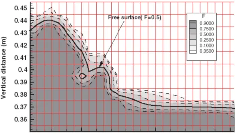
Figure 2.8: Typical values of the VOF function near free surface ... 19
Figure 2.9: Mesh arrangement and labeling convention ... 22
Figure 3.1: Location of variables in a mesh cell ... 26
Figure 3.2: Different types of wave generators ... 28
Figure 3.3: Schematic diagram showing a linear wave coming from a flat bottom reservoir on the right into the computational domain through the mesh boundary. ... 29
Figure 3.4: Wave generated by piston motion ... 32
Figure 4.1: General numerical set-up ... 33
Figure 4.2: Experimental images from Ting & Kirby (1996): a) spilling; b) plunging ... 34
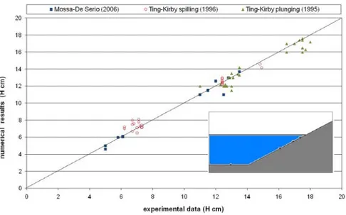
Figure 4.3: Correlation between numerical and experimental wave heights at different probes ... 34
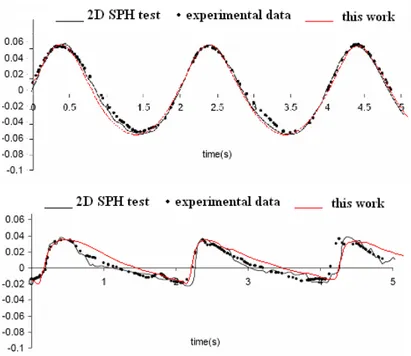
Figure 4.4: Comparison between instantaneous water height η, from experimental data, FLOW-3D numerical results and 2D SPH (from De Padova 2008a) ... 35
Figure 4.5: Numerical set up ... 37
Figure 4.6: Three steps of the Lagrangian interface tracking method: a) piecewise linear interface reconstruction with the normal n; b) moving the control volume; c) overlaying the advected volume onto the grid. ... 38
Figure 4.7: Volume of Fluid as function of time ... 39
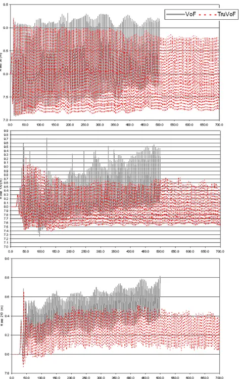
Figure 4.8: Surface Height as function of time in the probes P1, P2 and P3 ... 40
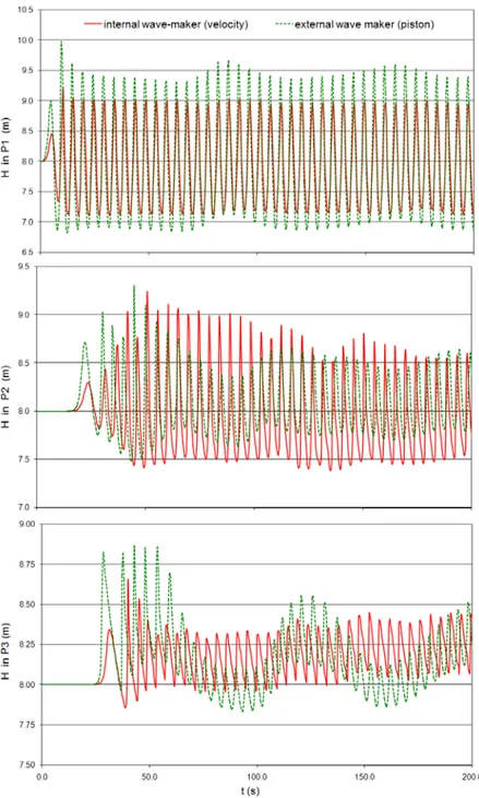
Figure 4.9: Wave height in the tree probes by internal and external wave makers ... 42
Figure 4.11: Comparison between wave height at different grid size: coarser grid; medium grid; finer grid ... 45
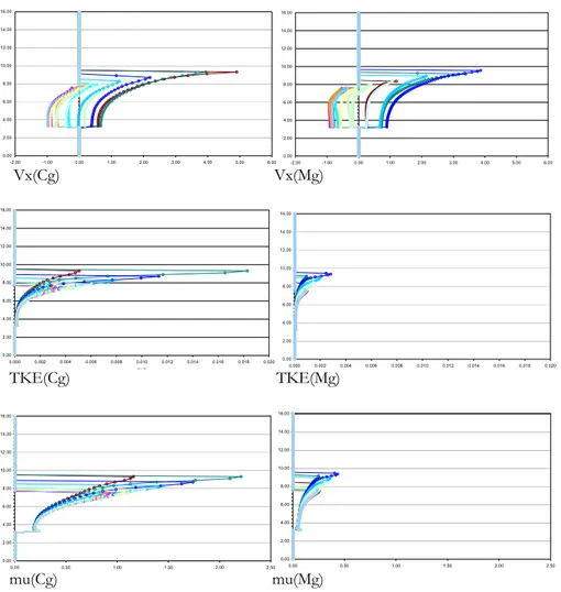
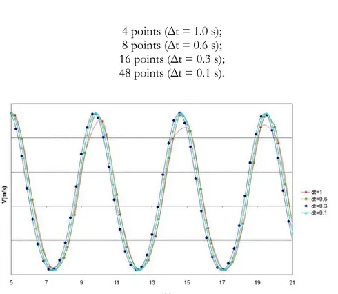
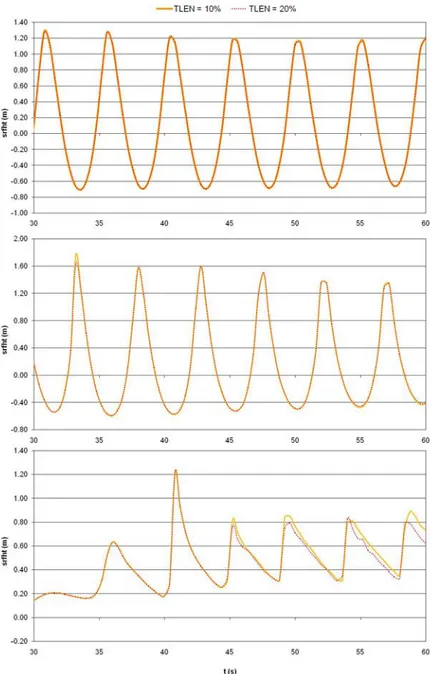
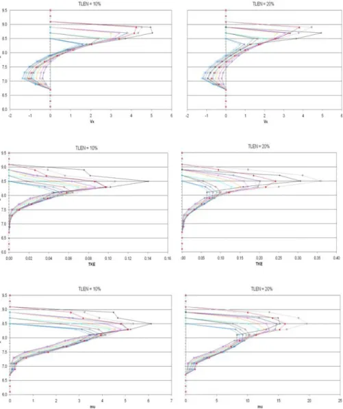
Figure 4.12: Vertical profile of horizontal velocity (Vx), turbulent kinetic energy (TKE) and dynamic viscosity (Mu) at different grid sizes (coarse grid on the left and medium grid on the right) in the probe P1 ... 47 Figure 4.13: Vertical profile of horizontal velocity (Vx), turbulent kinetic energy (TKE) and dynamic viscosity (Mu) at different grid sizes (coarse grid on the left and medium grid on the right) in the probe P2 ... 48 Figure 4.14: Vertical profile of horizontal velocity (Vx), turbulent kinetic energy (TKE) and dynamic viscosity (Mu) at different grid sizes (coarse grid on the left and medium grid on the right) in the probe P3 ... 49 Figure 4.15: Input velocity with different temporal increment ... 51 Figure 4.16: Influence of different TLEN on wave height in probes P1, P2, P3 ... 54 Figure 4.17: Influence of different TLEN on horizontal velocity,
turbulent kinetic energy and dynamic viscosity vertical profiles in probe P3 ... 55 Figure 4.18: Influence of turbulence models on the wave height in P1, P2 and P3 ... 56 Figure 4.19: Influence of turbulence models on the horizontal velocity in P3 (broken wave) ... 57 Figure 5.1: Numerical set-up of long sloping beach ... 59
Figure 5.2: Comparison between wave height in different probes: variable grid size; constant grid size ... 61
Figure 5.3: Comparison between wave height in different probes with a constant grid size: 20cm; 15cm. ... 62
Figure 5.4: Wave elevation in the constant depth zone as function of place: a) short sloping beach; b) long sloping beach. ... 64 Figure 5.5: Left boundary volume flow rate ... 65 Figure 5.6: Incident, Reflected and Total wave ... 67 Figure 5.7: Wave elevation as function of time in the probe 170 for the short sloping beach ... 68 Figure 5.8: Surface height at t=96.60s ... 70 Figure 5.9: Surface height for different breaking wave: a) spilling;
xi Figure 5.10: Surface height for a natural beach. a) field data; b) numerical
results ... 73
Figure 5.11: Verification of the classical breaking criterion ... 73
Figure 5.12: Horizontal velocity at breaking point ... 74
Figure 5.13: Turbulence generation and localization at different time: 1-2-3-4) spilling; 5-6-7-8) plunging (photos by Ting and Kirby laboratory experiments) ... 75
Figure 5.14: Turbulent Kinetic Energy amount and localization at different time and for different breaking types: a) spilling; b) plunging ... 76
Figure 5.15: Turbulent Kinetic Energy amount and localization at different time and for different breaking types: a) spilling; b) plunging ... 77
Figure 5.16: Definition of wave runup ... 78
Figure 5.17: Numerical results: (1) free surface elevation above bottom; (2) free surface elevation above still water level ... 80
Figure 6.1: Processes and relevant similitude laws for wave motions .... 87
Figure 6.2: Scale effect on the wave height at different probes P1, P2 and P3: / full scale; / scale 1:40; /scale 1:80 ... 90
Figure 6.3: Scale effect on the horizontal velocity at different probes P1, P2 and P3 ... 91
Figure 6.4: Scale effect on the turbulent kinetic energy at different probes ... 93
Figure 6.5: Scale effect on the eddy viscosity at probe P1 ... 94
Figure 6.6: Scale effect on the eddy viscosity at probe P2 ... 95
Figure 6.7: Scale effect on the eddy viscosity at probe P3 ... 96
Figure 6.8: Scale effect on the undertow profiles at different probes .... 97
Figure 7.1: Flux for a sinusoidal wave ... 103
Figure 7.2: Numerical set-up ... 104
Figure 7.3: Time history of momentum flux in probe P1 (linear wave), P2 (breaking wave) and P3 (reformed wave) ... 106
Figure 7.4: Wave height and momentum flux time histories in probe P1 for different H ... 107
Figure 7.5: Wave height and momentum flux time histories in probe P3 for different H ... 108
Figure 7.6: Numerical set-up with schematic structure, waters height and momentum fluxes at the wall as function of time: scheme A ... 110
Figure 7.7: Numerical set-up with schematic structure, waters height and momentum fluxes at the wall as function of time: scheme B ... 111 Figure 7.8: Surface elevations and momentum fluxes at the wall for
different incident waves: a) T=4.8s ... 112 Figure 7.9: Surface elevations and momentum fluxes at the wall for
different incident waves: b) T=10s ... 113 Figure 7.10: Pressure vertical profiles at the wall for different wave
height (H=1, 2, 3, 4 m - T=4.8 s) ... 114 Figure 7.11: Pressure vertical profiles at the wall for different wave
height (H=1, 2, 3, 4 m - T=10 s) ... 115
Figure 7.12: Horizontal force at the wall for different incident waves: a) T=4.8 s b) T=10 s ... 116
Figure 8.1: Proverbs Parameter Map ... 120 Figure 8.2: Identification of wave impact loading ... 121 Figure 8.3: Typical slamming pressure as computed by RANS/VOF
(dt=0.4 s; dz=0.1 m) ... 122
Figure 8.4: Typical slamming pressure as computed by RANS/VOF (dt=0.001 s; dz=0.05 m) ... 122
Figure 8.5: Slamming pressure comparison for different wave ... 123 Figure 8.6: Pressure and forces at the wall for different wave heights
(H=1-2-3-4m) and periods (T=4.8s; T=10s) RANS/VOF numerical simulation - GT Goda Takahashi procedure ... 125
xiii
LIST OF TABLES
Table 4.1: Geometrical and numerical parameters ... 37
Table 4.2: Different grid size ... 43
Table 5.1: Geometrical and numerical parameters ... 60
Table 5.2: Numerical variable grid ... 60
Table 5.3: Breaking type limits ... 71
Table 5.4: Wave parameters ... 72
Table 5.5: Applied Run-up formulas ... 79
Table 5.6: Values for run-up calculation ... 79
Table 6.1: Some published work on wave breaking over beaches with Numerical NS/VOF integration ... 82
Table 6.2: Similarity ratios ... 84
Table 6.3: Dimensionless similitude parameters ... 85
Table 6.4: Processes, relevant similitude laws and critical limits for wave motions ... 88
Table 7.1: Results for the comparison between the formulas ... 103
Table 8.1: Overview of design methods for wave loading (PROVERBS) ... 119
xv
SOMMARIO
Il fenomeno della rottura delle onde su bassi fondali è stata per molti anni uno degli argomenti di ricerca maggiormente investigati e molte pubblicazioni a riguardo sono disponibili in letteratura. Scopo della presente tesi non è fare una rassegna dei lavori presentati, ma è doveroso citare alcune pubblicazioni interessanti – anche se datate – sulla descrizione della rottura delle onde su spiaggia, come quelle proposte da Peregrine (1983), Battjes (1988) e Liberatore-Petti (1992).
Infatti, la rottura è il più importante processo che influenza le dinamiche costiere: in alcuni casi le onde frangono su bassi fondali, altre volte direttamente sulla battigia, altre ancora non sono proprio interessate dalla rottura (ad esempio in presenza di fondali con forte pendenza o per onde molto lunghe). La tipologia di rottura più frequente è quella in acque basse, dovuta all’interazione del moto ondoso col fondale; essa risulta anche quella maggiormente prevedibile, tuttavia l’individuazione univoca del punto di rottura non è ancora un argomento chiuso, neanche negli esperimenti fisici controllati. I tipi di rottura sono classicamente classificati come: spilling (con cresta simmetrica rispetto all’asse verticale e schiuma che “spilla” dalla parte del verso di propagazione del moto ondoso), plunging (con cresta non simmetrica e con la presenza di un getto e di un successivo “tuffo” dalla parte del verso di propagazione del moto ondoso), surfing (caratterizzato da un innalzamento della superficie dell’acqua prima della rottura) e collapsing (tipologia intermedia tra plunging e surging).
La dinamica dei fluidi in assenza di frangimento può essere descritta utilizzando la teoria del moto a potenziale nella maggior parte del campo di moto, tranne in prossimità del fondale e della superficie libera, dove si sviluppa la vorticità limitatamente ad uno strato limite. Nei casi in cui le particolarità in prossimità della superficie libera (necessarie, ad esempio, per l'interazione vento-onde) e/o in prossimità del fondo (necessarie, ad esempio, per l'analisi del trasporto solido) non sono di interesse, la teoria del moto a potenziale è sufficiente. Dopo la rottura, invece, 'onde' e
'vortici' (e quindi un componente potenziale e uno rotazionale del campo di moto in un flusso) sono intimamente mescolati.
La surf e swash zone sono caratterizzate dalla completa trasformazione del moto organizzato delle onde incidenti in moti di tipologie e scale diverse, comprendenti sia la turbolenza su piccole scale (meno di un periodo d'onda) che le caratteristiche medie del moto su scale più grandi (di gran lunga superiore al periodo d'onda) [Battjes, 1988].
E 'ovvio che [Stive e Wind, 1982; Lin e Liu, 1998a; Svendsen et al., 2000; Svendsen, 2005] anche il contributo di termini - notoriamente trascurati nelle tradizionali ipotesi di pressione idrostatica, profilo di velocità uniforme sulla profondità e turbolenza trascurabile - sono importanti e devono essere tenuti nella massima considerazione qualora si voglia modellare l’idrodinamica della surf zone.
Le equazioni non lineari delle acque basse NLSE ('800) e i modelli di Boussinesq [Peregrine, 1967] hanno limiti intrinseci e possono solo simulare il processo di rottura delle onde e la sua evoluzione, introducendo ipotesi semi-empiriche ad hoc e valori limiti di soglia per rappresentare la dissipazione delle onde. Inoltre, questi modelli non hanno la capacità di determinare la distribuzione spaziale della energia cinetica turbolenta, che è di grande importanza negli studi di trasporto solido [Lin e Liu, 1998b].
Considerato tutto questo, era naturale che la risoluzione delle equazioni di Navier-Stokes, ormai ampiamente testata e sviluppata in altri campi della meccanica dei fluidi, diventasse presto uno dei principali approcci per descrivere i processi di idrodinamica costiera, grazie al vantaggio di avere meno ipotesi limitative, nessuna teoria delle onde imposta a priori e la capacità di simulare i complessi processi di turbolenza.
La modellazione numerica tridimensionale della rottura delle onde è estremamente difficile. Si devono infatti risolvere diverse problematiche: prima di tutto, bisogna essere in grado di localizzare con precisione la posizione della superficie libera durante il processo di rottura, in modo che la dinamica della superficie sia ben riprodotta. In secondo luogo, si deve modellare correttamente il processo fisico della produzione di turbolenza, il suo trasporto e la sua dissipazione durante l'intero processo di rottura. In terzo luogo, si ha la necessità di ovviare all'enorme richiesta computazionale.
xvii Alcuni buoni risultati nell’ambito della modellazione bidimensionale si sono avuti riguardo al tracciamento della superficie libera per l’approccio di tipo euleriano: il metodo “Marker And Cell” (MAC) (ad esempio, Johnson et al.1994) e il metodo del “Volum Of Fluid” (VOF) (ad esempio, Ng e Kot 1992, Lin e Liu, 1998a), che sembra ormai prevalere. L'approccio più comune per la simulazione del moto ondoso in presenza di frangimento è attualmente l'applicazione delle equazioni 2D di Navier Stokes mediate alla Reynolds (RANS) congiuntamente al metodo del Volume di Fluid (VOF) per il calcolo della superficie libera ed a un modello di chiusura della turbolenza. Tale approccio, pur essendo stato testato per molti anni da diversi autori (si veda ad esempio Bovolin et al, 2004) ha raggiunto la piena efficacia con un articolo fondamentale di Lin e Liu (1998a). Questa linea di ricerca è andata avanti con successo per molti anni, tanto che oggi esistono procedure affidabili per la simulazione della rottura delle onde, del run-up e dell’interazione con le strutture.
Il più ovvio passo successivo, vale a dire l'applicazione dei modelli Large Eddy Simulation (LES), non ha dato ancora risultati di altrettanto successo [Watanabe e Saeki, 1999; Christensen e Deigaard, 2001; Lubin et al, 2006; Christensen, 2006]. I modelli LES richiedono necessariamente una completa soluzione nelle 3-dimensioni e gli effetti tridimensionali della turbolenza potrebbero essere davvero importanti nella previsione delle velocità all'interno della surf zone, in particolare nel caso di rottura di tipo plunging [Watanabe e Saeki, 1999]. Tali modelli sono certamente uno strumento promettente per lo studio dell’idrodinamica della surf zone, tuttavia, l'approccio LES richiede la risoluzione su griglie molto più fitte e su un dominio molto più vasto rispetto all'approccio RANS, con conseguente troppo forte richiesta computazionale, almeno per il momento. Essi restano perciò una buona prospettiva per il futuro.
Il metodo Smoothed Particle Hydrodynamics (SPH), importato dal settore astrofisico in una serie di altri campi, è un metodo relativamente nuovo per l'esame della propagazione delle onde fortemente non lineari e del frangimento [Monaghan et al, 1977; Dalrymple et al, 2005; Viccione et al, 2007-2008].
L’SPH offre una varietà di vantaggi per la modellazione dei fluidi, in particolare quelli con una superficie libera: il metodo, secondo l’approccio Lagrangiano, è meshfree e l’equivalente dei nodi della griglia sono le particelle di fluido che si muovono con il flusso. La superficie libera non richiede dunque approcci particolari, come ad esempio il metodo VOF o una localizzazione lagrangiana della superficie. L’SPH è una tecnica basata sul calcolo delle traiettorie delle particelle di fluido, che interagiscono tra di loro in base alle equazioni di Navier-Stokes. Ciascuna di queste particelle trasporta con se informazioni scalari, densità, pressione, componenti della velocità, etc.
Il lavoro qui presentato si basa principalmente sull'applicazione bidimensionale delle equazioni RANS/VOF allo studio dei processi relativi alla surf zone e mira a dimostrare la loro capacità di migliorare l'attuale modellazione idrodinamica della surf zone su una spiaggia a pendenza naturale e nella zona di fronte a strutture costiere imbasate in acque basse, confrontando le prestazioni di tale metodo con osservazioni di laboratorio e con risultati teorici e numerici di altri studi presenti in letteratura.
Parole chiave: onde regolari, modellazione numerica, metodo euleriano RANS/VOF, modelli di turbolenza, effetti di scala, frangimento, impatto su strutture verticali.
xix
ABSTRACT
The mechanics of wave breaking in shallow water has been a major research field for many years, and a very large number of published results are available. No attempt is made here to review the whole literature. Some interesting – if somewhat outdated - descriptions of waves breaking on beaches are presented by Peregrine (1983), Battjes (1988) or Liberatore-Petti (1992).
In fact, the most important process in the near coast zone of the shoreline motion is wave breaking. Some waves break in shallow water, some of them break at the water’s edge and in other circumstances waves do not break at all (with steep beach slopes, incident waves with low steepness - or long waves). In general, breaking in deep water is rarer than breaking in shallow water. The latter is triggered by the bottom and is more predictable, although the simple question ‘where breaking starts’ is far from having a unique answer, even in controlled physical experiments. The breaker types are, generally, classified as spilling (where the water spills down the front face), plunging (with a jet emanating from the front crest), surging (characterized by a rise in water surface before the breaking) and collapsing (between plunging and surging).
The fluid dynamics of non-breaking waves can be described using potential theory in most of the flow field except near the bottom and near the free surface, where vorticity develops and is confined to a boundary layer. As long as the details near the free surface (e.g. necessary for wind–wave interaction) and/or near the bottom (e.g. necessary for sediment transport analysis) are not of interest, the potential theory approach is sufficient. After breaking, ‘waves’ and ‘eddies’, essentially a potential component and a rotational component of the flow field, are intimately mixed.
The surf and swash zones are characterized by the complete transformation of the organized motion of the incident, sea-swell, waves into motions of different types and scales, including small-scale (less than
a wave period) turbulence, and large-scale (much greater than the wave period) mean flows [Battjes, 1988].
It is obvious that [Stive and Wind, 1982; Lin and Liu, 1998a; Svendsen et al., 2000; Svendsen, 2005] contributions from terms which have traditionally been neglected in the traditional assumptions of hydrostatic pressure, depth uniform velocity profile, and negligible turbulence, are important and must be taken into full account in surf zone hydrodynamics.
Non Linear Shallow Water equations (‘800) and Boussinesq models [Peregrine, 1967] have intrinsic limitations and can only simulate wave breaking and its evolution by assuming on semi-empirical ad hoc assumptions and threshold values to represent wave dissipation. Moreover, these models lack the capability to determine spatial distribution of the turbulent kinetic energy, which is of great importance for sediment transport studies [Lin and Liu, 1998b].
Given all this, it was only natural that the Navier-Stokes solvers now widely tested and developed in other fields of fluid mechanics, with less restricted assumptions involved, no wave theory assumed beforehand, and the capability to simulate complex turbulent processes, should soon become one of the main approaches to describe nearshore processes. Numerical modeling of three-dimensional breaking waves is extremely difficult. Several challenging tasks must be overcome. First of all, one must be able to track accurately the free surface location during the wave breaking process so that the near surface dynamics is captured. Secondly, one must properly model the physics of turbulence production, transport and dissipation throughout the entire wave breaking process. Thirdly, one needs to overcome the huge demand in computational resources. There have been some successful two-dimensional results. For instance, more recent is the treatment of the free surface within such an Eulerian framework with the marker and cell (MAC) method [e.g., Johnson et al.1994] and the volume of fluid method (VOF) [e.g., Ng and Kot 1992, Lin and Liu, 1998a].
The most common approach for simulating breaking waves is presently the application of 2D-Reynolds Averaged Navier-Stokes (RANS) equations with a Volume of Fluid (VOF) surface computation and a turbulence closure model. Such an approach, while being often tested for many years by many various Authors (see for instance Bovolin et al,
xxi 2004) only reached full maturity with a fundamental paper by Lin and Liu (1998a). This line of research has been going on successfully for many years to the point that reliable procedures now exist to simulate wave breaking, run up and interaction with structures.
The next obvious step. i.e. the application of Large Eddy Simulation (LES) models has so far not been equally successful [Watanabe and Saeki, 1999; Christensen and Deigaard, 2001; Lubin et al, 2006; Christensen, 2006].
LES models necessarily require a fully three-dimensional solution and three-dimensional turbulence effects might be indeed important in the prediction of velocity within the surf zone, especially in the case of plunging breaker [Watanabe and Saeki, 1999]. Such models certainly are a promising tool in the study of surf zone hydrodynamics; however, the LES approach requires much finer grid resolution and a lager computational domain than the RANS approach, resulting in the very high demand on computational resource, at least for the time being. They are however a definite perspective for the future.
Smoothed Particle Hydrodynamics (SPH) method, adapted from astrophysics into a number of fields, is a relatively new method for examining the propagation of highly nonlinear and breaking waves [Monaghan et al, 1977; Dalrymple et al, 2005; Viccione et al, 2007-2008]. SPH offers a variety of advantages for fluid modeling, particularly those with a free surface.
The Lagrangian method is meshfree; the equivalents of mesh points are the fluid particles moving with the flow. The free surface requires no special approaches, such as the volume-of-fluid method or a Lagrangian surface tracking. Furthermore, the method can treat rotational flows with vorticity and turbulence.
SPH is a technique based on computing the trajectories of particles of fluid, which interact according to the Navier–Stokes equations. Each of such particles carries scalar information, density, pressure, velocity components, etc.
The work presented here is therefore mainly based on the application of the Eulerian 2-dimensional RANS/VOF equations to the study of surf zone processes on a beach. In particular the work is aimed at demonstrating the capability of RANS/VOF to improve the current modeling of surf zone hydrodynamics on sloping natural beach and in front of shallow water coastal structures , comparing its performance with laboratory observations and other theoretical and numerical results. Keywords: regular waves, numerical modelling, Eulerian RANS/VOF method, turbulence models, scale effects, breaking, impact on vertical structures.
xxiii
RESUME’
Le phénomène de la rupture des vagues sur bas fonds a été pendant pluisieres d'années un des sujets de recherche le plus étudié et beaucoup de publications à ce sujet sont disponibles en littérature. Objectif de cette thèse n'est pas de faire une revue des travaux présentés, mais il est juste de citer quelques publications intéressantes - même si elles ne sont pas très récentes - sur la description de la rupture des vagues sur la plage, comme celles proposées par Peregrine (1983), Battjes (1988) et Liberatore-Petti (1992).
En effet, la rupture est le plus important phénomène qu'il influence les dynamiques côtières: en certains cas les vagues écrasent sur bas fonds, d’autres fois directement sur la ligne de brisement, d’autres aussi ne sont pas vraiment concernés par la rupture (par exemple en présence de fonds avec de forte pente ou par des vagues très longues). La typologie de rupture plus fréquente est celle en eaux bas, dû à l'interaction du mouvement houleux avec le fond; elle reste la plus prévisible, toutefois, la détermination univoque du point de rupture n'est pas encore un argument dépassé, même pas dans les expériences physiques contrôlées. Les types de rupture sont généralement classifiés comme : spilling (avec une crête symétrique par rapport à l'axe vertical et l’écume qui "épingle" du côté de la propagation du mouvement houleux), plunging (avec une crête pas symétrique et avec la présence d'un jet et d'un "plongeon" successif du côté de la propagation du mouvement houleux), surfing (caractérisé d'une élévation de la superficie de l'eau avant la rupture) et collapsing (typologie intermédiaire entre plunging et surging).
La dynamique des fluides en absence de rupture peut être décrite en utilisant la théorie du mouvement à potentiel dans la plupart du champ de mouvement, sauf à proximité du fond et de la surface libre, où il y a la présence de tourbillons dans une couche limite. Dans les cas ou les particularités en proximités de la superficie libre (nécessaires, par exemple, pour l'interaction vent-vagues) et/ou en proximités du fond (nécessaires, par exemple, pour l'analyse du transport solide) ne sont pas
d'intérêt, la théorie du mouvement à potentiel est suffisante. Par contre, après la rupture, 'vagues' et 'tourbillons' (qui est donc un composant potentiel et un composant rotationnel du champ de mouvement dans un flux) sont ensuite bien mélangés.
Le surf et swash zones sont caractérisés par la transformation complète du mouvement organisé des vagues incidents en mouvements de typologies et d’escaliers différents, comprenant soit la turbulence sur des petits escaliers (moins d'une période de flot) soit les moyennes caractéristiques du mouvement sur des escaliers plus grands (de loin supérieur à la période de vague)[Battjes, 1988].
Il est évident que [Stive e Wind, 1982; Lin e Liu, 1998a; Svendsen et al., 2000; Svendsen, 2005] aussi la contribution de termes - notoirement négligés dans les hypothèses traditionnelles de pression hydrostatique, profil de vitesse uniforme sur la profondeur et turbulence négligeable - sont importants et ils doivent avoir une grande importance s'ils veulent modeler l'hydrodynamique du surf zones.
Les équations pas linéaires des eaux basses NLSE (‘800) et les modèles de Boussinesq [Peregrine, 1967] ont des limites intrinsèques et ils peuvent simuler seulement le procès de rupture des vagues et son évolution, en introduisant des hypothèses semi-empiriques ad hoc et des valeurs limites de seuil pour représenter la dissipation des vagues. En outre, ces modèles n'ont pas la capacité de déterminer la distribution spatiale de l'énergie cinétique turbulente, qu'il est de grande importance dans les études de transport solide [Lin et Liu, 1998b].
En considérant tout cela, c’était naturel que la résolution des équations de Navier-Stokes, maintenant amplement développée en autres secteurs de la mécanique des fluides, devenait vite un des approches principales pour décrire les procès de hydrodynamique côtière, grâce l'avantage d'avoir moins hypothèses limitatives, aucune théorie des vagues à priori imposée et la capacité de simuler les complexes procès de turbulence. Le modelage numérique tridimensionnel de la rupture des vagues est extrêmement difficile. On doit, en effet, résoudre différentes problématiques: avant tout, il faut être capable de localiser avec précision la position de la surface libre pendant le procès de rupture, de manière que la dynamique de la surface soit bien reproduite. En deuxième lieu, on doit modeler correctement le processus physique de la production de turbulence, son transport et sa dissipation pendant le procès entier de
xxv rupture. En troisième lieu, on a la nécessité d'obvier à l'énorme demande computationnelle. Quelques bons résultats dans le cadre du modelage bidimensionnel on a obtenu au traçage de la surface libre pour l'approche d'Eulerian type: la méthode "Marker And Cell" (MAC) [par exemple, Johnson et al.1994] et la méthode du « Volum Of Fluid » (VOF) [par exemple, de Ng et de Kot 1992, de Lin et de Liu, 1998a].
L'approche plus commune pour la simulation du mouvement houleux en présence de rupture est actuellement l'application des équations 2D de Navier Stokes mediée à la Reynolds (RANS) conjointement à la méthode du Volume de Fluide (VOF) pour le calcul de la surface libre et à un modèle de fermeture de la turbulence. Telle approche ayant aussi été testée pendant beaucoup d'années par différents auteurs (on remarque, par exemple, Bovolin et en, 2004) il a atteint efficacité avec un article fondamental de Lin et Liu, 1998a. Cette ligne de recherche à fait son chemin avec succès pendant beaucoup d'années, au point qu’aujourd'hui ces procédures fiables existent pour la simulation de la rupture des vagues, du run-up et de l'interaction avec les structures.
Le pas successif le plus évident, c’est à dire l'application des modèles Large Eddy Simulation (LES), il n'a pas encore donné de résultats avec autant de succès [Watanabe e Saeki, 1999; Christensen e Deigaard, 2001; Lubin et al, 2006; Christensen, 2006].
Les modèles LES demandent nécessairement une solution complète en 3-dimension et les effets tridimensionnels de la turbulence pourraient être vraiment importants dans la prévision des vitesses à l'intérieur du surf zones, en particulier en cas de rupture de type plunging [Watanabe et Saeki, 1999]. Tels modèles sont certainement un instrument prometteur pour l'étudie de l'hydrodynamique de la surf zone, toutefois, l'approche LES demande la résolution sur grilles plus épaisses par rapport à l'approche RANS, avec comme conséquent une trop fort demandé computationnelle, au moins pour le moment. Ils restent donc une bonne perspective pour l'avenir.
La méthode Smoothed Particle Hydrodynamics (SPH), importé par le secteur astrophysique dans une série d'autres secteurs, est une méthode relativement nouvelle pour l'examen de la propagation des vagues fortement pas linéaires et de la rupture [Monaghan et en, 1977; Dalrymple et en, 2005; Viccione et en, 2007 -2008].
Le SPH offre une variété d'avantages pour le modelage des fluides, en particulier ceux avec une surface libre: la méthode, selon l'approche Lagrangian est meshfree et l'équivalent des noeuds de la grille ce sont les particules de fluide qu'ils se remuent avec le flux. La surface libre ne demande pas des approches spéciales, comme par exemple la méthode VOF ou une localisation Lagrangian de la surface. En outre, la méthode peut traiter les flux rationnels, avec la présence de tourbillons et de turbulence.
Le SPH est une technique basée sur le calcule des trajectoires des particules de fluide, qui interagissent entre eux sur la base des équations de Navier-Stokes. Chaque particules transporte avec eux des indications numériques, la densité, la pression, les composantes de la vitesse, etc. Le travail présenté se base principalement sur l'application bidimensionnelle des équations RANS/VOF à l'étude des procès relatifs au surf zones et vise à montrer leur capacité d'améliorer le modelage hydrodynamique actuelle du surf zones sur une plage à pente naturelle et dans la zone devant les structures côtières construites en eaux basses, en comparant les performances de telle méthode avec des observations de laboratoire et avec des résultats théoriques et numériques d'autres études présentes en littérature.
Mots-clés: vagues réguliers, modelage numérique, RANS/VOF Eulerian méthode, modèles de turbulence, effets d'escalier, pression, impact sur des structures verticales.
xxvii
RESUMEN
El fenómeno de la rotura de las olas en aguas poco profundas, ha sido por muchos años uno de los argumentos de búsqueda principalmente investigado y muchas publicaciones están disponibles en literatura sobre el tema. El objetivo de esta tesis no es hacer una inspección de los trabajos presentados, pero cabe mencionar algunas publicaciones de interés - aunque fecháis - sobre la descripción de la rotura de las olas en la playa, como aquellos propuestos por Peregrine (1983), Battjes (1988) y Liberatore-Petti (1992).
En efecto, la rotura es el más importante proceso que influencia las dinámicas litorales: en algunos casos las olas se rompen sobre bajos fondos, otras veces directamente sobre la playa, otras no están realmente afectadas por la rotura (por ejemplo en presencia de fondos con fuerte inclinación o de olas muy largas). La tipología de rotura más comun se tiene en aguas bajas, debida a la interacción del movimiento de olas con el fondo; esta también resulta la principalmente previsible, pero la individuación unívoca del punto de rotura no es todavía un motivo zanjado, tampoco en los experimentos físicos controlados.
Los tipos de rotura generalmente son clasificados como: spilling (con cresta simétrica con respecto del eje vertical y espuma que "enganche" en el lado de la línea de propagación de las ondas), plunging (con cresta no simétrica y con la presencia de un chorro y una siguiente "zambullida" de la parte de la línea de propagación de las ondas), surfing (caracterizado por un aumento de la superficie del agua antes de la rotura) y collapsing (tipología intermedia entre plunging y surging).
La dinámica de los fluidos en ausencia de quebrantaolas puede ser descrita utilizando la teoría del movimiento a potencial en la mayor parte del campo de movimiento, excepto en proximidad del fondo y la superficie libre, dónde se desarrolla la vorticidad limitadamente a una capa límite. En los casos en que las caracteristicas en proximidad de la superficie libre (necesarias, por ejemplo, por la interacción viento-olas) e/o en proximidad del fondo (necesarias, por ejemplo, para el análisis del transporte sólido) no son de interés, la teoría del movimiento a potencial
es suficiente. Después de la rotura, sin embargo, “olas” y “remolinos”(por lo tanto un componente potencial y uno rotacional del campo de movimiento en un flujo) están ocultamente envueltas.
Las surf y las swash zonas son caracterizadas por la completa transformación del movimiento organizado de las olas incidentes en movimientos de tipologías y escalas diferentes, incluyendo tanto la turbulencia sobre pequeñas escalas (menos que un período de ola) que las características medias del movimiento sobre escalas más grandes (mucho superior al período de ola) [Battjes, 1988].
Es obvio que [Stive e Wind, 1982; Lin e Liu, 1998a; Svendsen et al., 2000; Svendsen, 2005] también el aporte de términos - notoriamente descuidados en las tradicionales hipótesis de presión hidrostática, perfil de velocidad uniforme sobre la profundidad y turbulencia irrelevante - son importantes y tienen que ser consideratos al máximo en el caso de que se quiera modelar la hidrodinámica de la surf zona.
Las ecuaciones no lineales de las aguas bajas NLSE (‘800) y los modelos de Boussinesq [Peregrine, 1967] tienen límites intrínsecos y sólo pueden simular el proceso de rotura de las olas y su evolución, introduciendo hipótesis semi-empíricas ad hoc y valores límites de umbral para representar la disipación de las olas. Además, estos modelos no tienen la capacidad de determinar la distribución espacial de la energía cinética turbulenta, que es de gran importancia en los estudios de transporte sólido [Lin y Liu, 1998b].
Considerado todo esto, es natural que la resolución de las ecuaciones de Navier-Stokes, ya extensamente probada y desarrollada en otros campos de la mecánica de los fluidos, se convirtiera pronto en uno de los principales aproches para describir los procesos de la hidrodinámica costera, gracias a la ventaja de tener menos hipótesis definidas, ninguna teoría de las olas impuesta a priori y la capacidad de simular los complejos procesos de turbulencia.
El modelado numérico tridimensional de la rotura de las olas es gravemente difícil. Se deben en efecto solucionar diferentes problemáticas: en primer lugar, hace falta ser capaz de localizar con precisión la posición de la superficie libre durante el proceso de rotura, de modo que la dinámica de la superficie se repida bien. En segundo lugar, se tiene que moldear correctamente el proceso físico de la producción de turbulencia, su transporte y su disipación durante el
xxix entero proceso de rotura. En tercer lugar, hay que superar la gran demanda computacional. Algunos buenos resultados en el ámbito del modelado bidimensional se han tenido respeto al seguimiento de la superficie libre por el aproche de tipo euleriano: el método "Marker And Cell" (MAC) [por ejemplo, Johnson et al, 1994] y el método del "Volum Of Fluid" (VOF) [por ejemplo, Ng y Kot - 1992, Lin y Liu – 1998a]. El método más común para la simulación del movimiento de las olas en presencia de ruptura es actualmente la aplicación de las ecuaciones 2D de Navier Stokes mediatas al Reynolds (RANS) conjuntamente al método del Volum of Fluid (VOF) para el cálculo de la superficie libre y a un modelo de cierre de la turbulencia. Tal aproche, habiendo sido probado durante muchos años por varios autores (se vea, por ejemplo, Bovolin et al, 2004) ha alcanzado la plena eficacia con un artículo fundamental de Lin y Liu (1998a). Esta línea de búsqueda ha ido adelante con éxito durante muchos años, tantos que hoy existen procedimientos confiables para la simulación de la rotura de las olas, del run-up y de la interacción con las estructuras.
El siguiente paso más evidente, es decir la aplicación de los modelos Large Eddy Simulation (LES), no ha dado todavía resultados de igualmente éxito [Watanabe e Saeki, 1999; Christensen e Deigaard, 2001; Lubin et al, 2006; Christensen, 2006]. Los modelos LES necesariamente requieren una completa solución en los 3-dimensiónes y los efectos tridimensionales de la turbulencia podrían ser muy importantes en la previsión de las velocidades dentro la surf zona, en particular en el caso de rotura de tipo plunging [Watanabe y Saeki, 1999]. Tales modelos son ciertamente un instrumento prometedor por el estudio de la hidrodinámica de la surf zona, sin embargo, el aproche LES solicita mucho la resolución sobre parrillas mucho más densas respecto al aproche RANS, dando lugar a una alta demanda computaciónal, al menos momentáneamente. Estos son por lo tanto una buena perspectiva para el futuro.
El método Smoothed Particle Hydrodynamics (SPH), importado por el sector astrofísico en una serie de otros campos, es un método relativamente nuevo para el examen de la propagación de las olas fuertemente no lineales y de la ruptura [Monaghan et al, 1977; Dalrymple et al, 2005; Viccione et al, 2007-2008]. El SPH ofrece una variedad de ventajas para la modelación el modelado de los fluidos, en particular de aquellos con una superficie libre: el método, según el aproche de Lagrange, es meshfree y el equivalente de los nudos de la parrilla son las partículas de fluido que se mueven con el flujo.
La superficie libre no requiere aproches caracteristicos, como por ejemplo el método VOF o una localización lagrangiana de la superficie. Además, el método puede tratar los flujos rotacionales, con vorticidad y turbulencia.
EL SPH es una técnica que se basa en el cálculo de las trayectorias de las partículas de fluido, que interaccionan entre de ellas sobre la base de ecuaciones de Navier-Stokes. Cada una de estas partículas transporta con si informaciones escalares, densidad, presión, componentes de la velocidad, etc.
El trabajo aquí presentado se basa principalmente en la aplicación bidimensional de las ecuaciones RANS/VOF al estudio de los procesos relativos al surf zona y quiere demostrar la capacidad de mejorar la modelación hidrodinámica actual de la surf zona sobre una playa a inclinación natural y en la zona en frente a estructuras costeras poseídas en aguas bajas, comparando las prestaciones de este método con observaciones de laboratorio y con resultados teóricos y numéricos de otros estudios presentes en literatura.
Palabras clave: olas regulares, modelismo numérico, Eulerian método RANS/VOF, modelos de turbulencia, efectos de escala, rotura, impacto sobre estructuras verticales.
xxxi
ACKNOWLEDGEMENTS
Writing these pages represents for me a great emotion in remembering all the persons that helped me in my research and contributed to make these three years a wonderful experience.
First and most of all I would like to express sincere and deep gratitude to my Prof. E. Pugliese Carratelli for having induced me to love Hydraulics and for the opportunities he gave me. He has led me with affectionate patience, continuous encouragement and valuable suggestions.
Then, many thanks to Prof. Enrico Foti and Ing. Fabio Dentale, for their precious suggestions.
I’m grateful to C.U.G.RI for having placed the Parallel Computing Laboratory (LACP) at my disposal and to all my colleagues and friends of LIDAM and MEDUS, present and former, who greatly contributed to the pleasure of working at University. I feel very fortunate of having spent such a long, wonderful, pleasant time with them!
My last word is for my family, always present in my life with unfailing love.
xxxiii
ABOUT THE AUTHOR
MARINA MONACO è nata ad Eboli (Salerno, Italia) l’ 11/11/1980.
Si è laureata nel 2005 presso la Facoltà di Ingegneria dell’Università degli Studi di Salerno, in Ingegneria Civile per l’Ambiente e il Territorio (V.O.), con una tesi in Idraulica Marittima riguardante l’analisi dell’erosione trasversale di una spiaggia.
Tra il 2006-2007 è stata contrattista del Centro di Competenza Regionale A.M.R.A. (Analisi e Monitoraggio del Rischio Ambientale), nell’ambito del progetto della Regione Campania (Settore Programmazione Interventi di Protezione Civile sul territorio) finalizzato alla determinazione degli scenari di rischio di erosione ed allagamento delle coste e relativi modelli.
Nel Novembre 2006 ha cominciato il Dottorato di Ricerca in Ingegneria Civile per l’Ambiente e il Territorio, presso l’Università degli Studi di Salerno, portando avanti un argomento di ricerca dal titolo “Azione del Moto Ondoso su Bassi Fondali ed Applicazioni al Rischio Costiero”.
MARINA MONACO was born in Eboli (Salerno, Italy) on November
11th 1980.
She graduated in 2005 at the University of Salerno, Faculty of Engineering, in Civil Engineering for Environment and Land Use (a 5-year University Course), with a thesis on Maritime Hydraulics aimed at analyzing cross-shore erosion on a beach.
Between 2006-2007 worked under a contract by AMRA (Campania Regional Centre of Competence) on a EU funded activity for the Analysis and Monitoring of Environmental Hazards aimed at determining the risk scenarios of coastal erosion and flooding and related models.
In November 2006 she started her PhD research in Civil Engineering for for Environment and Land Use at the University of Salerno. The title of the research is “Wave Action On Shallow Water And Application To Coastal Hazard”.
1
1.1 C
ONTEXT AND AIM OF STUDYIn this work, we examine how the now standard computational fluid dynamics (CFD) model based on the Reynolds-averaged Navier Stokes (RANS) equations, combined with a turbulence closure model and free surface scheme, can compute cross-shore wave transformation and wave breaking.
One of the advantages of dealing with the full RANS equations rather than using simpler models is that no breaking criterion is to be specified beforehand, as wave breaking is a consequence of the fluid dynamics described by the general equations.
CFD models solve fundamental fluid dynamic equations combined with a fluid tracking method, and require a turbulence closure scheme to properly account for sub grid scale turbulence production, transport, and dissipation during the wave breaking process.
Fluid tracking schemes enable CFD models to keep track of complex free surface interfaces. Wave breaking can be interpreted from resulting fluid properties, such as velocity, turbulence, or free surface structures, without having to specify wave breaking conditions before hand.
Lin and Liu (1998) and Bradford (2000) successfully simulated Ting and Kirby (1995, 1996) laboratory data using
a
similar two-dimensional CFD approach. Ting and Kirby studied spilling and plunging in an experimental tank 40 m long, 0.6 m wide, and 1m deep with a linear beach profile with 1:35 slope and waves driven by a mechanical paddle prescribed to generate cnoidal waves.Lin and Liu (1998) compared their CFD model at individual locations with the experimental results and found the model performed well in simulating detailed flow in a single wave breaking event.
Bradford (2000) further studied instantaneously as well as ensemble-averaged model results, also with good success. Both models simulated 20s of data citing computational and numerical limitations.
The studies strongly support the possibility that CFD models can be used to simulate wave breaking processes.
The main objective of the present work is to verify that CFD models can be used to simulate wave transformation and wave breaking at prototype field scales and to create a numerical laboratory that can be used to improve our understanding of the wave breaking process.
The flow field is governed by the RANS and continuity equations. The basic idea is, of course, to numerically integrate Navier-Stokes equations on a fixed Cartesian grid by using a finite volume method. A turbulence closure scheme is required to resolve sub grid scale turbulence and dissipation and is used to solve turbulence kinetic energy and dissipation transport equations. Free surfaces are tracked using the volume-of-fluid (VOF) approach (Hirt and Nichols, 1981).
While all the computations carried out for this work were made by using the “FLOW-3d" software system, by Flow Science, most current CFD programs follow more or less the same structure and criteria.
The main model and boundary conditions problems and features of such programs are briefly described in the following.
1.2 O
UTLINE OF THE THESISThe thesis is organized as follows: in section 2 numerical methods to simulate fluid flow are presented, while section 3 describes the numerical methodology of RANS/VOF and the wave generation process.
Section 4 presents some numerical simulations of regular waves on beach, with attention to the numerical model validation and to the convergence analysis on computational discretization and turbulence models.
3 In section 5, the model is applied to simulate wave propagation, wave run-up, breaking types and criteria.
Section 6 investigates the limitations of hydraulic similitude theory and the influence of the scale effects on results; in section 7 energy and momentum fluxes are evaluated using the model results and compared with the existing formulations from linear wave theory. The results are confronted for non-breaking, breaking and reformed waves, on a free sloping beach and in presence of a schematic structure.
Section 8 is about the wave impact on a vertical structures, with the calculation of pressures, forces and momentum fluxes on the wall and the comparison with the experimental design formula.
5
2 MODELING FLUID FLOW
2.1
N
UMERICAL METHODSIn 1822, Navier derived the equations for the motion of fluid. These equations are now known as the Navier-Stokes equations (Stokes independently rederived the equations in 1845). The Navier-Stokes equations represent the conservation of mass and momentum per unit mass: 0 = ∂ ∂ + ∂ ∂ + ∂ ∂ z w y v x u 0 0 0 2 2 2 2 2 2 2 2 2 2 2 2 2 2 2 2 2 2 = ⎟⎟ ⎠ ⎞ ⎜⎜ ⎝ ⎛ ∂ ∂ + ∂ ∂ + ∂ ∂ + − ∂ ∂ − = ⎟⎟ ⎠ ⎞ ⎜⎜ ⎝ ⎛ ∂ ∂ + ∂ ∂ + ∂ ∂ + ∂ ∂ = ⎟⎟ ⎠ ⎞ ⎜⎜ ⎝ ⎛ ∂ ∂ + ∂ ∂ + ∂ ∂ + ∂ ∂ − = ⎟⎟ ⎠ ⎞ ⎜⎜ ⎝ ⎛ ∂ ∂ + ∂ ∂ + ∂ ∂ + ∂ ∂ = ⎟⎟ ⎠ ⎞ ⎜⎜ ⎝ ⎛ ∂ ∂ + ∂ ∂ + ∂ ∂ + ∂ ∂ − = ⎟⎟ ⎠ ⎞ ⎜⎜ ⎝ ⎛ ∂ ∂ + ∂ ∂ + ∂ ∂ + ∂ ∂ z w y w x w g z p z w w y w v x w u t w z v y v x v y p z v w y v v x v u t v z u y u x u x p z u w y u v x u u t u μ ρ ρ μ ρ μ ρ
where the z axis is vertical, so that the gravitational body force, only appears in the z equation.
However, despite the existence of powerful computers, it is not possible, and it will not be possible in the near future, to compute most of the mentioned flow problems, as ‘real life’ flow is often too complicated. For solving a flow problem, the Navier-Stokes equations and the continuity equation (describing conservation of mass) have to be solved simultaneously. This is done by discretising this set of equations, which in principle can be done by any of the following methods:
• finite element method; • finite difference method; • finite volume method.
The finite element method is most commonly used in combination with unstructured grids. An unstructured grid is constructed by dividing the geometry into small cells that can have different shapes. In combination with a chosen basis function such a cell is called an element. The approximate solution is built by combining all these functions. The lack of structure makes simple computations more time (and memory) consuming than on a structured grid with the same number of cells. This is probably the reason that this method is not so often used for DNS; the strength of unstructured grids lies in its flexibility for very complex geometries.
The finite difference method discretises a differential equation to a difference equation.
It is especially suited for (curvilinear) structured grids where unknowns are all aligned with each other. The accuracy can be increased where this is required. A disadvantage is that the conservation form the Navier-Stokes equation is numerically not maintained such that the total momentum is usually not conserved.
The finite volume method, which is the method used in this thesis, discretises a mathematical model from its conservation form.
Although the Navier-Stokes and continuity equations are often shown as differential equations, they are actually physical conservation laws, which give the balance of momentum (and mass) that holds for any volume. If the conservation laws are applied to an arbitrarily small volume around an arbitrary point in the flow domain, the differential equations are, provided a sufficient smooth solution, obtained.
When applying the finite volume method to the Navier-Stokes equations, the geometry has to be covered with cells; as for the finite element method, this can be a structured as well as an unstructured grid. Without going into detail, discretising in a finite volume manner means that for each cell locally the conservation law is applied, for all variables, such as for momentum, thermal energy, turbulent kinetic energy, ect. For each time step, the inflow of momentum through the cell boundary is computed, with contributions from convection, diffusion, and pressure differences. When the net inflow through the cell boundary is positive, the momentum in the cell increases which means that the velocity increases.
7 A cell face is always part of the boundary of its two adjacent cells; when the flux through the face is equal for both cells, then the (numerical) momentum is exactly conserved.
2.2
T
URBULENCEThe main difficulty in studying turbulence is the simultaneous presence into the fluid of a large number of vortical structures with different characteristic size that mutually interact each other; they are due to non-linear terms in the Navier-Stokes equations and make difficult the analytical implementation.
In 1941, Kolmogorov presented his turbulence theory, based on a statistical approach, which described the energy spectrum. The basic idea of this theory is that the turbulence consists in the transfer of turbulent kinetic energy from larger whirling structures toward smaller, where it is dissipated in heat.
The sizes define a characteristic length scale for the eddies, which are also characterized by velocity scales and time scales (turnover time) dependent on the length scale. The large eddies are unstable and eventually break up originating smaller eddies, and the kinetic energy of the initial large eddy is divided into the smaller eddies that stemmed from it. These smaller eddies undergo the same process, giving rise to even smaller eddies which inherit the energy of their predecessor eddy, and so on. In this way, the energy is passed down from the large scales of the motion to smaller scales until reaching a sufficiently small length scale such that the viscosity of the fluid can effectively dissipate the kinetic energy into internal energy (energy cascade).
Kolmogorov postulated that for very high Reynolds number, the small scale turbulent motions are statistically isotropic (i.e. no preferential spatial direction could be discerned). In general, the large scales of a flow are not isotropic, since they are determined by the particular geometrical features of the boundaries (the size characterizing the large scales will be denoted as L*); in energy cascade this geometrical and directional information is lost, while the scale is reduced, so that the statistics of the small scales has a universal character: they are the same for all turbulent flows when the Reynolds number is sufficiently high.
Thus, Kolmogorov introduced a second hypothesis: for very high Reynolds numbers the statistics of small scales are universally and uniquely determined by the viscosity (ν) and the rate of energy dissipation (ε). With only these two parameters, the unique length that can be formed by dimensional analysis is:
4 / 1 3 * ⎟⎟ ⎠ ⎞ ⎜⎜ ⎝ ⎛ = ε ν
η this is today known as the Kolmogorov length scale.
A turbulent flow is characterized by a hierarchy of scales through which the energy cascade takes place.
Dissipation of kinetic energy takes place at scales of the order of Kolmogorov length η*, while the input of energy into the cascade comes from the decay of the large scales, of order L*.
These two scales at the extremes of the cascade can differ by several orders of magnitude at high Reynolds numbers. In between there is a range of scales (each one with its own characteristic length r*) that has formed at the expense of the energy of the large ones. These scales are very large compared with the Kolmogorov length, but still very small compared with the large scale of the flow (i.e. η*<<r*<<L*).
Since eddies in this range are much larger than the dissipative eddies that exist at Kolmogorov scales, kinetic energy is essentially not dissipated in this range, and it is merely transferred to smaller scales until viscous effects become important as the order of the Kolmogorov scale is approached. Within this range inertial effects are still much larger than viscous effects, and it is possible to assume that viscosity does not play a role in their internal dynamics (for this reason this range is called "inertial range").
Hence, a third hypothesis of Kolmogorov was that at very high Reynolds number the statistics of scales in the range η*<<r*<<L* are universally and uniquely determined by the scale r and the rate of energy dissipation ε.
9 Figure 2.1 : Energy cascade
From a mathematical point of view, the concept of turbulence is identical with the chaotic behavior of the solutions of the Navier-Stokes equations. The feature which makes the random turbulent motions is a strong sensitivity to initial conditions presented by Navier-Stokes equations, in the size as greater as the larger the number of Reynolds is. In fact, from the is dimensional analysis, the dimensionless group that governs the transition from a laminar to a turbulent flux is the number of Re, which expresses the relationship between inertial forces and viscous forces. Seems natural to think that for low Reynolds number there are situations of laminar flow while high values of Re agree with turbulent flow.
The equations of Navier-Stokes are therefore able to represent any turbulent flow field, but their digital direct resolution (Direct Numerical Simulation, DNS), requires a grid with a spatial resolution of about of size of the smallest turbulent structures (so-called Kolmogorov structures).
For these reasons, the DNS method applied to the problem under consideration (Re = 106-9) would require a too high computational cost.
It was therefore necessary to make use of an alternative method based on the numerical solution of the average motion and the implementation of turbulent models.
In general, three computational approaches exist for the computation of turbulent flow: Direct Numerical Simulation (DNS), Large Eddy Simulation (LES), and Reynolds Averaged Navier-Stokes (RANS). In case of DNS, turbulence is not modeled and all details need to be resolved from the Navier-Stokes equations in the simulation; in the second case, a localized spatial filter is applied, which removes the small-scale details; and in the latter case, a long-time temporal filter is applied resulting in computation of the mean flow which is steady in time.
The computational effort for LES lies in between that for DNS and RANS. For both LES and RANS a closure model needs to be specified describing the influence of the turbulence on the computed flow.
Figure 2.2 : Approaches for the computation of turbulent flow
2.3 RANS
E
QUATIONSIn general, all dependent time signal (in this case velocity) can be decomposed into a mean term and a fluctuating term. If the average term is constant over time, then we have:
) , ( ' ) ( ) , (x t U x u x t u = + ) ( ) , ( ) , ( ' ) , ( 1 lim ) , ( ) ( 0u x t dt u x t u x t U x T t x u x U T T = − >= =<
∫
∞ →11 In this case, obviously <u'(x,t)>≡0
Figure 2.3 : Decomposition of a statistically stationary signal
If the average term is also a function of time, then the averaged operation should not be made for a infinite time but on a finite time interval that is very large compared to the time scale of fluctuations but short enough compared with time variation of mean field.
Figure 2.4 : Decomposition of a not statistically stationary signal
For a turbulent flow, the velocity field and the pressure field can be decomposed into two parts: the averaged velocity and pressure, ui and
p , and the turbulence velocity and pressure, '
i u andp' . Thus, ' ' ; p p p u u ui = i + i = + in which i = 1,2,3 for a three-dimensional flow.
If the fluid is assumed to be incompressible, the mean flow field is governed by the follow Reynolds Averaged Navier Stokes equations:
j j i j ij i i j i j i i i x u u x g x p x u u t u x u ∂ ∂ − ∂ ∂ + + ∂ ∂ − = ∂ ∂ + ∂ ∂ = ∂ ∂ ' ' 1 1 0 τ ρ ρ
where ρ is the density of the fluid, g the i-th component of the i gravitational acceleration, and τij the viscous stress tensor of the mean flow.
For a Newtonian fluid, τij =2μ σij with μ being the molecular viscosity and ⎟ ⎟ ⎠ ⎞ ⎜ ⎜ ⎝ ⎛ ∂ ∂ + ∂ ∂ = i j j i ij x u x u 2 1
σ the rate of strain tensor of the
mean flow. In the momentum equation the influence of the turbulence fluctuations on the mean flow field is represented by the Reynolds stress tensor, ' '
j iu u
ρ .
The transport equation for the Reynolds stress tensor can be derived from the Navier-Stokes equations theoretically. Unfortunately, the resulting equation for the Reynolds stress tensor contains terms involving higher-order correlations among turbulence velocity components and turbulent pressure. Closure assumptions are necessary to relate the higher-order correlations of the turbulent flow field to the characteristics of the mean flow field, and so implementation of turbulent models are introduced.
2.4 T
URBULENCE MODELSMore widely used model consists of two transport equations for the turbulent kinetic energy K and its dissipation ε, the so-called K-ε model. The K-ε model has been shown to provide reasonable approximations to many types of flows, although it sometimes requires modification of its dimensionless parameters.
13 Another, more recent turbulence model is based on Renormalization-Group (RNG) model. This approach applies statistical methods for a derivation of the averaged equations for turbulence quantities, such as turbulent kinetic energy and its dissipation rate. The RNG model uses equations similar to the equations for the K-ε model. However, equation constants that are found empirically in the standard K-ε model are derived explicitly in the RNG model.
Generally, the RNG model has wider applicability than the standard K-ε model. In particular, the RNG model is known to describe more accurately low intensity turbulence flows and flows having strong shear regions.
2.4.1 K-ε model
In the momentum equation the influence of the turbulent fluctuations on the mean flow field is represented by the Reynolds stress tensor,
' ' j iu u ρ ⎥ ⎥ ⎥ ⎥ ⎥ ⎥ ⎥ ⎥ ⎥ ⎥ ⎦ ⎤ ⎢ ⎢ ⎢ ⎢ ⎢ ⎢ ⎢ ⎢ ⎢ ⎢ ⎣ ⎡ ⎟ ⎟ ⎠ ⎞ ⎜ ⎜ ⎝ ⎛ ∂ ∂ ∂ ∂ − ∂ ∂ ∂ ∂ + + ⎟ ⎟ ⎠ ⎞ ⎜ ⎜ ⎝ ⎛ ∂ ∂ ∂ ∂ − ∂ ∂ ∂ ∂ + + ⎟ ⎟ ⎠ ⎞ ⎜ ⎜ ⎝ ⎛ ∂ ∂ ∂ ∂ − ∂ ∂ ∂ ∂ + ∂ ∂ ∂ ∂ ⋅ ⋅ − ⎟ ⎟ ⎠ ⎞ ⎜ ⎜ ⎝ ⎛ ∂ ∂ + ∂ ∂ − ⋅ = ij k l k l j k i k ij k l k l k j k i ij l k k l i l l j j l l i i j j i d ij j i x u x u x u x u C x u x u x u x u C x u x u x u x u x u x u C k x u x u k C k u u δ δ δ ε ρ ε ρ δ ρ ρ 3 1 3 1 3 2 3 2 3 2 1 2 3 2 ' ' where: