A computational framework for the simulation of a gas solid catalytic reactor based on a multiregion approach

POLITECNICO DI MILANO

Facoltà di Ingegneria dei Processi Industriali

Dipartimento di Energia

Dipartimento di Chimica, Materiali e Ingegneria Chimica “Giulio Natta”

A COMPUTATIONAL FRAMEWORK FOR THE

SIMULATION OF GAS-SOLID CATALYTIC REACTORS

BASED ON A MULTIREGION APPROACH

Relatori: Prof. Alberto CUOCI

Prof. Matteo MAESTRI

Tesi di Laurea in Ingegneria Chimica di:

Matteo CALONACI Matr. 760875

Federica FURNARI Matr. 764864

Abstract

A fundamental understanding of a catalytic chemical reactor is a prerequisite for the development and optimization of industrial catalytic technologies. In particular, this requires the interplay of phenomena occurring at different time and length scales.

In a previous work (Goisis and Osio 2011) a dedicated numerical tool has been developed (called catalyticFOAM), to allow for the CFD of heterogeneous catalytic reactor based on a detailed microkinetic description of the surface reactivity. In that tool the transport phenomena within the porous medium were neglected in first place. Aim of this work is the development of a numerical framework which allows the description of the actual physics of the system in both fluid and solid phase, handling in detail the coupling at the interface. This leads to a full comprehension of the catalytic process, being an accurate description of both phases, essential when considering systems in which heat and mass transfer limitations inside the catalyst play a major role and the catalyst morphology can thus not be neglected.

In order to achieve this objective, a multi-region structure has been developed, which allows the solver to investigate systems with an arbitrary number of different domains with their own properties, whose geometry can be of arbitrary complexity. A segregated approach for physical coupling of neighboring regions at the interface has been implemented, involving the solution on each domain and the achievement of convergence on the boundary conditions through an iterative loop. Furthermore, an operator splitting technique has been adopted to overcome the complexity of the numerical problem.

The solver developed (catalyticFOAM-multiRegion) thus allows for the dynamic solution of reacting flows over solid catalysts, through a mathematical model detailing both intra-phase phenomena

occurring inside the fluid and solid phase and inter-phase phenomena occurring between them. The surface reactivity is described with detailed kinetic mechanisms with no theoretical limits to the number of species or reactions involved, and the possibility to investigate systems with geometries of arbitrary complexity confers generality and flexibility to the solver.

The resulting numerical framework has been tested by simulating cases of increasing complexity. Moreover, a validation has been performed in order to investigate the reliability of the solver. In particular, the fuel-rich H2 combustion over Rh catalyst has been analyzed and the simulation

results have been compared with experimental data. The capability to detail intra-phase phenomena inside the catalytic volume is proven to be critical to describe the real physics of the system, providing a better fit with experimental data with respect to the models in the literature.

Sommario

La conoscenza approfondita di un reattore catalitico è un prerequisito fondamentale per lo sviluppo e l’ottimizzazione delle tecnologie catalitiche industriali. In particolare, ciò richiede la descrizione di fenomeni che avvengono a diverse scale spaziali e temporali.

In un lavoro di Tesi precedente (Goisis e Osio 2011) è stato sviluppato uno strumento destinato alla simulazione CFD di reattori catalitici eterogenei basata su una descrizione microcinetica dettagliata della reattività di superficie. Tuttavia, in questo modello, i fenomeni di trasporto all’interno del mezzo poroso erano stati trascurati in prima approssimazione.

Scopo di questo lavoro è lo sviluppo di un framework numerico che permetta di descrivere la reale fisica del problema sia all’interno della fase fluida che all’interno della fase solida, gestendo inoltre in dettaglio l’accoppiamento in corrispondenza dell’interfaccia. Solo in questo modo è possibile arrivare a una piena comprensione del processo catalitico, soprattutto quando si considerano sistemi in cui limitazioni al trasporto di materia ed energia all’interno del catalizzatore giocano un ruolo importante (e la morfologia del catalizzatore non può quindi essere trascurata).

Per raggiungere questo obiettivo è stato sviluppato un codice di calcolo fluidodinamico multi-regione, che permette di studiare sistemi costituiti da un numero arbitrario di domini differenti con proprietà distinte, la cui geometria può essere di arbitraria complessità. L’accoppiamento sull’interfaccia delle diverse regioni è stato gestito attraverso una tecnica segregata, che prevede l’ottenimento delle soluzioni su ogni dominio e il raggiungimento della convergenza sulle condizioni al contorno attraverso una procedura iterativa. Inoltre, per superare le difficoltà numeriche caratteristiche del problema, è stata adottata la tecnica dell’operator-splitting.

Il codice di calcolo sviluppato (catalyticFOAM-multiRegion) permette quindi di descrivere la dinamica dei flussi reattivi su catalizzatori solidi, attraverso un modello matematico che descrive in modo dettagliato sia i fenomeni intra-fase che avvengono nelle fasi fluida e solida, sia i fenomeni inter-fase che avvengono fra di loro. La reattività della superficie catalitica è descritta con schemi cinetici dettagliati, in modo che non vi sia un limite teorico al numero di specie o di reazioni coinvolte. Inoltre la possibilità di studiare sistemi aventi geometrie di arbitraria complessità, considerando un numero arbitrario di regioni diverse caratterizzate da diverse proprietà, conferisce

generalità e flessibilità al solutore.

Il framework risultante è stato testato attraverso simulazioni di casi di complessità crescente. Inoltre è stata condotta una convalida del solutore al fine di studiarne l’affidabilità. In particolare, è stata analizzata la combustione su Rh di una corrente ricca in H2 ed i risultati sono stati confrontati con i dati sperimentali. La descrizione dettagliata dei fenomeni intra-fase all’interno del volume catalitico si è rivelata in questo caso essere di fondamentale importanza per descrivere la reale fisica del problema, permettendo di ottenere un migliore accordo con i dati sperimentali rispetto ai modelli proposti nella letteratura.

Table of contents

ABSTRACT

3

SOMMARIO

6

TABLE OF CONTENTS

8

FIGURES INDEX

11

TABLES INDEX

14

CHAPTER 1

15

I

15

1.4 METHODOLOGIES AND MAIN RESULTS 24

CHAPTER 2

28

P

P

C

T

A

28

2.1 PHYSICAL PROBLEM AND MATHEMATICAL MODEL 28

2.1.1 The introduction of the solid phase 31

2.1.1.1 The need for fluid and solid cells 31

2.1.1.2 Catalytic solid phase characterization 32

Navier-Stokes Equations 33

Species transport equation 33

Energy trasport equation 34

Transport equations in the solid phase 34

Effective properties in the solid phase 35

Reactive term in different phases 36

2.2 TOOLS AVAILABLE 38

2.2.1 OpenFOAM framework 38

2.2.1.1 General overview 38

2.2.1.2 The math behind OpenFOAM 41

Discretization algorithm 41

2.2.2 The kinetic library 45

2.2.2.1 General overview 46

2.2.2.2 The OpenSMOKE library 46

2.2.2.3 The CatalyticSMOKE library 48

CHAPTER 3

51

F

T

P

D

-

O

FOAM®

51

3.1 NUMERICAL CHALLENGES 52

3.2 NEED FOR A SEGREGATED APPROACH AND RELATED ISSUES 53

3.2.1 Pressure-velocity Coupling 54

3.2.2 The Operator-Splitting Technique 54

3.3 SOLVER NUMERICAL STRUCTURE 58

3.3.1 Implementing the splitting operator technique 58

3.3.2 catalyticFOAM structure for the solution of a single phase 61 3.3.3 Features to be implemented for inter-phase phenomena description 63

3.4 INTRODUCING MULTIPLE REGIONS STRUCTURE 63

3.4.1 The need for multiple regions 64

3.4.2 A user-friendly mesh tool: Fluent® Gambit 66

3.4.3 Splitting the regions in multiple meshes 66

3.5 COUPLING REGIONS AT THE INTERFACE 69

3.5.1 Design of a numerical structure for interface convergence 72

3.6 CONCLUSIONS AND FINAL ARCHITECTURE OF THE SOLVER 74

CHAPTER 4

76

4.1 COUPLING VALIDATION 76

4.1.1 Conjugate Heat Transfer 78

4.1.2 Conjugate Mass Transfer 81

4.1.3 Conjugate Mass Transfer in a reacting environment 83

4.2 TESTING THE OPERATOR SPLITTING STRUCTURE 85

4.2.1 Testing diffusion and reaction 86

4.2.1.1 Effect of time-step 87

4.2.1.2 Effect of mesh refinement 87

4.2.1.3 Numerical stability in a wide set of conditions 88

4.2.2 Complex kinetic schemes 91

4.2.3 Coupling with the Navier Stokes equations 92

4.2.3.1 Two channels separated by a catalytic layer 92

4.2.3.2 Channel with catalytic solid particle 95

4.3 THE IMPORTANCE OF EQUATIONS ORDER WHEN USING OPERATOR SPLITTING 99

4.4 CONCLUSIONS 101

CHAPTER 5

102

E

102

5.1 CASE SETUP AND DESCRIPTION 102

5.2 COMPARISON WITH EXPERIMENTAL DATA 106

5.2.1 Modeling results from the literature 107

5.2.2 Results achieved with the developed solver 108

5.2.1 Chemical, diffusive and external mas transfer regimes 112

5.3 TRANSIENT AND STEADY-STATE ANALYSIS 114

5.4 CONCLUSIONS 119

CONCLUSIONS

120

APPENDIX A

122

APPENDIX B

127

NOMENCLATURE

130

BIBLIOGRAPHY

135

Figures index

Fig. 1.1 - Time and length scales involved in heterogeneous catalytic processes. ... 17

Fig. 1.2 - Schematization of the splitting operator method. ... 24

Fig. 2.1 – Individual steps of a simple, heterogeneous catalytic fluid-solid reaction A1->A2 carried out on a porous catalyst (Bird,Stewart, Lightfoot 2002) ... 29

Fig. 2.2 - Fluid and solid cells schematization ... 31

Fig. 2.3 - OpenFOAM library structure (OpenFOAM user guide, 2011). ... 38

Fig. 2.4 - Directory structure for the set-up of an OpenFOAM case. ... 39

Fig. 2.5 - Example of finite volume discretization (OpenFOAM® User guide, 2011). ... 42

Fig. 2.6 - Schematization of the OpenSMOKE object-oriented library. ... 47

Fig. 2.7 - Schematization of the structure of the CatalyticSMOKE library. ... 49

Fig. 3.1 - Jacobian matrix of the PDEs and ODEs systems. ... 56

Fig. 3.2 - Schematization of staggered time splitting scheme. ... 57

Fig. 3.3 - Diagram of the staggered time split predictor-corrector method. ... 58

Fig. 3.4 - Physical interpretation of the predictor-corrector algorithm. ... 61

Fig. 3.5 - Schematization of the catalyticFOAM structure. ... 61

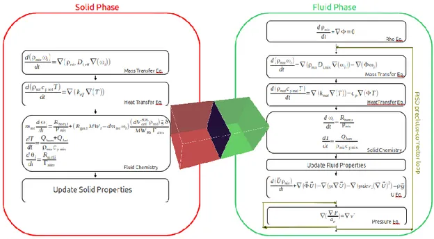
Fig. 3.6 -. Schematization of CatalyticFOAM-multiRegion solution procedure in the fluid and solid phase ... 62

Fig. 3.7 – Mesh separation for multiphase representation ... 64

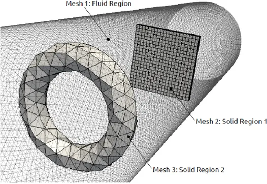
Fig. 3.8 – Example of mesh composed by three arbitrarily shaped regions ... 65

Fig. 3.9– polyMesh folder content after converting Gambit mesh to OpenFOAM format ... 67

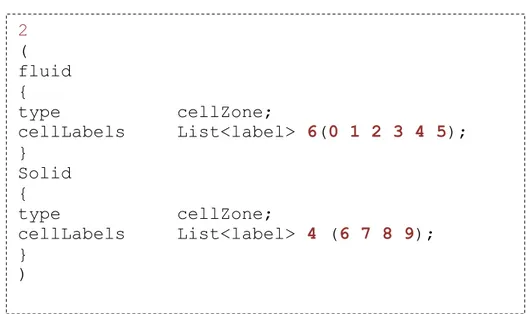
Fig. 3.10 – Example of cellZones file content ... 67

Fig. 3.11– Example of faceZones file content... 68

Fig. 3.13– Input folders 0, system, and constant in a multi-region case ... 69

Fig.3.14 – Example input file for concentrationCoupled and temperatureCoupled boundary type definition ... 72

Fig. 3.15 – Pimple loop representation ... 74

Fig. 3.16 – catalyticFOAM-multiRegion solver architecture ... 75

Fig. 4.1 – Pimple loop numerical structure for interface convergence ... 77

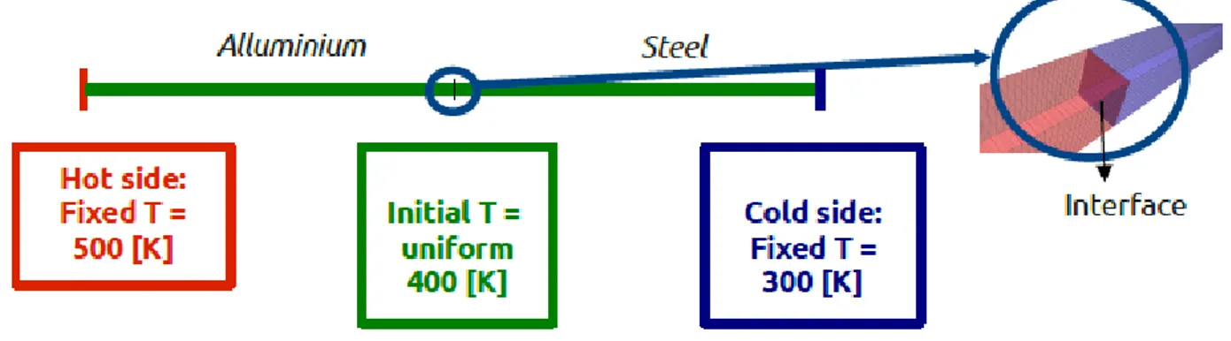
Fig. 4.2 – 1-D conjugate heat transfer: case presentation ... 78

Fig. 4.3– 1D schematization for temperature field ... 78

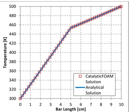
Fig. 4.4 – Comparison between solver and steady state analytical solution for heat transfer in 1D case... 80

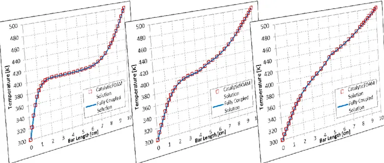
Fig. 4.5 – Comparison between fully coupled and catalyticFOAM solution in transient ... 81

Fig. 4.6 – 1D conjugate mass transfer: case presentation ... 82

Fig. 4.7– Conjugate mass transfer – comparison with steady state solution... 83

Figure 4.8 – Diffusion and reaction: case presentation ... 84

Fig. 4.9 – Diffusion and reaction: comparison with the analytical solution ... 85

Fig. 4.10 – Diffusion and reaction: comparison with the analytical solution ... 86

Fig 4.11 – Effect of time step in 1D case of diffusion and reaction ... 87

Fig 4.12– Effect of mesh refinement in 1D case of diffusion and reaction ... 88

Fig. 4.13– Chemical, diffusive and mass transfer regime at different operating conditions ... 89

(x axis: Slab Length *cm+ , y axis: CA *mol/m3+) ... 90

Fig. 4.14– Comparison between split catalyticFOAM-multiRegion solver and coupled MATLAB® solver for diffusion and reaction in 1-D system for a wide variety of conditions. ... 90

Fig. 4.15- 1-D case with diffusion and reaction using complex kinetic schemes ... 91

Fig. 4.16 – two 2D channels: case setup and description ... 92

Fig. 4.17– Two 2D channels: velocity field development in the channels ... 93

Fig. 4.18a – Two 2D channels: massive fractions reactant profiles inside the solid catalytic phase . 94 Fig. 4.18b – two 2D channels: massive fractions product profiles inside the solid catalytic phase .. 94

Fig. 4.19 – Channel with catalytic solid particle: mesh used for the simulation ... 95

Fig. 4.20b – 2-D case: fully developed velocity profile before the obstacle ... 96

Fig. 4.21a – 2-D case: H2 mass fraction map in the channel ... 97

Fig. 4.21b – 2-D case: H2O mass fraction map in the channel ... 97

Fig. 4.22 – 2-D case: mass fractions profiles of reactant and products along the flow coordinate x 98 Fig. 4.23 – 2-D case: mass fractions profiles of reactant and products along the radial coordinate y ... 98 Fig. 4.24 - Physical interpretation of the two predictor-corrector routines (Goisis and Osio 2011) . 99

Fig. 4.25a – Annular reactor ... 100

Fig. 4.25b – 1D diffusion with reaction case ... 100

Fig. 5.1 - Sketch of the annular catalytic reactor, adapted from (Maestri, Beretta et al. 2008). ... 103

Fig. 5.2 - 2D mesh used for the numerical simulation. ... 105

Figure 5.4 a-b. Conversion of O2 vs. temperature at flow rate of 0.274 Nl/min and 0.578 Nl/min. 107 Fig. 5.7 - Activity of the catalytic bed vs. axial reactor length. ... 111

Fig. 5.8 - O2 conversion vs. temperature for different catalytic bed at 0.274Nl/min. ... 111

Fig. 5.9 - O2 mass fraction along radial reactor direction in the solid phase at different temperatures ... 113

Figure 5.10 - O2 mass fraction along radial reactor direction at different temperatures ... 114

Fig. 5.11 - Velocity magnitude *m s-1+profiles at 523.15 K at 60 ms. ... 115

Fig. 5.12 - O2 mass fraction profiles at 0, 2 and 15 ms at 523.15 K. ... 115

Fig. 5.13 - O2 mass fraction profiles at 60 ms at 523.15 K in the catalytic layer. ... 116

Fig. 5.14 – H2O mass fraction profiles at 60, 100 ms and Steady State at 523.15 K in solid phase 116 Fig. 5.15 – H2O mass fraction profiles at 523.15 K in the catalytic layer ... 117

Tables Index

Table 3.1 - Expressions for the effective diffusivity ... 36

Table 4.1 – Norm-2 of the errors between fully coupled and split solution ... 87

Table 4.2 – Norm-2 of the errors between fully coupled and split solution ... 88

Chapter 1

Introduction

1.1 Motivation

The reactor is the heart of the chemical process, and a thorough understanding of the phenomena occurring during the transformation of reactants into the desired products is of vital importance for the development and optimization of the entire process. It is thus essential to have a deep knowledge of the fundamental parameters critical to chemical reactor design, such as reactor sizing and optimal operating conditions.

Catalytic reactions and reactors have widespread applications in the production of chemicals in bulk, petroleum and petrochemicals, pharmaceuticals, specialty chemicals, etc. The simultaneous developments in catalysis and reaction engineering in 1930s and 1940s acted as a driving force for the onset of rational design of catalytic reactors. These detailed design efforts, firmly based on sound mathematical principles, in turn triggered the development of several profitable catalytic processes. Various authors studied the engineering aspects of diffusion mass transport and reaction rate interaction. In particular, Thiele explained the fractional reduction in catalyst particle

activity due to intra-particle mass transfer limitations and proposed the concept of effectiveness factor reflecting the extent of utilization of the catalyst pellet (Thiele, E.W. 1939).

On the other hand, another simplification usually considered in catalytic reactors models is the uniform temperature inside the solid particle, which means a complete neglect of heat transfer limitations.

The main aim of this work is to get a more accurate description of the physical domain through a detailed description of heat and mass transfer inside the solid domain, which can be crucial in some systems, as well as of inter-phase transport phenomena between the solid and fluid phase. In this way, thanks to the simulation of the actual physics of the system, it is possible to get rid of most of the restrictive approximations often introduced, related to simplified forms of governing equations or specific geometries.

1.2 General overview

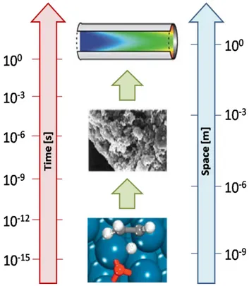
Without any doubts, one of the main difficulties encountered in the numerical modeling of the catalytic reactors is the great gap of different time and length scales involved, since the dominant reaction pathway is the result of the interplay between micro-, meso- and macro-scale phenomena (Figure 1.1).

Fig. 1.1 - Time and length scales involved in heterogeneous catalytic processes.

The microscopic scale is associated with making and breaking of chemical bonds between atoms and molecules. At the mesoscale the interplay between all the elementary steps involved in the catalytic process determines the main reaction pathway. At the macroscopic scale the transport of mass, energy and momentum determines local composition, temperature and pressure.

This means that the dominant reaction mechanism is a multi-scale property of the system (Maestri 2011). The description of different phenomena is achieved by employing a “first principles approach”, i.e. at each scale the fundamental governing equations are used. In particular:

 at the molecular scale the behavior of the system is described through detailed kinetic models, whose parameters are computed via first-principles electronic-structure calculations;

 at the meso-scale statistical methods give a rigorous representation of mechanisms taking place at the catalytic surface. Anyway the most common approach used in literature is the mean field approximation (Vlachos, Stamatakis et al. 2011). This approach assumes a perfect and rapid mixing of reactants, products, and intermediates on the surface;

 at the macro-scale methods based on continuum approximation are employed, e.g. resolution of Navier-Stokes equations with Computational Fluid Dynamics (CFD) (Reuter 2009).

Such a fundamental approach implies the development of efficient methodologies to connect the fundamental aspects across all the scales involved and link them in one multi-scale simulation.

Unluckily, the resulting numerical problem places highly computational demands mainly related to:

 the dimensions of the system are proportional to the number of species involved in the reacting process. Therefore, the more detailed the kinetic scheme is, the higher the required time is;

 ta proper discretization of the geometric domain is required to solve the problem. The number of cells in which the volume is divided is proportional to the accuracy and to the dimensions of the problem;

 the problem is very stiff because of the difference among the characteristic times and the characteristic lenghts;

 the presence of a reacting term implies a strong non-linearity of the governing equations. Furthermore, an accurate description of the problem should include a characterization of the catalytic phase and model intra-solid phenomena constituting the true nature of the diffusion-reaction mechanism. This acquires particular importance, especially when dealing with systems where heat and mass transfer limitations play a major role in determining the conditions holding on the catalytic surface. In these cases, neglecting the catalyst morphology can have a critical impact on the description of the system.

In the following, a summary on the most interesting approaches to these problems available in literature is provided.

1.3 State of the Art

The development of tools capable to describe the actual behavior of catalytic systems via first principles and multi-scale approaches is still in the initial phase. This is due to the complexity of the numerical problem that one has to handle. Recent advances in this field are owed to the vast diffusion of CFD applications.

Nowadays CFD is able to predict very complex flow fields due to the recent development of numerical algorithms and the availability of more performing computer hardware. However, CFD still lacks in the efficient handling of detailed kinetic schemes, mainly due to the difficult management of the huge number of reactions and species involved and to the stiffness of the resulting equations.

Recently the attention has been focused on the development of tools that implement heterogeneous kinetic models. In this section the most recent and challenging studies on coupling of microkinetic modeling and CFD are provided.

The most noticeable advances in this framework have been provided by (Deutschmann, Tischer et al. 2008) with the development of the DETCHEMTM software. This is a FORTRAN based collection of softwares designed to couple detailed chemistry models and CFD. The software package contains tools able to simulate time dependent gas-phase systems, with homogeneous gas-phase and/or heterogeneous surface chemical reactions. The list of tools contained in the DETCHEM library is presented below, together with mathematical aspects and range of applicability (Deutschmann, Tischer et al. 2011):

 DETCHEMBATCH and DETCHEMCSTR are computational tools that simulate homogeneous and heterogeneous reactions taking place respectively in a batch and CSTR reactor;

 DETCHEMPLUG is an application able to simulate the behavior of plug flow chemical reactors for gas mixtures. The model is mono-dimensional and it has been developed in the assumption of negligible axial diffusion and absence of variations in transverse direction;

 DETCHEMPACKEDBED is a tool for the simulations of packed bed reactors. The model is one-dimensional heterogeneous and assumes that there is no axial diffusion and no radial variations in the flow properties;

 DETCHEMCHANNEL is a computational tool that simulates the steady state chemically reacting gas flow through cylindrical channels using the boundary-layer approximation;

 DETCHEMMONOLITH is a simulation code that is designed to simulate transient problems of monolithic reactors, used whenever the interactions of chemistry, transport and reactor properties shall be investigated in monolithic structures of straight channels. It is assumed that there is no gas exchange between the channels and that the residence time of the gas inside the channels is small compared with the response time scale of the monolith. Furthermore, it is assumed that the cross-section of the monolith does not change along the channel axis;

 DETCHEMRESERVOIR is an application that allows to simulate isothermal transient behavior of monolith reactors. Only selected surface concentrations are assumed to vary over time (storage concentrations). The used approach consists in iterating steady-state and transient calculations. For each time step the DETCHEMCHANNEL or DETCHEMPLUG routines are called. The obtained steady-state values are then used by DETCHEMRESERVOIR as initial values in the integrations of site conservation balances of storage species;

 DC4FLUENT is a collection of user defined functions and works by coupling the DETCHEM routine with the commercial CFD code FLUENT. Furthermore the routines of the DETCHEM library are used to calculate source terms for the governing equations of mass, species and energy by the DC4FLUENT plugin.

As regards solid volume description, DETCHEMTM provides two different models: (i) a simple model, which is based on the concept of effectiveness factors, and (ii) a detailed approach, which is based on solving reaction-diffusion equations within the solid volume. The former is a very fast model, but it introduces a strong simplification; the latter is a time consuming model because it solves the reaction-diffusion equations for every species within the solid volume.

The studies that have been developed by using this software package are presented in the following.

In (Deutschmann, Correa et al. 2003) the start-up of the catalytic partial oxidation (CPO) of methane over rhodium/alumina in a short contact times reactor was investigated. The study was conducted by employing the DETCHEMMONOLITH code. The triangular shape of the single channel of the monolith was approximated with a cylindrical structure. Five representative channels were simulated in order to describe the behavior of the monolith. The kinetic scheme adopted comprehends both gas-phase and surface reaction mechanism.

A study on the abatement of automotive exhaust gases on platinum catalysts was performed by (Koop and Deutschmann 2009), by using the DETCHEMCHANNEL application. The two-dimensional flow-field has been described and a detailed reaction mechanism for the conversion of CO, CH4,

C3H6, H2, O2 and NOx has been included. Based upon experiments with a platinum catalyst in an

isothermal flat bed reactor, a detailed surface reaction mechanism has been developed. Numerical simulations of the thermodynamic equilibrium of nitrogen oxides and calculations of surface coverage on platinum have been performed.

Mladenov and co-workers (Mladenov 2010) performed a CFD study in order to understand the impact of the real wash-coat shape on the overall reaction rate. The computational tools used from the DETCHEM package are DETCHEMCHANNEL and DC4FLUENT plugin. The aim of the work was to study mass transfer in single channels of a honeycomb-type automotive catalytic converter operated under direct oxidation conditions. Specifically, 1D, 2D and 3D simulations were performed on channels of different shapes, respectively circular cross section, square cross section and square cross section with rounded corners. Furthermore, the effect of diffusion in a porous wash-coat was investigated. The reaction mechanism comprehends 74 reactions among 11 gas-phase and 22 adsorbed surface species.

An example of multiphase CFD with reactionis performed in a study by Tischer et al. (Tischer et al., 2007), where a PDEX (Nowak et al. 1996) 1D transient Model of Gas Flow and Temperature Profile is compared with a DetchemTM solver for the simulation of a three-way catalyst. Although DETCHEM is also capable of surface reaction mechanisms simulation, the same global-step reaction mechanism was used in order to make kinetics consistent. As regards the solid phase description, instead of including the diffusion limitations of the wash-coat through an efficiency factor for the reaction, DETCHEMTM makes use of a wash-coat diffusion sub-model in order to describe the influence of the wash-coat thickness. Finally the DETCHEMTM results were compared with experimental data.

Beside these works developed with the DETCHEM library, another interesting study has been realized by Vlachos and co-workers (Vlachos, Kaisare et al. 2008). They performed a study on catalytic combustion of propane on platinum in micro-reactors under laminar conditions. A comprehensive parametric analysis was made investigating the role of inlet velocity, equivalence ratio and reactor size. A two-dimensional model was used. The kinetic model adopted consisted of

a one-step reaction mechanism, obtained via a-posteriori model reduction of detailed microkinetic mechanism.

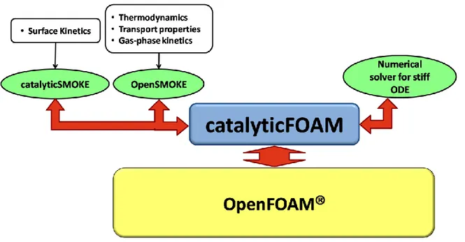
An interesting work, aiming at considering all the scales involved in catalytic reactors, has been made by (Goisis and Osio 2011) where a CFD solver has been built up in the OpenFOAM® (OpenFOAM® 2011) framework, an open source CFD code. Its characteristics are summarized below:

 it can handle detailed kinetic mechanisms without any constraint on the number of species and reactions involved. The microkinetic description is provided by the CatalyticSMOKE libraries (Goisis and Osio 2011). These adopt standard CHEMKIN (ReactionsDesign 2008) correlations and can handle both classical and UBI kinetic schemes (Maestri and Reuter 2011, Goisis and Osio 2011);

 good efficiency in handling multi-scale coupling thanks to the splitting operator method, which solves the main problem (PDEs system, stiff, non-linear and fully coupled) through the solution of two sub-problems: the chemical reaction (a coupled, non-linear and stiff system of ODEs) and the transport (a decoupled, quasi linear, non-stiff system of PDEs ). In this way the problem can be efficiently solved (Strang 1968; Pope and Zhuyin 2008);

 solution of the Navier-Stokes equations with the Pressure Implicit Splitting Operator (PISO) (Issa 1986) method;

 no limitations in the shape of the geometric domain: any three-dimensional domain can be investigated. If the system has specific symmetry properties, it can be studied with a 2D simulation, saving a considerable amount of time (Goisis and Osio, 2011).

A missing feature in the mentioned work is the detailed description of the phenomena occurring inside the catalytic phase, leading to a multi-region approach to the problem. This is one of the main breakthroughs developed in this thesis. The implementation of this feature inside the OpenFOAM® framework is still debated within the Open Source community, where two different approaches have been proposed:

 monolithic: this approach involves a single coupled system of equations on a single matrix taking into account both the phases involved. When dealing with multiple regions with different properties, this approach can work just for loose inter-equation coupling (Clifford 2011). Furthermore, the management of the constitutive equations, the storage of field

variables and all post-processing operations would become harder with a single matrix approach;

 partitioned: this approach involves governing equations solved separately on each of the coupled regions, imposing appropriate boundary conditions on both ends. To make the coupling effective, the procedure must be iterated until convergence is reached (Craven and

Campbell 2011). If this can be seen as a negative aspect in terms of computational time, the

advantage of this approach is that it works on multiple meshes even for stiff inter-equation coupling.

The latter approach has been adopted in this work in order to avoid all the approximations usually introduced when modeling the catalytic pellets and, instead, to simulate the reaction environment (both solid and fluid) with equations describing the actual physics of the system.

Furthermore, it is important to consider that in general real systems present different diffusivities for different materials, and it is important to take into account for effective properties in the different solid phase domains considered accordingly.

Another phenomenon which can be crucial for a correct model of a real system is the heat conduction and heat transfer limitations in the solid phase. The correct modeling of heat exchange phenomena makes it possible to predict the temperature in any point of the solid domain and, as a consequence, to get a numerical estimation of the catalyst activity and to identify hotspots in the reactor design.

Of course, besides working in a reacting environment, the tool proposed can also be used to simulate simpler non-reacting multi-region systems, such as heat exchangers, or complex systems composed of reacting regions and non-reacting ones.

The methodologies followed in this work to accomplish these objectives are explained in the next paragraph.

1.4 Methodologies and main results

The tool developed in this work, named catalyticFOAM-multiRegion, was built up in the OpenFOAM framework (OpenFOAM® 2011), an open source CFD code.

As extensively stated in the previous sections, the main aim of this solver is to model in detail both the solid and the fluid phases of catalytic reactors, through the resolution of the fundamentals equations describing the physics of the system in each phase. The tools available for the implementation are the OpenFOAM® libraries, able to handle variable fields in order to dynamically describe the system, and kinetic libraries, giving the solver the possibility to simulate complex kinetic schemes. An accurate description of the physical problem and the mathematical model developed to describe the system, together with an insight on the tools used for the development, are provided in Chapter 2.

The available CFD tools that solve this class of heterogeneous reacting problems have large difficulties in handling multi-scale coupling efficiently. On one side, fully coupled methods are suitable only for problems of small dimensions. On the other side, segregated methods are inappropriate for the solution of stiff and non-linear problems. To overcome these difficulties a new approach based on the splitting operator method has been proposed (Goisis and Osio, 2011). This allows to split the problem in two sub-problems and to solve them decoupled. In Figure 1.2 a schematization of the splitting operator method is presented.

This implies the following advantages:

 possibility to select the best numerical algorithm for each sub-problem;  stiffness and non-linearity are enclosed only in one sub-problem;

 low stiffness and quasi-linearity permit to adopt a fully segregated approach in the transport step.

Consequently the problem can be efficiently solved (Strang 1968; Pope and Zhuyin 2008).

The application of a splitting operator scheme to our problem has been achieved by separating the portions of the governing equations containing chemical reaction terms from those containing the transport terms. The latter are solved in sequence, each one decoupled from the others, as prescribed by the segregated approach. Instead of having a huge system of PDEs, one has to solve each equation of the system decoupled. A special attention has to be paid to the Navier-Stokes equations. Indeed, the strong coupling with the continuity equation makes it necessary to treat the inter-equation coupling in an explicit manner. The procedure followed is the Pressure Implicit Splitting Operator (PISO) method (Issa 1986). PISO and their derivatives are the most popular methods for dealing with inter-equation coupling in the pressure-velocity system for transient solutions (Jasak 1996). In addition to that, to handle multiple regions and their interaction, a partitioned approach is adopted: governing equations are solved separately on each of the coupled regions, imposing appropriate boundary conditions (mixed boundary conditions) at the interface between two different phases. To make the coupling effective, the procedure must be iterated until convergence is reached (PIMPLE Loop). Further information about the numerical strategies adopted throughout the solver, as well as the final architecture of the solver for both the description of intra-phase phenomena and inter-phase phenomena occurring at coupled interfaces, can be found in Chapter 3.

The application of these methodologies led to the development of the catalyticFOAM-multiRegion solver. The work was mainly focused on the implementation of the code. This was made by adding one feature at a time and validating it before proceeding. The main features of this tool are:

 the possibility to solve homogeneous reacting flows in the fluid zones and both homogeneous and heterogeneous reacting flows in the solid zones;

 the ability to perform simulations with an accurate description of the velocity field by the resolution of the Navier-Stokes equations in both laminar and turbulent conditions, with any arbitrary geometric domain;

 the possibility to solve heat conduction problems and to model adiabatic or isothermal systems;

 the possibility to describe the reaction mechanisms with detailed kinetic models;

 the capability to handle an arbitrary number of different regions and phases, each with its own properties and meshed separately;

 the attribution of distinct governing equations and properties on each region;

 the physical sound description of intra-solid heat and mass transfer phenomena, making possible to account for diffusive limitations inside the catalytic phase;

 the effective description of conjugate heat-mass transfer inter-phase phenomena through the implementation of new libraries managing coupling boundary conditions at the interface

All the features described above are tested in Chapter 4, performing numerical tests on different parts of the solver architecture by approaching test cases of increasing complexity, in order to prove the validity and effectiveness of the segregated numerical approach proposed for both inter-phase coupling and intra-inter-phase phenomena description in both the fluid and the solid inter-phase. The solver solution has been compared to analytical or numerical, fully-coupled solutions when possible.

Finally, in order to investigate the reliability of the solver, a validation has been performed in Chapter 5. The fuel-rich H2 combustion over Rh catalyst in an annular reactor has been analyzed

and the simulation results have been compared with experimental data. Specifically, data on oxygen conversion achieved in the reactor at different temperatures have been compared with isothermal simulations performed with the solver developed in this work. In particular, the attention has been focused on the temperature range where previous works (Maestri et al. 2008, Goisis and Osio 2011) over-estimated oxygen conversion and were not able to reproduce the experimental data properly, due to the lack of description of intra-phase phenomena inside the solid phase. Thanks to its capability to reproduce the physics of both inter-phase interaction and intra-phase phenomena inside the solid catalyst, the developed tool provides a satisfactory fit with

experimental data in these temperature ranges, describing accurately concentration profiles inside the solid phase and being thus able to represent both chemical controlled regime and mass-transfer controlled regime.

Chapter 2

Physical Problem and Computational Tools Available

In this chapter, we first describe the physical problem we aim to solve, which is the generic catalytic reacting system, and the mathematical model used to describe this system, after introducing the solid phase and its characterization. Secondly, we briefly describe the main tools that will be used in order to develop and build the solver: the OpenFOAM® framework, and the OpenSMOKE and catalyticSMOKE kinetic libraries.

2.1 Physical problem and mathematical model

The aim of the work herein presented is the detailed description of gas-solid catalytic reactors. In order to properly model this system, it is necessary to address different phenomena, such as heat and mass transfer occurring both in the gas and solid phase (intra-phase phenomena) and between them (inter-phase phenomena), the velocity and pressure fields due to the fluid flow in the reactor, and the gas-phase and surface reactivity.

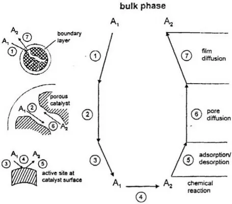
The most important phenomena taking place in a catalytic reaction can be summarized as shown in Fig. 2.1:

Fig. 2.1 – Individual steps of a simple, heterogeneous catalytic fluid-solid reaction A1->A2 carried out on a

porous catalyst (Bird,Stewart, Lightfoot 2002)

1) film diffusion: the reactants diffuse from the bulk phase to the boundary layer surrounding the solid phase;

2) pore diffusion: the reactants diffuse from the boundary layer to the solid phase through the catalyst pores;

3) adsorption: the reactants physically or chemically adsorb on the solid surface. If the adsorption is chemical, a free active site is necessary for the adsorption to take place;

4) surface reaction: the adsorbed species react between each other or with gas-phase species;

5) desorption: the reaction products desorb from the catalytic surface;

6) pores back-diffusion: the reaction products diffuse from inside the catalyst to the boundary layer surrounding the solid;

7) film back-diffusion: the reaction products diffuse from the boundary layer to the bulk.

Moreover heat transfer phenomena are associated with this steps and need to be considered.

In a previous work (Goisis and Osio 2011) the attention was focused on the interplay between the Navier-Stokes equation and the surface reactivity based on a micro-kinetic description of the

surface reactivity. Nevertheless, intra-phase mass and energy phenomena inside the catalyst were neglected. The aim of this work is to describe in detail every single phase mentioned above, in order to fully account for diffusive limitations and phenomena occurring inside the catalytic solid itself.

Beside the wide variety of different reactors which can be found in reality, their description is not based on the external form of the apparatus nor on the reaction taking place in it, nor even on the nature of the medium-homogeneous or not. The phenomena occurring in a reactor may be broken down to reaction, transfer of mass, heat, and momentum. The modeling and design of reactors is therefore based on the equations describing the previously listed phenomena:

- the continuity equation - the momentum equation - the energy equation

- the species transport equation

The solution of these equations will provide a full characterization of the system in terms of its main variables for each phase considered:

- Velocity

- Pressure

- Density

- Temperature

- Gas species concentrations

- Adsorbed species concentrations

The form and complexity of the mathematical model dealing with these equations will be discussed in 2.1.2, while in 2.1.1 a deeper description of the solid phase is given.

2.1.1 The introduction of the solid phase

2.1.1.1 The need for fluid and solid cells

In a previous work (Goisis and Osio 2011) the catalyst morphology was not detailed, and the presence of that phase was taken into account by endowing the cells close to the catalytic layer itself with an additional heterogeneous reactive term and a boundary condition imposing continuity between the reactive flux and the diffusive flux to and from the catalytic surface. As discussed previously, this approach was not capable of taking into account diffusive limitations in the solid phase or in general intra-solid transport phenomena occurring there. In this work, a new approach has been developed, capable of taking into account both the phenomena occurring in the fluid and in the catalytic solid phases.

Fig. 2.2 - Fluid and solid cells schematization

Aim of this work is thus to provide a tool capable of describing both the inter-phase and the intra-phase phenomena occurring in both the fluid and solid intra-phase of a catalytic reactor. In particular,

the latter has been considered as a porous pseudo-homogeneous phase, including both the solid catalytic surface and the fluid contained inside its pores, as shown in Figure 2.2.

Thus, two different types of cell zones have been accounted for in the solver: (i) the “homogeneous” cells, which contain only the gas phase reactions, and (ii) the “catalytic” cells, which involve the heterogeneous reactions. In the following only heterogeneous phenomena have been considered to take place in catalytic cells, as the low gaseous volumes present in the solid pores and the presence of the catalytic surface inhibit heavily homogeneous reactions occurring in the gas phase inside the catalyst pores.

2.1.1.2 Catalytic solid phase characterization

As regards the physical characterization of the catalytic cells, properties are considered to be uniform in every portion of the catalytic volume. The main parameters used to describe the catalyst morphology embedded into the model are:

 the void fraction ε, representing the volume of voids over the total volume of the cell, allowing the gaseous phase inside the pores to be taken into consideration;

 the effective catalytic surface per unit of volume 𝑎𝑐𝑎𝑡 , which can be often found in the

literature as a characteristic parameter of a catalytic geometry.

When this parameter is not known, it is still possible to estimate it if other physical properties of the catalyst are available. For example, in the case of supported catalysts, it is possible to compute it as:

𝑎𝑐𝑎𝑡 =

𝑊_𝑐𝑎𝑡∙ ξ ∙ δ MWRh ∙ Γsites ∙ V

(2.1)

where ξ is the fraction of the active phase over the total catalyst mass *kgActive/kgCat+, δ is the

fraction of active sites available over the total active sites *molAvailableAct/molTotAct+, Γsites is the

2.1.2 Mathematical Model

As mentioned at the beginning of this chapter, the most general equations to represent the physics of the system to be modeled are the equations of continuity, momentum, energy, and species (gaseous and adsorbed). In this paragraph it will be shown how these conditions have been implemented into a mathematical model, with the aim of describing the whole range of phenomena occurring in both the fluid and the solid catalyst.

2.1.2.1 Navier-Stokes Equations

For a correct description of the flow field it is necessary to solve the Navier-Stokes equations for the momentum transport under the hypothesis of Newtonian fluids:

𝜕(𝜌𝑼)

𝜕𝑡

+ 𝛻(𝜌𝑼𝑼) = −𝛻𝑝 + 𝛻(𝜇𝛻𝑼) + 𝜌𝒈

where µ is the dynamic viscosity, g is the gravity acceleration, 𝑼 is the velocity vector, ρ is fluid mixture density and p is the pressure.

Being the density field interconnected with the velocity and pressure fields, it is necessary to add the continuity equation:

𝜕𝜌

𝜕𝑡

+ ∇(𝜌𝑼) = 0

For compressible fluids it is requested the knowledge of the pressure field, described by the equation of state. Since the technological interest is focused on processes where the flowing phase is gaseous, the ideal gas approximation is adopted:

𝜌 =

𝑝𝑀𝑊

𝑅 𝑇

where MW is the molecular weight and R is the universal gas constant.

2.1.2.2 Species transport equation

As we want to consider multicomponent mixtures, we solve the transport equation of species under the hypothesis of Fickian diffusion, as follows:

𝜕(𝜌𝜔

)

𝜕𝑡

+ ∇(𝜌𝑼𝜔

) = ∇(ρ𝐷

∇𝜔

) + ∑ 𝑅

𝜈

𝑀𝑊

Di represents the mass diffusivity of the ith species in the reacting mixture and υij is the

stoichiometric coefficient of the ith species in the jth reaction. Rj is the rate of the jth reaction.

2.1.2.3 Energy trasport equation

In order to describe the temperature field, the solution of the energy balance is required.

𝑐

𝜕(𝜌𝑇)

𝜕𝑡

+ 𝑐

∇(𝜌𝑼𝑇) = ∇(k∇T) + ∑ 𝑅

∆𝐻

where T is the temperature, Cp is the specific heat of the gas mixture and ΔHj is the heat of

reaction of the jth reaction. The energy dissipation due to the viscosity of the fluid is neglected. Furthermore, the pressure term can be ignored (Bird 2002).

2.1.2.4 Transport equations in the solid phase

When considering the solid phase, the equations previously shown will have slight differences related mainly to the absence of flow through the solid phase. In the latter, in fact, a diffusion and reaction model will be considered:

 there is no need to solve the Navier-Stokes equation in the solid phase, in the hypothesis of absence of flow through the catalytic solid pores;

 in the heat and mass transfer equations, for the same reason, no convective term has been considered (respectively ∇(𝜌𝑼𝜔𝑖) and 𝑐𝑝∇(𝜌𝑼𝑇) shown in the equations above). The

resulting equations for species and energy transport in the solid phase are then:

𝜕(𝜌

𝜔

)

𝜕𝑡

= ∇(𝜌

𝐷

∇𝜔

) + ∑ 𝑅

𝜈

𝑀𝑊

𝜕(

𝑇)

𝜕𝑡

= ∇

∇T

+

𝑅

∆𝐻

where ωi is the mass fraction of the ith component, 𝐷𝑒𝑓𝑓,𝑖 and λ𝑒𝑓𝑓 represents the effective

diffusivity of the ith species and effective conductivity, 𝜌𝑠𝑜𝑙 and 𝜌𝑚𝑖𝑥 are respectively the apparent

density of the solid phase and density of the gas phase inside the catalyst pores, νij is the

stoichiometric coefficient of the ith species in the jth reaction. Rj is the rate of the jth reaction and

includes both homogeneous and heterogeneous reactions.

2.1.2.5 Effective properties in the solid phase

The means to predict mass and heat transport of gases in porous solids in present days are inaccurate as a consequence of the inherent difficulties encountered in properly relating the local transport coefficients to the highly complex pore space. Due to the complexity of the catalysts morphology, the solid phase has been characterized with effective properties uniform in the whole catalytic volume, as already widely done in literature. The effective diffusivity inside the solid phase has been espressed as a function of the diffusivity computed in the gaseous bulk phase through a reduction factor, making it possible to take into account for transport limitations in the catalytic phase and incomplete use of the catalyst volume:

𝑘𝑑𝑖𝑓𝑓𝑢𝑠𝑖𝑣𝑖𝑡𝑦 =

𝐷_{𝑠𝑜𝑙𝑖𝑑} 𝐷𝑏𝑢𝑙𝑘

(2.8)

When this parameter is not known from experimental measurements, such as mercury penetration methods (Kim,Ochoa et al. 1987), it is still possible to obtain it from catalyst porosity values with predictive models based on experimental measures (Mezedur, Kaviany et al. 2002) or on random porous solid 3-D models capable of taking into account micro-morphology features such as pore sizes, pore orientations, interconnections, dead ends, etc. (Mu,Liu et al. 2007).

Here below an example of the expressions which can be found in the literature is reported (Mu,Liu et al. 2007) : 𝐷𝑒𝑓𝑓 𝐷_{𝑏𝑢𝑙𝑘} = 2𝜀 3 − 𝜀 𝐷𝑒𝑓𝑓 𝐷_{𝑏𝑢𝑙𝑘} = 𝜀1.5 𝐷𝑒𝑓𝑓 𝐷𝑏𝑢𝑙𝑘

=

= 1 − (1 − 𝜀)

Table 3.1 - Expressions for the effective diffusivity

Another effective property of the solid phase which has been considered in the mathematical model is the effective conductivityλ𝑒𝑓𝑓, which needs to be evaluated through predictive models or

experimental measurements.

2.1.2.6 Reactive term in different phases

In order to model properly the multiphase system, it is necessary to mathematically describe all the phenomena taking place both in the solid and in the fluid phase. All the species can:

 lead to homogeneous reactions in the fluid phase;  diffuse from the fluid to the solid phase and vice-versa. Once inside the solid phase, reactants can

 adsorb on the catalytic surface and lead to heterogeneous reactions;  react in the fluid phase inside the solid pores.

As previously stated, homogeneous reactions taking place inside the catalyst pores will be reasonably neglected. Naturally, the reaction creates a concentration gradient which makes new reactants move from the fluid to the solid phase until a steady state is reached, and all the reactions will be accompanied by heat generation.

Now that the solid phase has been characterized, it is possible to write again the mathematical model described in the previous paragraph, detailing the reactive terms which have not been

detailed yet. These equations express species and heat transport and generation due to the reaction, and their derivations are provided in Appendix A.

 In the homogeneous phase:

{ 𝜕(𝜌𝜔𝑖) 𝜕𝑡 + ∇(𝜌𝑼𝜔𝑖) = ∇(ρ𝐷𝑖∇𝜔𝑖) + ∑ 𝑅𝑗 ℎ𝑜𝑚,𝑗𝜈𝑖𝑗𝑀𝑊𝑖 𝑐_𝑝𝜕(𝜌𝑇) 𝜕𝑡 + 𝑐𝑝∇(𝜌𝑼𝑇) = ∇(k∇(T)) + ∑ 𝑅𝑗 𝑗∆𝐻𝑗 (2.9)

 In the heterogeneous phase cells, on the other hand:

{ 𝜕(ρ𝑚𝑖𝑥𝜔𝑖) 𝜕𝑡 = ∇(ρ𝑚𝑖𝑥𝐷𝑒𝑓𝑓,𝑖∇𝜔𝑖) + (∑ 𝑅𝑗 ℎ𝑒𝑡,𝑗𝜈𝑖𝑗𝑀𝑊𝑖) ∙ 𝑎𝑐𝑎𝑡 𝑐_{𝑝,𝑠𝑜𝑙}𝜕(𝜌𝑠𝑜𝑙𝑇) 𝜕𝑡 = ∇(k𝑒𝑓𝑓∇T) + ∑ 𝑅𝑗 ℎ𝑒𝑡,𝑗∆𝐻𝑗 ∙ 𝑎𝑐𝑎𝑡 (2.10)

where Rhom,i is the homogeneous reaction rate for the i-th specie 𝑖𝑛 [ 𝑘𝑚𝑜𝑙_𝑖

𝑚_{𝑟𝑒𝑎𝑡𝑡}3 𝑠] and Rhet,i is the

heterogeneous surface reaction rate in [_𝑚𝑘𝑚𝑜𝑙𝑖

𝐶𝐴𝑇2 𝑠] , which needs to be multiplied by the specific catalytic area 𝑎_𝑐𝑎𝑡 [ 𝑚𝐶𝐴𝑇2

𝑚_{𝑅𝐸𝐴𝑇𝑇}3 +. As regards the properties of the solid, 𝐷𝑒𝑓𝑓,𝑖and λ𝑒𝑓𝑓 are the effective

properties of the catalytic pseudo-phase, as described in the previous paragraph.

Furthermore, site conservation balances have to be written as follows:

Γ𝑠𝑖𝑡𝑒

𝜕𝜗𝑖

𝜕𝑡 = 𝑅𝑖,𝑠𝑢𝑟𝑓 (2.11)

where θi is the site fraction of the ith species and Γ𝑠𝑖𝑡𝑒 is the sites density and 𝑅𝑖,𝑠𝑢𝑟 is the

production rate of the ith surface species.

After presenting the mathematical model adopted, it is necessary to address the numerical issues related to its solution and to develop a solver which can handle the computational structure defined. This has been done in Chapter 3.

The model shown above results in a system of Partial Differential Equations (PDEs), which requires a computational tool in order to be solved. For its increasing popularity in the CFD community and its versatility, the OpenFOAM® framework has been chosen for this scope, and it will be briefly described in the next paragraph, together with the libraries adopted for the computation.

2.2 Tools available

2.2.1 OpenFOAM framework

2.2.1.1 General overview

The aim of this section is to introduce the main features of OpenFOAM as support code for CFD simulations and its practical use.

OpenFOAM is a C++ library created in 1993 and it is an object-oriented numerical simulation toolkit for continuum mechanics. Its popularity is increasing in the last years because OpenFOAM is released under General Public License (GPL), including the possibility to have at disposal the whole code and eventually modify it as needed. It is capable to support all the typical features of C++ programming, e.g. creation of new types of data specific for the problem to be solved, construction of data and operations into hierarchical classes, handling of a natural syntax for user defined classes (i.e. operator overloading) and it easily permits the code re-use for equivalent operations on different types (Mangani 2008).

OpenFOAM is not meant to be a ready-to-use software, even if it can be used as a standard simulation package. Rather, it offers a support in building user specific codes.

Like the widest part of CFD software, OpenFOAM provides tools not only for the finite volumes calculations, but also for pre and post processing. A schematic of the library structure is given in Figure 2.3.

Fig. 2.3 - OpenFOAM library structure (OpenFOAM user guide, 2011).

mesh, only with the corresponding initial and boundary conditions. Post-processing utilities allow one to view and analyze simulations results. The computational part is based on solvers, applications designed to solve specific classes of engineering problems, e.g. aerospace, mechanics, chemistry.

The latest OpenFOAM version (2.1.1) includes over 80 solver applications and over 170 utility applications that perform pre- and post-processing tasks, e.g. meshing, data visualization, etc. In the following we present the structure and organization of an OpenFOAM case. In general the sequence of work in OpenFOAM can be divided into three consecutive steps:

 pre-processing: firstly it is necessary to set-up the problem;

 processing: the simulation is performed by a solver;

 post-processing: results are displayed with specific application for data analysis and

manipulation.

Pre-processing

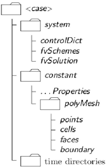
The basic directory structure for the set-up of an OpenFOAMcase is represented in Figure2.4.

Fig. 2.4 - Directory structure for the set-up of an OpenFOAM case.

The case folder includes:

The constant directory containing information about physical properties.

The time directories containing individual data files for each field (e.g. temperature, pressure, compositions) at different times of simulation.

The system directory for setting numerical parameters associated with the solution procedure.

It is necessary to pay great attention to the creation of the computational mesh in order to ensure a valid and accurate solution.

OpenFOAM provides a mesh generation utility called blockMesh that creates parametric meshes with specified grading and arbitrary curved edges. The mesh is generated from a dictionary file named blockMeshDict located in the constant/polyMesh directory. The utility reads this dictionary, generates the mesh and creates the mesh data.

In order to easily generate elaborate meshes it is possible to use a variety of software, such as

GAMBIT (Fluent 2004), a mesh generation software owned by Ansys FLUENT, which writes mesh

data to a single file. OpenFOAMprovides a tool for the conversion of GAMBIT meshes to the OpenFOAM format.

Initial and boundary conditions for a certain number of fields are required in order to start the simulation. These data are stored in the 0 folder: each file contains for every variable the initial conditions for the internal field and the declaration of each boundary condition. The latter has to be chosen from a list of pre-built standard conditions (OpenFOAM® 2012).

The system directory contains at least the following three files: controlDict, fvSchemes and fvSolution. In the first one run control parameters are set, including start/end time, time step and other specifications. The fvSchemes file contains the discretization schemes used in the solution. Typically one has to assign the discretization methods for gradient, divergence etc. In the fvSolution file algorithms for the solution of each equation are selected and tolerances for each variables are set.

Processing and post-processing

During the calculations the solver iterates the numerical procedure and periodically writes results at intermediate times. It is possible to choose how often taking note of the results (setting the

writeInterval = timeIntervalBetweenSuccessiveRecords in the

in the controlDictionary file). It is also possible to choose between two different format of writing files:

- writeFormat = BIN: faster writing operation, output files unreadable with text editor tool, but observable through sampling and plotting or classical post processing;

- writeFormat = ASCII: slower writing operation, output files readable with text editor tool as well as observable with more classical methods.

There are some tricks to make the simulations faster. For example it is possible to run a simplified and lightened form of the solver (simpleFoam) just to get the stationary field for velocities and take it as starting point: in this way the field variables involved in the Navier-Stokes equations are closer to their stationary value.

OpenFOAM is supplied with the post-processing utility ParaView (Ahrens, Geveci et al. 2005), an open source multi-platform data analysis and visualization application which provides a lot of useful tools for these scopes.

2.2.1.2 The math behind OpenFOAM

The widest part of complex engineering systems is described by one or more Partial Differential Equations (PDEs). Since the majority of these equations does not have an analytical solution, it is necessary to solve them with numerical methods (Quarteroni and Valli 1999).

In this paragraph the fundamentals of numerical procedures of discretization and solution are presented.

Discretization algorithm

The purpose of any discretization practice is to transform one or more PDEs into the resulting system of algebraic equations to allow the numerical solution. The discretization process consists of splitting of the computational domain into a finite number of discrete regions, called control volumes or cells. For transient simulations, it is also required to divide the time domain into a finite number of time-steps. Finally, it is necessary to re-write equations in a suitable discretized form.

The approach of discretization adopted by OpenFOAM is the Finite Volume Method (FVM) (Versteeg and Malalalsekera 1995). The main features of this method are listed below:

 the governing equations are discretized in the integral form;

 equations are solved in a fixed Cartesian coordinate system on the computational mesh. Solution can be evaluated both for steady-state and transient behaviors;

 the control volumes can have a generic polyhedral shape: together they form an un-structured mesh (Patankar and Spalding 1972; Van Doormaal and Raithby 1985).

In the following we provide a short description of discretization of domain, time and equations.

Domain discretization

The discretization via FVM entails the subdivision of the domain in control volumes or cells. These have to completely fill the domain without overlapping. The point in which variables are calculated is located in the centroid of the control volume of each cell, defined as:

∫ (𝒙 − 𝒙𝑷)𝑑𝑉 = 𝟎 𝑉𝑃

(2.12)

where 𝒙𝑷 stands for the coordinate of the centroid, as shown in Figure 2.3.

The domain faces can thus be divided in two classes: internal faces, between two control volumes, and boundary faces, which coincide with the boundaries of the domain. A simple example of domain discretization is showed in Figure 2.5.

Fig. 2.5 - Example of finite volume discretization (OpenFOAM® User guide, 2011).

In Figure 2.3 the point P and N represents the centroid of the cells of the geometric domain. The vector d represents the distance between the two centroids. The vector Sf is the surface vector outgoing from the generic flat face f.

Equations discretization

Let us consider the standard form of the transport equation of a generic scalar field φ:

𝜕(𝜌𝜙)

𝜕𝑡 + ∇(𝜌𝑼𝜙) − ∇(Γ∇𝜙) = 0 (2.13)

where 𝑼 is the velocity vector and Γ is the generic diffusion coefficient (e.g. thermal conductivity). For the sake of clarity the source term has been neglected. Further details on the discretization of the source term can be found in section 2.3.3.

The finite volume method requires that Eq. (2.14) is satisfied over the control volume VP in the

integral form: ∫ [𝜕 𝜕𝑡∫ 𝜌𝜙𝑑𝑉 + ∫ ∇ ∙ (𝜌𝑼𝜙)𝑑𝑉 − ∫ ∇ ∙ (𝜌Γ∇𝜙)𝑑𝑉_{𝑉𝑃 𝑉𝑃 𝑉𝑃} ] 𝑑𝑡 𝑡+∆𝑡 𝑡 = 0 (2.14)

The discretization of each term of Eq. (2.15) is achieved by applying the Gauss theorem in its general form:

∫ ∇𝜙𝑑𝑉 = ∮ 𝜙𝑑𝑆

𝜕𝑉 𝑉

(2.15)

Having in mind that each cell with volume V is bounded by a list of flat faces, it is possible to re-write the integral of Eq. (2.16) as a sum over all faces. The combination of Eq. (2.15) and (2.16) leads to:

(∇𝜙)𝑉_𝑃 = ∑ 𝑆_𝑓𝜙_𝑓

𝑓 (2.16)

where 𝑉𝑃 is the volume of the cell, Sf is the surface of the cell and 𝜙𝑓 is the flux of the generic

scalar 𝜙 through the face f.

Time discretization

In transient problems it is fundamental to adopt numerical methods to handle temporal integration. Let us consider the first term of Eq. (2.15):

∫ [𝜕

𝜕𝑡∫ 𝜌𝜙𝑑𝑉 +_𝑉 ∫ 𝛹(𝜙)𝑑𝑉_𝑉 ] 𝑑𝑡

𝑡+Δ𝑡

𝑡

(2.17)