Asian options on arithmetic and harmonic averages

FACOLTÀ DI SCIENZE MATEMATICHE, FISICHE E NATURALI Corso di Laurea Magistrale in Matematica

ASIAN OPTIONS ON ARITHMETIC

AND HARMONIC AVERAGES

Tesi di Laurea in Equazioni Differenziali Stocastiche

Relatore:

Chiar.mo Prof.

ANDREA PASCUCCI

Presentata da:

ANDREA FONTANA

III Sessione

Anno Accademico 2011/2012

INTRODUCTION 5

1 PRICES OF ASIAN OPTIONS 7

1.1 Preliminaries . . . 7

1.2 Approximation methodology . . . 12

2 ARITHMETIC AVERAGE 19 2.1 Explicit first order computation . . . 19

2.2 Numeric results . . . 36

3 HARMONIC AVERAGE 39 3.1 Strategies tried . . . 39

3.2 Numeric results . . . 48

4 ERROR BOUNDS FOR ARITHMETIC AVERAGE 53 4.1 Preliminaries . . . 53

4.2 Derivative estimations for µ = 0 . . . . 56

4.3 Derivative estimations for the general case . . . 65

4.4 The parametrix method and error bound estimations . . . 75

BIBLIOGRAPHY 89

The first aim of this thesis is to develop approximation formulae expressed in terms of elementary functions for the density and the price of path depen-dent options of Asian style.

In the second part of this work, whereas, the purpose is to provide a the-oretical bound estimation for the error committed by our approximations developed formerly.

Asian options are path dependent derivatives whose payoff depends on some form of averaging prices of the underlying asset.

In particular in this thesis they will be considered payoff functions depending on the Arithmetic average and on the Harmonic average.

In the first chapter, after having given some preliminary notions of stochas-tic analysis, it is described the strategy utilized to approximate the density and consequently the price of Asian options.

From the mathematician point of view, pricing an Asian option is equivalent to find the fundamental solution for a degenerate and not uniformly parabolic two-dimensional partial differential equation.

Since the degenerate nature of this differential operator it is not possible to find an analytic expression for its fundamental solution, therefore in order to price Asian options there is a need to use numeric methods or anyway others approximation methods.

The basic idea of the approximation method developed in this work is to consider the Taylor series of the differential operator and then use it to ap-proximate the solution searched.

In the second chapter, Arithmetic averaged Asian options are considered and it is provided explicitly a first order approximation for the density and the price of these.

To simplify the computations it has been natural working on the adjoint op-5

erators and in the Fourier space.

Finally some numeric results obtained by our approximations are shown and confronted with the ones of others pricing methods present in literature.

The third chapter is whereas focused on the pricing of Harmonic averaged Asian options.

In contrast to the Arithmetic case, in the Harmonic case some unintended difficulties and problems have arisen. For this reason more approaches have been tried to get reasonable approximation of the prices.

As formerly, in the last part of this chapter numeric results are shown and tested against the Monte Carlo method. In this case our results appear less accurate than in the Arithmetic case.

Eventually in the fourth and last chapter it is proved a theoretic estima-tion for the error committed by our approximaestima-tions of order zero and order one in the Arithmetic average case.

The idea is to modify and adapt the original Levi parametrix method to get an error bound for our approximations. The parametrix method allows to construct a fundamental solution for the differential operator considered starting from our approximating function. In this way in order to compute the error it is sufficient to estimate the difference between the fundamental solution constructed and our approximating function.

PRICES OF ASIAN OPTIONS

1.1

Preliminaries

We begin this chapter giving some preliminary definitions and results: We introduce the Ito formula and the stochastic differential equations; then we show quickly the relationship between stochastic differential equations and partial differential equations. In particular for the method of approximation we will develop further in this chapter we are interested in the relationship between Kolmogorov operators and linear stochastic differential equations.

Definition 1.1 (Ito process). Let W be a d-dimensional Brownian motion, µ, σ respectively N dimensional and N× d dimensional stochastic process in L2

loc. A stochastic process X is a N -dimensional Ito process if it holds:

Xt = X0+ ∫ t 0 µsds + ∫ t 0 σsdWs

We denote the Ito process Xt also with the following notation:

dXt = µtdt + σtdWt (1.1)

We now introduce in the following theorem the fundamental Ito formula; for its proof see for example [1]

Theorem 1.1.1 (Ito formula for an Ito process). F (t, x) ∈ C2₍R × RN_{), X}

t an Ito process in RN (as in (1.1)); then F (t, Xt)

is an Ito process and it holds:

dF (t, Xt) = ∂tF (t, Xt) dt+ <∇xF (t, Xt), dXt> + 1 2 N ∑ i,j=1 ∂_x2_i,xjF (t, Xt) (σtσt∗)ijdt 7

Definition 1.2 (Stochastic differential equation (SDE)). Let be given a vector z∈ RN_,

a function b : [0, T ]× RN → RN _{called drift coefficient,}

and another function σ : [0, T ]× RN → RN×d called diffusion coefficient. Then let W be a d-dimensional Brownian motion on a filtered probability space

(

Ω,F, P, (Ft)

) .

If Xt is an adapted stochastic process on

(

Ω,F, P, (Ft)

)

, we say it is a so-lution to the stochastic differential equation (SDE) with coefficients (z, b, σ) with respect to the Brownian motion W if:

1. b(t, Xt), σ(t, Xt) ∈ L2loc 2. Xt = z + ∫t 0 b(s, Xs) ds + ∫t 0 σ(s, Xs) dWs Or equivalently we write: dXt = b(t, Xt) dt + σ(t, Xt) dWt , X0 = z

We say the SDE with coefficients (z, b, σ) has a solution in the strong sense if for any Brownian motion there exists a solution.

We say instead that the SDE with coefficients (z, b, σ) has a unique solution in the strong way if any two solutions Xt, Yt with respect to the same Brownian

motion are indistinguishable, that is: P (

Xt = Yt, ∀ t

) = 1

Theorem 1.1.2. We consider a SDE with coefficients (z, b, σ); if the follow-ing two conditions hold:

1. ∀n ∈ N ∃ kn > 0 such that:

|b(t, x) − b(t, y)|2_{+|σ(t, x) − σ(t, y)|}2 _{≤ k}

n|x − y|2 ∀t ∈ [0, T ],

∀ x, y : |x|, |y| ≤ n

2. ∃ K > 0 : |b(t, x)|2 +|σ(t, x)|2 ≤ K (1 + |x|2) ∀ x, t

Then the SDE has a unique solution in the strong way and it is unique in the strong way

Definition 1.3 (Linear stochastic differential equations (LSDE)). A stochastic differential equation of the following form:

dXt =

(

b(t) + B(t) Xt

)

dt + σ(t) dWt (1.2)

with b(t) deterministic function in RN_{, B(t) in} RN×N _{and σ(t) in} RN×d _is

called linear stochastic differential equation (LSDE)

Remark 1. A Linear stochastic differential equation always satisfies the con-ditions 1 and 2 of Theorem 1.1.2 and then has a solution in the strong way and it is unique in the strong way.

Theorem 1.1.3. The solution X = X_Tt,x to the LSDE (1.2) with initial

condition x∈ RN _{at time t is given explicitly by:}

XT = Φ(t, T ) ( x + ∫ T t Φ−1(t, τ ) b(τ )dτ + ∫ T t Φ−1(t, τ ) σ(τ ) dWτ ) (1.3) Where T → Φ(t, T ) is the matrix-valued solution to the deterministic Cauchy

problem: _   d dTΦ(t, T ) = B(T ) Φ(t, T ) Φ(t, t) = IN (1.4)

Moreover X_Tt,x is a Gaussian process (has multi-normal distribution) with expectation: mt,x(T ) = M (t, T, x) := Φ(t, T ) ( x + ∫ T t Φ−1(t, τ ) b(τ ) dτ ) (1.5) and covariance matrix:

C(t, T ) := Φ(t, T ) (∫ T t Φ−1(t, τ ) σ(τ ) ( Φ(t, τ )−1σ(τ ) )∗ dτ ) Φ(t, T )∗ (1.6) For proof see for example [1]

Remark 2. The covariance matrix in (1.6) of the solution X_Tt,x to the LSDE (1.2) is symmetric and positive semi-defined.

Remark 3. Under the hypothesis:

The solution X_Tt,x to the LSDE (1.2) with initial condition x∈ RN _{at time t}

has a transition density given by

Γ(t, x, T, y) = √ 1

(2 π)N _{det C(t, T )}e −1

2<C−1(t,T ) (y−mt,x(T )),y−mt,x(T )> (1.7)

This means that for fixed x∈ RN and t < T , the density of the random variable X_Tt,x is: y7→ Γ(t, x, T, y)

We examine now the deep connection between stochastic differential equa-tions and partial differential equaequa-tions.

We consider the following SDE inRN

dXt = b(t, Xt) dt + σ(t, Xt) dWt (1.8)

and we assume that:

1. the coefficients b, σ are measurable and have at most linear growth in x

2. for every (t, x) ∈ (0, T ) × RN there exists a solution X_Tt,x of the SDE (1.8) relative to a d-dimensional Brownian motion W on the space (

Ω,F, P, (Ft)

)

We define then the characteristic operator of the SDE (1.8) as:

A = 1 2 N ∑ i,j=1 cij∂xixj + N ∑ i=1 bi∂xi (1.9) where cij = (σ σ∗)ij

The Feynman-Kac formula provides us a representation formula for the classical solution of the following Cauchy problem

{

Au + ∂tu = f inST := (0, T )× RN

u(T, x) = ϕ(x) (1.10)

where f, ϕ are given real functions.

Theorem 1.1.4 (Feynman-Kac formula). Let u∈ C2_(S

T)∩ C( ¯ST) be a solution of the Cauchy problem (1.10).

We assume that the hypothesis 1, 2 above hold and at least one of the following conditions are in force:

1. there exist two positive constant M, p such that:

|u(t, x)| + |f(t, x)| ≤ M (1 + |x|)p _{(t, x)∈ S} T

2. the matrix σ is bounded and there exist two positive constant M, α such that:

|u(t, x)| + |f(t, x)| ≤ M eα|x|2

(t, x)∈ ST

Then for every (t, x) in ST we have the representation formula:

u(t, x) = E [ ϕ(X_Tt,x)− ∫ T t f (s, X_st,x) ds ]

For proof see [1]

Remark 4. We now observe that if the operator A + ∂t has a fundamental

solution Γ(t, x, T, y) then, for every ϕ∈ Cb(RN), the function

u(t, x) = ∫

RN

ϕ(y) Γ(t, x, T, y) dy (1.11)

is the classical solution of the Cauchy problem (1.10) with f = 0, and so, by Feynman-Kac formula:

E[ϕ(X_Tt,x)] = ∫

RN

ϕ(y) Γ(t, x, T, y) dy (1.12)

By the arbitrariness of ϕ this means that, for fixed x ∈ RN _{and t < T , the}

function y 7→ Γ(t, x, T, y) is the density of the random variable X_Tt,x; this means Γ(t, x, T, y) is the transition density of X_Tt,x

Vice versa if the stochastic process X_Tt,x solution of (1.8) has a transition density Γ(t, x, T, y) then it is the fundamental solution for the operatorA+∂t

Definition 1.4 (Kolmogorov operator). Let us consider the linear SDE inRN

dXt = (B(t) Xt+ b(t)) dt + σ(t) dWt (1.13)

with b(t) deterministic function in RN_{, B(t) in R}N×N _{and σ(t) in R}N×d

Then we say that the differential operator in Rn+1

K = 1 2 N ∑ i,j=1 cij(t)∂xixj+ < b(t) + B(t) x , ∇ > + ∂t (1.14)

where cij = (σ σ∗)ij, is the Kolmogorov operator associated with the linear

SDE (1.13)

Remark 5. Under hypothesis (D1), the solution X_Tt,xof the linear SDE (1.13) has a transition density Γ(t, x, T, y) (1.7); then it is the fundamental solution of the Kolmogorov operator (1.14) associated with the linear SDE

1.2

Approximation methodology

We consider a standard market model where there is a risky asset S following the stochastic equation:

dSt= (r(t)− q(t)) Stdt + σ(t, St) StdWt (1.15)

Where r(t) and q(t) denote the risk-free rate and the dividend yield at time t respectively, σ is the local volatility function and W is a standard real Brow-nian motion.

The averaging prices for an Asian option are usually described by the additional state process:

At = f (t, St) (1.16) Or equivalently: dAt = df (t, St) (1.17) Where f (t, St) = g ( ₁ t− t0 ∫ t t0 g−1(Su) du ) (1.18) with g suitably regular real function .

1. If g(x) := x then: f (t, St) = 1 t− t0 ∫ t t0 Sudu Arithmetic average of St 2. If g(x) := ex then: f (t, St) = e 1 t_−t0 ∫t

t0log Sudu _{Geometric average of St}

3. If g(x) := _x1 then: f (t, St) = ( ₁ t− t0 ∫ t t0 1 Su du )−1 Harmonic average of St

In this work we will concentrate on Arithmetic average and Harmonic aver-age

By usual no-arbitrage arguments, the price of an European Asian option with payoff function ϕ is given by:

V (t, St, At) = e− ∫T t r(τ ) dτ u(t, S t, At) where u(t, St, At) = E [ϕ(St, At)| St, At] (1.19)

In this work we will consider the stationary case in which the coefficients r, q, σ are constants, even if this methodology can include a generic case. We will consider the following payoff functions:

ϕ(S, A) = (

AT − K

)+

fixed strike arithmetic Call (1.20)

ϕ(S, H) = (

HT − K

)+

By the Feynman-Kac representation (Theorem 1.1.4), the price function u in (1.19) is the solution to the Cauchy problem

{

L u(t, s, a) = 0 t < T s, a ∈ R+

u(T, s, a) = ϕ(s, a) s, a ∈ R+ (1.22)

Where L is the characteristic operator of the stochastic differential

equa-tion _{

dSt= (r(t)− q(t)) Stdt + σ(t, St) StdWt

dAt = df (t, St)

(1.23) Now reminding the expression of f in (1.18), by the Ito formula (Theorem 1.1.1) we have: df (t, St) = h(t, St) dt (1.24) where h(t, St) = g′ ( ₁ t− t0 ∫ t t0 g−1(Su) du ) ( − 1 (t− t0)2 ∫ t t0 g−1(Su) du+ 1 t− t0 g−1(St) ) (1.25)

Then the operator L related to the SDE in (1.23) is

L = σ

2_{(t, s) s}2

2 ∂ss+ µ(t) s ∂s+ h(t, s) ∂a+ ∂t (1.26)

where µ = r− q

L is a degenerate parabolic operator and under suitable regularity and growth conditions, there exists a unique solution to the Cauchy problem (1.22)

We are ready to describe the method that we will use in this work both in the cases of arithmetic average and harmonic average to approximate the price of an European Asian option. We now show the general method for the arithmetic average, but the same method can be applied in the case of harmonic average.

We have seen that to compute the price of the option we have to find the solution to the Cauchy problem (1.22).

In the arithmetic average case, we can then shift the normalization constant

1

t−t0 from the averaging function to the payoff function. Thus we have:

f (t, St) =

∫ t t0

While the payoff becomes: ϕ(S, A) =

(_A

T − K

)+

fixed strike arithmetic Call (1.28)

Then since h(t, St) = St we have:

L = α(t, s)

2 ∂ss+ µ(t) s ∂s+ s ∂a+ ∂t (1.29)

where α(t, s) = σ2_{(t, s) s}2

We assume that α is a suitable smooth, positive function and we take the Taylor expansion of α(t,·) about s0 ∈ R+; then formally we get

L = L0 + ∞ ∑ k=1 (s− s0)kαk(t) ∂ss (1.30) where, setting α0(t) = α(t, s0) L0 = α0(t) 2 ∂ss+ µ(t) s ∂s+ s ∂a+ ∂t (1.31)

is the leading term in the approximation of L and αk(t) = _{2 k!}1 ∂skα(t, s0)

Remark 6. We remark now that L0 is the Kolmogorov operator associated

to the system _{ dSt = µ(t) Stdt + √ α0(t) dWt dAt = Stdt (1.32) The SDE in (1.32) is a linear stochastic differential equation in

Xt = (St, At), with b(t) = 0, B(t) = ( µ(t) 0 1 0 ) and σ(t) = (√ α0(t) 0 )

Then under hypothesis (D1) by remark 3 and 5 we can explicitly compute the transition density of the solution Xt:

Γ0(t, s, a, T, S, A) =

1 √

(2 π)N _{det C(t, T )}e −1

where mt,s,a(T ) and C(t, T ) are respectively as in (1.5), (1.6)

Furthermore Γ0(t, s, a, T, S, A) is the fundamental solution of the operator

L0 in (1.31)

In conclusion we know explicitly the fundamental solution of the operator L0 that is the approximation of order zero of the operator L.

We define

G0(t, s, a, T, S, A) := Γ0(t, s, a, T, S, A) t < T, s, a, S, A ∈ R (1.33)

and for n ≥ 1, Gn(t, s, a, T, S, A) is defined recursively in terms of the

fol-lowing sequence of Cauchy problems:      L0Gn(t, s, a, T, S, A) = − ∑n k=1(s− s0)kαk(t) ∂ssGn−k(t, s, a, T, S, A) Gn(T, s, a, T, S, A) = 0 (1.34) Now we can construct the fundamental solution of the operator L, Γ(t, s, a, T, S, A), summing all the functions Gn(t, s, a, T, S, A):

Γ(t, s, a, T, S, A) = ∞ ∑ n=1 Gn(t, s, a, T, S, A) (1.35) Indeed: LΓ(t, s, a, T, S, A) = L0Γ(t, s, a, T, S, A) + ∞ ∑ k=1 (s−s0)kαk∂ssΓ(t, s, a, T, S, A) = L0 ( _∞ ∑ n=0 Gn(t, s, a, T, S, A) ) + ∞ ∑ k=1 (s−s0)kαk∂ss ( _∞ ∑ n=0 Gn(t, s, a, T, S, A) ) = L0G0(t, s, a, T, S, A) + L0G1(t, s, a, T, S, A) + L0G2(t, s, a, T, S, A) + . . . + ∞ ∑ k=1 (s− s0)kαk∂ss ( _∞ ∑ n=0 Gn(t, s, a, T, S, A) ) = L0G0(t, s, a, T, S, A) + L0G1(t, s, a, T, S, A) + L0G2(t, s, a, T, S, A) + . . . +(s− s0) α1∂ssG0(t, s, a, T, S, A) + (s− s0) α1∂ssG1(t, s, a, T, S, A) + . . .

+(s− s0)2α2∂ssG0(t, s, a, T, S, A) + (s− s0)2α2∂ssG1(t, s, a, T, S, A) + . . .

+(s− s0)3α3∂ssG0(t, s, a, T, S, A) + (s− s0)3α3∂ssG1(t, s, a, T, S, A) + . . .

.. .

Summing along the diagonal and by definitions of Gn in (1.34) we get zero.

Moreover Γ(T, s, a, T, S, A) = ∞ ∑ n=1 Gn(T, s, a, T, S, A) = G0(T, s, a, T, S, A) = δs,a(S, A)

In conclusion Γ(t, s, a, T, S, A) is the fundamental solution of the operator L Thus, by (1.35) the N -th order approximation of Γ is given by

Γ(t, s, a, T, S, A) ≈

N

∑

n=0

Gn(t, s, a, T, S, A) =: ΓN(t, s, a, T, S, A) (1.36)

Moreover we have the following N -th order approximation formula for the price of an arithmetic Asian option with payoff function ϕ

u(t, St, At) = ∫ R2 Γ(t, s, a, T, S, A) ϕ(S, A) dS dA ≈ ∫ R2 ΓN(t, s, a, T, S, A) ϕ(S, A)dSdA = ∫ R2 N ∑ n=0 Gn(t, s, a, T, S, A)ϕ(S, A)dSdA (1.37) Furthermore we will see in the next chapter that the various Gn, solutions to

the Cauchy problem (1.34), will be written as a differential operator Jn t,T,s,a

applied to G0 = Γ0.

Thus the integral in (1.37) is equal to ∫ R2 N ∑ n=0 J_t,T,s,an (Γ0(t, s, a, T, S, A) ) ϕ(S, A)dSdA = N ∑ n=0 J_t,T,s,an C0(t, s, a) (1.38) Where: C0(t, s, a, T ) = ∫ R2 Γ0(t, s, a, T, S, A) ϕ(S, A) dS dA (1.39)

ARITHMETIC AVERAGE

2.1

Explicit first order computation

In this chapter we explicitly apply the method seen in the previous chap-ter to the arithmetic average case and we get some numeric results for the approximation of order 0, 1.

For simplicity it is considered only the case µ(t) and σ(t, s) constants even if our method can be applied also in the general case; we define furthermore the following notations: x := (s, a), y = (S, A).

We proceed now to find the functions Gn defined in (1.33) and (1.34).

The function G0 is already known:

G0(t, s, a, T, S, A) = Γ0(t, s, a, T, S, A) =

1 √

(2 π)N _{det C(t, T )}e −1

2<C−1(t,T ) ((S,A)−mt,s,a(T )),(S,A)−mt,s,a(T )>

where mt,s,a(T ) and C(t, T ) respectively as in (1.5), (1.6)

We recall then that G0 = Γ0 is the fundamental solution of the operator

L0: L0 = α0 2 ∂ss+ µ s ∂s+ s ∂a+ ∂t (2.1) where α0 = σ2s20 We define then Lk := αk(s− s0)k∂ss (2.2) where αk = _{2 k!}1 ∂sk(σ2s2)|s0 19

Thus for n≥ 1 , Gn is the solution of the following Cauchy problem:      L0Gn(t, s, a, T, S, A) = − ∑n k=1 LkGn−k(t, s, a, T, S, A) Gn(T, s, a, T, S, A) = 0 (2.3)

Applying the Fourier transform to the operator L0 with respect to the

variable (s, a) (in (ξ, φ)) we get: ˆ L0u =ˆ − α0 2 ξ 2_{uˆ− µ ξ ∂} ξuˆ− φ ∂ξuˆ− µ ˆu + ∂tuˆ (2.4)

In this way we have transformed a second order operator in an one order operator solvable using the method of characteristics.

Hence the idea to solve the Cauchy problems in (2.3) is to apply the Fourier transform to the problems and then use the method of characteristics to solve them:      ˆ L0Gˆn(t, ξ, φ, T, S, A) = − ∑n k=1 LˆkGnˆ−k(t, ξ, φ, T, S, A) ˆ Gn(T, ξ, φ, T, S, A) = 0 (2.5)

Finally applying the inverse Fourier transforms to ˆGnwe get the solutions

to the original Cauchy problems (2.3), Gn

We note now that the function Γ0 is a Gaussian function in the variables

(S, A) while it isn’t properly a Gaussian function in the variables (s, a) since: mt,s,a(T ) = M (t, T, x) = Φ(t, T ) x

with Φ(t, T ) defined in (1.4).

For this reason it would be much more easy to work and consequently trans-form with respect to the variables (S, A) instead of (s, a).

Remark 7. The Fourier transform of the function Γ0 with respect to the

variables (S, A) is: ˆ

Γ0(t, s, a, T, ξ, φ) = ei <Mt,s,a(T ) , (ξ,φ)>−

1

2<C(t,T ) (ξ,φ) , (ξ,φ)> (2.6)

Moreover ˆΓ0 is the characteristic function of a stochastic process with

Actually it is possible to work on the variables (S, A) instead of (s, a) using the adjoint operators.

Furthermore even using the adjoint operator, applying the Fourier transform we pass from a second order parabolic operator to a first order operator solvable using the method of characteristics.

Definition 2.1 (Formal adjoint operator). Let L be a linear differential operator: L = n ∑ |α|=0 Aα(x) Dxαu (2.7)

where α is a multi-indices and Aα are suitable regular functions in R; the

adjoint operator of L is the linear differential operator: L∗ =

n

∑

|α|=0

(−1)|α|D_xα(Aα(x) u) (2.8)

Remark 8. Let L be a linear differential operator, and L∗ its adjoint operator; then for every u, v ∈ C₀∞(RN_{), integrating by parts we obtain the following}

relation ∫ RN u Lv dx = ∫ RN v L∗u dx Remark 9. Let L0 be as in (2.1), then L∗0 is

L∗₀ = α0

2 ∂ss− µ s ∂s− s ∂a− µ − ∂t (2.9)

By a classical result (for instance, [2]) the fundamental solution Γ0(t, s, a, T, S, A)

of L0 is also the fundamental solution of L∗0 in the duals variables, that is:

˜

L0 := L∗(T,S,A)0 =

α0

2 ∂SS − µ S ∂S− S ∂A− µ − ∂T (2.10)

Theorem 2.1.1. For any k≥ 1 and (t, x) ∈ R×R2_{, the function G}

n(t, x,·, ·)

in (2.3) is the solution of the following dual Cauchy problem on ]t,∞[×R2 { ˜ L0Gn(t, x, T, y) = − ∑n k=1L˜kGn−k(t, x, T, y) Gn(t, x, t, y) = 0 (2.11) where ˜L0 as in (2.10) and ˜Lk: ˜ Lk := L∗(T,y)k = αk(S− s0)k−2 ( k (k− 1) + 2 k (S − s0) ∂S+ (S− s0)2∂SS ) (2.12)

Proof. Since G0 is the fundamental solution of the operator L0, by the

standard representation formula for the solution of the backward parabolic

Cauchy problem (2.3), for n≥ 1 we have

Gn(t, x, T, y) = n ∑ k=1 ∫ T t ∫ R2 G0(t, x, u, η) L (u,η) k Gn−k(u, η, T, y) du dη (2.13)

Since G0is the fundamental solution also of the operator ˜L0, the assertion

is equivalent to Gn(t, x, T, y) = n ∑ k=1 ∫ T t ∫ R2 G0(u, η, T, y) L∗(u,η)_k Gn−k(t, x, u, η) du dη (2.14)

where here we have used the representation formula for the forward

Cauchy problem (2.11) with n≥ 1

We proceed by induction and first prove (2.14) for n = 1. By (2.13) we have: G1(t, x, T, y) = ∫ T t ∫ R2 G0(t, x, u, η) L (u,η) 1 G0(u, η, T, y) du dη = ∫ T t ∫ R2 G0(u, η, T, y) L∗(u,η)1 G0(t, x, u, η) du dη

and this prove (2.14) for n = 1.

Next we assume that (2.14) holds for a generic n > 1 and we prove the thesis for n + 1. Again, by (2.13) we have:

Gn+1(t, x, T, y) = n+1 ∑ k=1 ∫ T t ∫ R2 G0(t, x, u, η) L (u,η) k Gn+1−k(u, η, T, y) du dη = ∫ T t ∫ R2 G0(t, x, u, η) L (u,η) n+1G0(u, η, T, y) du dη + n ∑ k=1 ∫ T t ∫ R2 G0(t, x, u, η) L(u,η)_k Gn+1−k(u, η, T, y) du dη

(by the inductive hypothesis) = ∫ T t ∫ R2 G0(t, x, u, η) L (u,η) n+1G0(u, η, T, y) du dη + n ∑ k=1 ∫ T t ∫ R2 G0(t, x, u, η) L (u,η) k ·

( n+1∑−k h=1 ∫ T u ∫ R2 G0(τ, ε, T, y) L∗(τ,ε)h Gn+1−k−h(u, η, τ, ε) dτ dε ) du dη = ∫ T t ∫ R2 G0(t, x, u, η) L (u,η) n+1G0(u, η, T, y) du dη + n ∑ h=1 n+1∑−h k=1 ∫ T t ∫ τ t ∫ R2_×R2 G0(t, x, u, η) G0(τ, ε, T, y)· L(u,η)_k L∗(τ,ε)_h Gn+1−k−h(u, η, τ, ε) dη dε du dτ = ∫ T t ∫ R2 G0(u, η, T, y) L∗(u,η)n+1 G0(t, x, u, η) du dη + n ∑ h=1 ∫ T t ∫ R2 G0(τ, ε, T, y) L∗(τ,ε)h · (n+1∑−h k=1 ∫ τ t ∫ R2 G0(t, x, u, η) L (u,η) k Gn+1−k−h(u, η, τ, ε) dη du ) dε dτ = (Again by (2.13)) = ∫ T t ∫ R2 G0(u, η, T, y) L∗(u,η)n+1 G0(t, x, u, η) du dη + n ∑ h=1 ∫ T t ∫ R2 G0(τ, ε, T, y) L∗(τ,ε)_h Gn+1−h(t, x, τ, ε) dε dτ = n+1 ∑ h=1 ∫ T t ∫ R2 G0(τ, ε, T, y) L∗(τ,ε)h Gn+1−h(t, x, τ, ε) dε dτ

Remark 9 and Theorem 2.1.1 allow us to consider the duals variables (S, A)

and apply the Fourier transform on these variables to find the functions Gn

in (2.3) which we need to construct the approximation Γnof the fundamental

solution Γ.

simplify the explicit computations we will do later. Let us recall and introduce the following notations:

x = (s, a) y = (S, A) w = (ξ, φ) B = ( µ 0 1 0 ) σ = (√ α0 0 ) Then we have: L0u = ∂tu+ < B x , ∇xu > + 1 2 < σ σ ∗_∇ xu ,∇xu > (2.15) ˜ L0u = −∂Tu− < B y , ∇yu > + 1 2 < σ σ ∗_∇ yu ,∇yu >−tr(B) u (2.16)

where tr(B) is the trace of the matrix B.

Applying the Fourier transform to the operator ˜L0 with respect to the

vari-able y we get:

K₀(T ,w)u =ˆ −∂T u+ < Bˆ ∗w , ∇wu >ˆ −

1 2 < σ σ

∗_{w , w > ˆu (2.17)}

While for k ≥ 1 the Fourier transforms of the operators ˜Ln in (2.12) with

respect to the variable y are: K_n(T,w)u := F ( ˜ˆ Ln) ˆu =

αn

(

n (n− 1) (−i ∂ξ− s0)n−2u + 2 n (ˆ −i ∂ξ− s0)n−1(−i ξ ˆu) + (−i ∂ξ− s0)n(−ξ2u)ˆ

) (2.18)

We now proceed to solve the first Cauchy problem aimed at find ˆG1(t, x, T, w)

{ K₀(T,w)Gˆ1(t, x, T, w) = −K (T,w) 1 Gˆ0(t, x, T, w) ˆ G1(t, x, t, y) = 0 (2.19) we recall ˆ G0(t, x, T, w) = ˆΓ0(t, x, T, w) = ei <mt,x(T ) , w>− 1 2<C(t,T ) w , w> (2.20)

with C(t, T ) as in (1.6) and mt,x(T ) = Φ(t, T )·x with Φ(t, T ) defined in (1.4).

The equation of the Cauchy problem (2.19) is equivalent to the following: ∂T Gˆ1− < B∗w , ∇wGˆ1 > + 1 2 < σ σ ∗_{w , w > ˆG} 1 = K (T,w) 1 Gˆ0 (2.21)

We now find the characteristic curve solving the Cauchy problem:                T′(τ ) = 1 w(τ )′ = −B∗w(τ ) T (t) = 0 w(t) = z (2.22) where z ∈ R2.

Thus we have T = τ and w(τ ) = w(T, z) = e(t−T ) B∗_z.

Then along the characteristic curve w(T, z) we have: d

dT ˆ

G1(t, x, T, w(T, z)) = ∂T Gˆ1(t, x, T, w(T, z))+∇wGˆ1(t, x, T, w(T, z)) ∂T w(T, z)

= ∂T Gˆ1(t, x, T, w(T, z))− < B∗w(T, z) , ∇wGˆ1(t, x, T, w(T, z)) >

Hence to solve the equation (2.21) we have to solve: d dT ˆ G1(t, x, T, w(T, z)) = − 1 2 < σ σ ∗_{w(T, z) , w(T, z) > ˆG} 1(t, x, T, w(T, z)) + ( K₁(T ,w)Gˆ0 ) (t, x, T, w(T, z)) (2.23) Which is an ordinary equation of the first order in one variable.

The solution along the characteristic curve is the following: ˆ G1(t, x, T, w(T, z)) = ∫ T t e12 ∫τ T<σ σ∗w(θ,z) , w(θ,z)> dθ ( K₁Gˆ0 ) (t, x, τ, w(τ, z)) dτ (2.24) Now to get ˆG1(t, x, T, w) we have to invert w(T, z) with respect to z:

z = e(T−t) B∗_w

and substitute in w(T, z) the expression found for z:

w(τ, z(T, w)) = e(T−τ) B∗w =: γ(T,w)(τ ) (2.25) In conclusion: ˆ G1(t, x, T, w) = ∫ T t e12 ∫τ T<σ σ∗γ(T ,w)(θ) , γ(T ,w)(θ)> dθ ( K₁Gˆ0 ) (t, x, τ, γ(T,w)(τ )) dτ (2.26)

Remark 10. Since we have assumed µ constant, also the matrix B is constant and then the solution Φ to the Cauchy problem:

   d dTΦ(t, T ) = B Φ(t, T ) Φ(t, t) = IN (2.27) is given by: Φ(t, T ) = e(T−t) B (2.28) Consequently we have: Mt,s,a(T ) = Φ(t, T )· x = e(T−t) B· x (2.29) Remark 11. ˆ G0(t, x, τ, γ(T,w)(τ )) = ei <mt,x(τ ) , γ(T ,w)(τ )>− 1 2<C(t,τ ) γ(T ,w)(τ ) , γ(T ,w)(τ )> = ei <e(τ−t) B·x , e(T−τ) B∗w>−12<C(t,τ ) e (T−τ) B∗_{w , e}(T−τ) B∗_w> = ei <e(T−t) B·x , w>−12<e (T−t) B₍∫τ t Φ−1(t,θ) σ(Φ−1(t,θ) σ) ∗ dθ)e(T−t) B∗_{w , w>} = ei <mt,x(T ) , w>−12 ∫τ t<e (T−θ) B_{σ σ}∗_e(T−θ) B∗_{w , w> dθ} = ei <mt,x(T ) , w>−12 ∫τ t < σ σ∗γ(T ,w)(θ) , γ(T ,w)(θ)> dθ

We proceed in the following way:

1. We show that for n ≥ 1, KnGˆ0 = ˆG0p(ξ, φ), where p(ξ, φ) is a

poly-nomial function.

2. We show that ˆG1(t, x, T, w) = Gˆ0(t, x, T, w) ˜p(ξ, φ), where ˜p(ξ, φ) is

still a polynomial function

3. We apply to ˆG0(t, x, T, w) ˜p(ξ, φ) the inverse Fourier transform with

respect to w and we get G1(t, x, T, y) = ˜J1t,T,S,AG0(t, x, T, y) where

˜ J1

t,T,S,A is a differential operator in the variables (S, A).

Proposition 2.1.2. We consider the function ef (x) with f ∈ C∞(R, R) and such that ∂x(k)f (x) = 0 for k > 2;

then is valid the following formula:

∂_x(k)ef (x) = ef (x) k 2 ∑ n=0 ( k k− 2 n ) (2 n− 1)!! (∂xf (x))k−2 n(∂xxf (x))n (2.30)

Proof. The thesis is proved by induction: ( k = 1 ) ∂_x(1)ef (x) = ef (x)f′(x) = ef (x) ( 1 1 ) (−1)!! (∂xf (x))1 ( k > 1 )

We assume the thesis holds for k and we prove it for k + 1.

We assume furthermore k even, the case k odd can be proved in the same way.

∂_x(k+1)ef (x) = ∂x

(

∂_x(k)ef (x)) = (by inductive hypothesis)

= ∂x   ef (x) k 2 ∑ n=0 ( k k− 2 n ) (2 n− 1)!! (∂xf (x))k−2 n(∂xxf (x))n   = ef (x) k 2 ∑ n=0 ( k k− 2 n ) (2 n− 1)!! (∂xf (x))k+1−2 n(∂xxf (x))n +ef (x) k 2−1 ∑ n=0 ( k k− 2 n ) (2 n− 1)!! (k − 2 n) (∂xf (x))k−2 n−1(∂xxf (x))n+1 +ef (x) k 2 ∑ n=1 ( k k− 2 n ) (2 n− 1)!! (∂xf (x))k−2 nn (∂xxf (x))n−1(∂x(3)f (x)) (since (∂x(3)f (x)) = 0) = ef (x) k 2 ∑ n=0 ( k k− 2 n ) (2 n− 1)!! (∂xf (x))k+1−2 n(∂xxf (x))n

+ef (x) k 2−1 ∑ n=0 ( k k− 2 n ) (2 n− 1)!! (k − 2 n) (∂xf (x))k−2 n−1(∂xxf (x))n+1 = ef (x) [ k 2 ∑ n=0 ( k k− 2 n ) (2 n− 1)!! (∂xf (x))k+1−2 n(∂xxf (x))n + k 2 ∑ n=1 ( k k− 2 (n − 1) ) (2 (n−1)−1)!! (k−2 (n−1)) (∂xf (x))k−2 (n−1)−1(∂xxf (x))n ] = ef (x) [ (∂xf (x))k+1+ k 2 ∑ n=1 ( k k− 2 n ) (2 n− 1)!! (∂xf (x))k+1−2 n(∂xxf (x))n + k 2 ∑ n=1 ( k k− 2 (n − 1) ) (2 n− 3)!! (k − 2 (n − 1)) (∂xf (x))k+1−2 n(∂xxf (x))n ] = ef (x) [ k 2 ∑ n=1 (( k k− 2 n ) (2 n−1)!!+ ( k k− 2 (n − 1) ) (2 n−3)!!(k −2 n+2) ) · (∂xf (x))k+1−2 n(∂xxf (x))n ] +ef (x)(∂xf (x))k+1 (⋆) Observing that ( k k− 2 n ) (2 n− 1)!! + ( k k− 2 (n − 1) ) (2 n− 3)!!(k − 2 n + 2) = (2 n− 3)!! ( (2 n− 1) k! (k− 2 n)! (2 n)! + k! (k + 2− 2 n) (k + 2− 2 n)! (2 n − 2)! ) = (2 n− 1)!! (2 n− 1) ( (2 n− 1) k! (k− 2 n)! (2 n)!+ k! (k + 1− 2 n)! (2 n − 2)! ) = (2 n− 1)!! (2 n− 1) ( (2 n− 1) (k + 1 − 2 n) k! + (2 n) (2 n − 1) k! (k + 1− 2 n)! (2 n)! ) = (2 n− 1)!!k! (k + 1− 2 n + 2 n) (k + 1− 2 n)! (2 n)! = (2 n− 1)!! ( k + 1 k + 1− 2 n ) we get: (⋆) = ef (x) [ (∂xf (x))k+1+ k 2 ∑ n=1 ( k + 1 k + 1− 2 n ) (2 n−1)!! (∂xf (x))k+1−2 n(∂xxf (x))n ]

(

since k is even and consequently ∑

k 2 n=1= ∑k+1 2 n=1 ) = ef (x) k+1 2 ∑ n=0 ( k + 1 k + 1− 2 n ) (2 n− 1)!! (∂xf (x))k+1−2 n(∂xxf (x))n

And the thesis results proved Remark 12. We define f (t, x, T, w) := i < mt,x(T ) , w >− 1 2 < C(t, T ) w , w > (2.31) Then we have: ˆ G0(t, x, T, w) = ef (t,x,T,w) and: ∂ξf (t, x, T, w) = i (mt,x(T ))₁− (C(t, T ) · w)₁ ∂_ξ(2)f (t, x, T, w) = −C11(t, T ) ∂_ξ(k)f (t, x, T, w) = 0 for k > 2 Hence Proposition 2.0.2 yields:

∂_ξ(k)Gˆ0(t, x, T, w) = ˆG0(t, x, T, w) k 2 ∑ n=0 ( k k− 2 n ) (2 n− 1)!! · (∂ξf (t, x, T, w))k−2 n(∂ (2) ξ f (t, x, T, w)) n Defining: N(j)(f ) := j 2 ∑ n=0 ( j j− 2 n ) (2 n− 1)!! (∂ξf )j−2 n(∂ξξf )n (2.32)

we can use the following notation:

∂_ξ(j)Gˆ0(t, x, T, w) = ˆG0(t, x, T, w) N(j)

(

f (t, x, T, w) )

(2.33)

Theorem 2.1.3. For all n≥ 1 it holds:

K_n(T ,w)Gˆ0(t, x, T, w) = ˆG0(t, x, T, w) αn ( n (n− 1) H₁n−2 ( f (t, x, T, w) )

+2 n H₂n−1 ( ξ, f (t, x, T, w) ) + H₃n ( ξ, f (t, x, T, w) )) with f (t, x, T, w) defined in (2.31) and

H₁k ( f (t, x, T, w) ) := k ∑ j=0 ( k j ) (−i)j(−s0)k−jN(j) ( f (t, x, T, w) ) H₂k ( ξ, f (t, x, T, w) ) := k ∑ j=0 ( k j ) (−i)j+1(−s0)k−j [ ξ N(j) ( f (t, x, T, w) ) +j N(j−1) ( f (t, x, T, w) ] H₃k ( ξ, f (t, x, T, w) ) :=− k ∑ j=0 ( k j ) (−i)j(−s0)k−j [ ξ2N(j) ( f (t, x, T, w) ) +2 j ξ N(j−1) ( f (t, x, T, w) ] where N(j)_{(f ) as in (2.32)}

Proof. It follow directly by definition of Kn(T,w), the Binomial theorem,

Propo-sition 2.1.2 and Remark 12

Finally we define ˜ Kn(t, x, T, w) :=αn ( n (n− 1) H₁n−2 ( f (t, x, T, w) ) + 2 n H₂n−1 ( ξ, f (t, x, T, w) ) + H₃n ( ξ, f (t, x, T, w) )) (2.34) in order to have: K_n(T,w)Gˆ0(t, x, T, w) = ˆG0(t, x, T, w) ˜Kn(t, x, T, w) (2.35)

We are ready to proceed with step 2 and compute ˆG1(t, x, T, w). In (2.26) we had: ˆ G1(t, x, T, w) = ∫ T t e12 ∫τ t<σ σ∗γ(T ,w)(θ) , γ(T ,w)(θ)> dθ ( K₁Gˆ0 ) (t, x, τ, γ(T,w)(τ )) dτ (by Theorem 2.1.3) = ∫ T t e12 ∫τ t<σ σ∗γ(T ,w)(θ) , γ(T ,w)(θ)> dθ_Gˆ 0(t, x, τ, γ(T,w)(τ )) ˜K1(t, x, τ, γ(T,w)(τ )) dτ (by Remark 11) = ∫ T t ei <mt,x(T ) , w>−12 ∫T t < σ σ∗γ(T ,w)(θ) , γ(T ,w)(θ)> dθ_K˜ 1(t, x, τ, γ(T ,w)(τ )) dτ = ∫ T t ei <mt,x(T ) , w>−12<C(t,T ) w , w>K˜₁(t, x, τ, γ_(T,w)(τ )) dτ = ˆG0(t, x, T, w) ∫ T t ˜ K1(t, x, τ, γ(T,w)(τ )) dτ = ˆG0(t, x, T, w) ∫ T t α1 ( − 2 i γ1+ H (1) 3 ( γ1, f (t, x, τ, γ(T,w)(τ )) )) dτ where γ1 is a shorten notation for

( γ(T,w)(τ ) ) 1 = ( e(T−τ) B∗_{· w}) 1

We conclude step 2 remarking that by definition of γ1, f (t, x, T, w) and H (1) 3 , ∫ T t α1 ( − 2 i γ1+ H (1) 3 ( γ1, f (t, x, τ, γ(T,w)(τ )) )) dτ

is a polynomial functions in the variables (ξ, φ) = w. In particular it holds: ∫ T t α1 ( − 2 i γ1+ H (1) 3 ( γ1, f (t, x, τ, γ(T,w)(τ )) )) dτ = α1 ∫ T t −2 i γ1+ s0γ21 + 2 i γ1+ i γ12 ( i (mt,x(τ ))1− (C(t, τ) · γT ,w(τ ))1 ) dτ = α1 ∫ T t ( s0− (mt,x(τ ))1 ) γ₁2− i ( (C(t, τ )· γT,w(τ ))1 ) γ₁2dτ

In conclusion: ˆ G1(t, x, T, w) = α1 ∫ T t ( s0− (mt,x(τ ))1 ) γ₁2Gˆ0(t, x, T, w) − i((C(t, τ )· γT,w(τ ))1 ) γ₁2Gˆ0(t, x, T, w) dτ (2.36)

We have now to apply the inverse Fourier transform with respect to w to obtain G1(t, x, T, y) γ1Gˆ0(t, x, T, w) = ( e(T−τ) B∗· w ) 1 ˆ G0(t, x, T, w) = ( e(T−τ) B∗ ) 11ξ ˆG0(t, x, T, w) + ( e(T−τ) B∗ ) 12φ ˆG0(t, x, T, w)

Then applying the inverse Fourier transform:

F

Thus defining the following differential operator on the variables (S, A) Vy(T, τ ) := i ( e(T−τ) B∗ ) 11 ∂S + i ( e(T−τ) B∗ ) 12 ∂A (2.37) We can write:

F

F

(

(C(t, τ )· γT ,w(τ ))1

)

γ₁2Gˆ0(t, x, T, w) = C11(t, τ ) γ13Gˆ0(t, x, T, w)

+C12(t, τ ) γ12γ2Gˆ0(t, x, T, w)

where γ2 is a is a shorten notation for

(

γ(T,w)(τ )

)

2

Defining the following operator on the variables (S, A) Wy(T, τ ) = i ( e(T−τ) B∗ ) 21∂S + i ( e(T−τ) B∗ ) 22∂A (2.38) it holds:

F

Finally we are able to write explicitly the function G1(t, x, T, y)

G1(t, x, T, y) =

F

F

F

In conclusion we got the first order approximation of Γ(t, s, a, T, S, A): Γ1(t, s, a, T, S, A) = G0(t, s, a, T, S, A) + G1(t, s, a, T, S, A)

Furthermore it holds:

Where ˜J1

t,T,S,A is the differential operator:

˜ J1 t,T,S,A =α1 ∫ T t ( s0− (mt,x(τ ))1 ) V_y2(T, τ ) − i C11(t, τ ) Vy3(T, τ ) − i C12(t, τ ) Vy2(T, τ ) Wy(T, τ ) dτ (2.40)

Carrying on the computations we could go ahead in the same way with the higher orders approximation of Γ(t, s, a, T, S, A)

The first order approximation formula for the price of an arithmetic Asian option with payoff function ϕ is then given by:

u(t, St, At) ≈ ∫ R2 [( 1 + ˜J1 t,T,S,A ) Γ0(t, s, a, T, S, A) ] ϕ(S, A) dS dA (2.41)

It is now convenient to transform the operator ˜J1

t,T,S,A in an equivalent

operator on the variables (s, a) in order to moving the differential operator outside the integral and in this way simplify significantly the computations. Since ˜J1

t,T,S,A is applied on Γ0, we can substitute it with an equivalent

oper-ator on the variables (s, a) by the following remark Remark 13. For every t < T , s, a, S, A ∈ R it holds:

∇(S,A)Γ0(t, s, a, T, S, A) = ( − J∗ mt,s,a(T ) )₋₁ ∇(s,a)Γ0(t, s, a, T, S, A) (2.42)

where Jmt,s,a(T ) is the Jacobian matrix with respect to (s, a) of the function

mt,s,a(T ). Indeed reminding Γ0(t, s, a, T, S, A) = 1 √ (2 π)N _{det C(t, T )}e −1

2<C−1(t,T ) ((S,A)−mt,s,a(T )),(S,A)−mt,s,a(T )>

we have: ∇yΓ0(t, x, T, y) = Γ0(t, x, T, y) ( − C−1_{(t, T )}(_{y− m} t,x(T ) )) ∇xΓ0(t, x, T, y) = Γ0(t, x, T, y) ( − C−1_{(t, T )}(_{y− m} t,x(T ) )) ·(− Jmt,x(T ) )

Therefore defining the following differential operators: DS(s,a)u = < ( − J∗ mt,s,a(T ) )₋₁ ∇(s,a)u , e1 > DA(s,a)u = < ( − J∗ mt,s,a(T ) )₋₁ ∇(s,a)u , e2 > (2.43)

where e1, e2are respectively the vectors (1, 0) and (0, 1), we can substitute the

derivatives of Γ0 with respect to (S, A), with derivatives of Γ0 with respect

to (s, a) in the following way:

∂SΓ0(t, s, a, T, S, A) = DS(s,a)Γ0(t, s, a, T, S, A)

∂AΓ0(t, s, a, T, S, A) = DA(s,a)Γ0(t, s, a, T, S, A)

(2.44) Setting the relations above in the expression of Vy and Wy we get

˜ Vx(T, τ ) := i ( e(T−τ) B∗ ) 11 DS(s,a) + i ( e(T−τ) B∗ ) 12 DA(s,a) ˜ Wx(T, τ ) := i ( e(T−τ) B∗ ) 21 DS(s,a) + i ( e(T−τ) B∗ ) 22 DA(s,a) (2.45) and ˜ Vx(T, τ ) Γ0(t, s, a, T, S, A) = Vy(T, τ ) Γ0(t, s, a, T, S, A) ˜ Wx(T, τ ) Γ0(t, s, a, T, S, A) = Wy(T, τ ) Γ0(t, s, a, T, S, A) (2.46) Then substituting Vy(T, τ ) and Wy(T, τ ) in ˜J1t,T,S,A (2.40) respectively

with ˜Vx(T, τ ) and ˜Wx(T, τ ) we get a differential operator Jt,T ,s,a1 on the

vari-ables (s, a) such that: ˜

J1

t,T,S,AΓ0(t, s, a, T, S, A) = Jt,T,s,a1 Γ0(t, s, a, T, S, A) (2.47)

In conclusion the approximation of the price in (2.41) is equivalent to: ∫ R2 [( 1 + J_t,T,s,a1 ) Γ0(t, s, a, T, S, A) ] ϕ(S, A) dS dA = ( 1 + J_t,T,s,a1 ) ∫ R2 Γ0(t, s, a, T, S, A) ϕ(S, A) dS dA = C0(t, s, a) + Jt,T ,s,a1 ( C0(t, s, a) ) with C0(t, s, a, T ) as in (1.39): C0(t, s, a, T ) = ∫ R2 Γ0(t, s, a, T, S, A) ϕ(S, A) dS dA

2.2

Numeric results

In this section we show some numeric results for the price of an Asian option obtained with the method described above.

The numeric results have been obtained using the computational software program mathematica to carry on the computations showed in the precedent section.

We simply provide results related to the approximations of order zero or one since for those of second order we haven’t be able to nullify the numeric error. For this reason, with respect to the approximation of second order, we got numeric results which appeared less accurate than the ones obtained by the first order approximation.

The approximation of the prices function u(t, St, At) we found in the

prece-dent section is still a function on the variables t, s and a; hence we have to assign this values to get a price.

The case t = 0 can be considered without losing generality; furthermore it has been seen that s = s0 and a = a0 is a very convenient choice that allows

to get very accurate results.

While s0 is a free parameter, a0 is constricted to be zero by the definition of

the process At in (1.27)

As already said the payoff function used for the arithmetic Asian option is the following:

ϕ(S, A) = (_A

T − K

)+

where K is a free parameter.

In the following tables our approximation formulae are compared with other various methods:

Second order and third order approximation of Foschi, Pagliarani, Pascucci in [3] (FPP2 and FPP3), the method Linetsky in [4], the PDE method of Vecer in [5] and the matched asymptotic expansions of Dewynne and Shaw in [6] (MAE3 and MAE5).

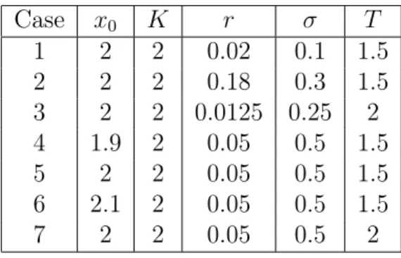
Table 2.1 reports the interest rate r, the volatility σ, the time to matu-rity T, the strike K and the initial asset price s0 for seven cases that will be

tested.

Table 2.1: Parameter values for seven test cases Case s0 K r σ T 1 2 2 0.02 0.1 1 2 2 2 0.18 0.3 1 3 2 2 0.0125 0.25 2 4 1.9 2 0.05 0.5 1 5 2 2 0.05 0.5 1 6 2.1 2 0.05 0.5 1 7 2 2 0.05 0.5 2

Table 2.2: Asian Call option prices when q=0 (parameters as in Table 2.1)

Case Order zero Order one FPP3 Linetsky Vecer MAE 3

1 0.0560415 0.0559965 0.05598604 0.05598604 0.055986 0.05598596 2 0.219607 0.218589 0.21838706 0.21838755 0.218388 0.21836866 3 0.172939 0.172738 0.17226694 0.17226874 0.172269 0.17226265 4 0.188417 0.194468 0.19316359 0.19317379 0.193174 0.19318824 5 0.248277 0.247714 0.24640562 0.24641569 0.246416 0.24638175 6 0.314568 0.307579 0.30620974 0.30622036 0.306220 0.30613888 7 0.355167 0.35361 0.35003972 0.35009522 0.350095 0.34990862

In the following table the same seven tests are repeated with a dividend rate equal to the interest rate. In this case the results of Linetsky and Vecer are not reported: the former because these tests were not considered in his paper; the latter because Vecer’s code cannot deal with that special case.

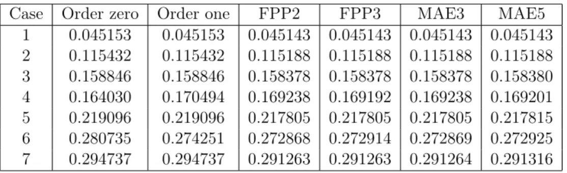
Table 2.3: Asian call option when q=r (parameters as in Table 2.1)

Case Order zero Order one FPP2 FPP3 MAE3 MAE5

1 0.045153 0.045153 0.045143 0.045143 0.045143 0.045143 2 0.115432 0.115432 0.115188 0.115188 0.115188 0.115188 3 0.158846 0.158846 0.158378 0.158378 0.158378 0.158380 4 0.164030 0.170494 0.169238 0.169192 0.169238 0.169201 5 0.219096 0.219096 0.217805 0.217805 0.217805 0.217815 6 0.280735 0.274251 0.272868 0.272914 0.272869 0.272925 7 0.294737 0.294737 0.291263 0.291263 0.291264 0.291316

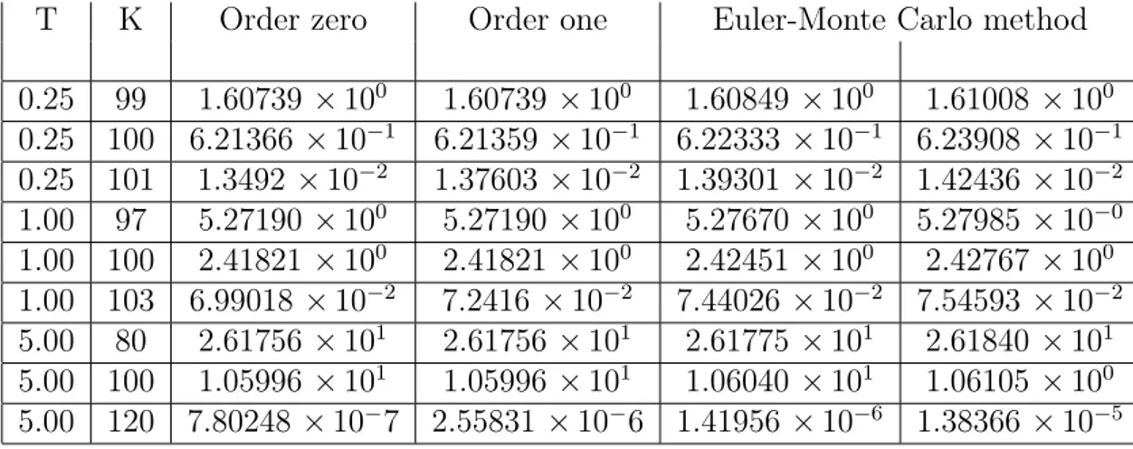
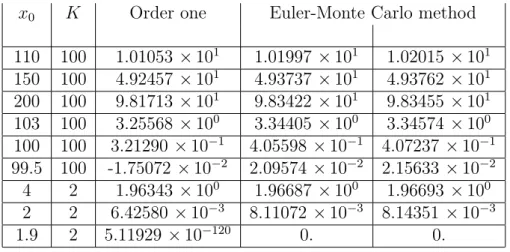
Next we tested our method with a low-volatility parameter σ = 0.01. Tables 2.4 shows the performances of the approximations against Monte Carlo 95% confidence intervals. These intervals are computed using 500000 Monte Carlo replication and an Euler discretization with 300 time-step for T = 0.25 and T = 1 and 1500 time-step for T = 5. In these experiments the initial asset level is s0 = 100, the interest rate is r = 0.05 and the dividend

yield is null q = 0. Table 2.5 shows the results of the methods FPP3, Vecer and MAE3 for the same parameters.

Table 2.4: Tests with low volatility: σ = 0.01 , s0 = 100 , r = 0.05 and q = 0

T K Order zero Order one Euler-Monte Carlo method

0.25 99 1.60739 × 100 1.60739× 100 1.60849× 100 1.61008 × 100 0.25 100 6.21366 × 10−1 6.21359× 10−1 6.22333× 10−1 6.23908× 10−1 0.25 101 1.3492× 10−2 1.37603× 10−2 1.39301× 10−2 1.42436× 10−2 1.00 97 5.27190 × 100 5.27190× 100 5.27670× 100 5.27985× 10−0 1.00 100 2.41821 × 100 _2.41821× 100 _2.42451× 100 _2.42767 × 100 1.00 103 6.99018 × 10−2 7.2416 × 10−2 7.44026× 10−2 7.54593× 10−2 5.00 80 2.61756 × 101 _{2.61756× 10}1 _{2.61775× 10}1 _{2.61840 × 10}1 5.00 100 1.05996 × 101 1.05996× 101 1.06040× 101 1.06105 × 100 5.00 120 7.80248 × 10−7 2.55831 × 10−6 1.41956× 10−6 1.38366× 10−5

Table 2.5: Tests with low volatility: σ = 0.01 , s0 = 100 , r = 0.05 and q = 0

T K FPP3 Vecer MAE3 0.25 99 1.60739× 100 _-4.18937 × 101 _1.60739 × 100 0.25 100 6.21359× 10−1 5.40466× 10−1 6.21359× 10−1 0.25 101 1.37618× 10−2 -3.96014 × 10−2 1.37615× 10−2 1.00 97 5.27190× 100 -9.73504 × 100 5.27190 × 100 1.00 100 2.41821× 100 _2.37512× 100 _2.41821 × 100 1.00 103 7.26910× 10−2 7.25478× 10−2 7.24337× 10−2 5.00 80 2.61756× 101 _{2.52779× 10}1 _{2.61756 × 10}1 5.00 100 1.05996× 101 1.05993× 101 1.05996 × 101 5.00 120 2.06699× 10−5 1.07085× 10−5 5.73317× 10−6

HARMONIC AVERAGE

3.1

Strategies tried

We consider a risky asset S following the equation in (1.15):

dSt = µ(t) Stdt + σ(t, St) StdWt (3.1)

where µ(t) = r(t)− q(t), is the difference between the risk-free rate and the dividend yield at time t, σ is the local volatility function and W is a standard real Brownian motion.

Now we consider as averaging price for the Asian option the state process given by the harmonic average:

Ht = ( ₁ t− t0 ∫ t t0 1 Su du )₋₁ (3.2)

For notational simplicity, we assume the starting time t0 is equal to zero.

We also assume that µ and σ are constants and we try to compute the price for an Asian option using the method seen in Chapter 1.

We have tried in different ways to arrive to this result, facing many obstacles and problems; eventually we got the results searched, even if in this case we obtained less accurate numeric results with respect to the arithmetic average case.

The first idea has been to describe the process (St, Ht) through a system of

stochastic equations similar to the one that we got in the arithmetic average case.

We can do this shifting the constant of normalization 1_t from the average to the payoff function and defining the following stochastic processes:

Xt = 1 St and Yt = 1 Ht (3.3) Then using the Ito formula (Theorem 1.1.1) we have:

dXt = d ( 1 St ) = − 1 S2 t dSt+ 1 2 2 St σ2S_t2dt = 1 St (σ2− µ) dt − 1 St σ dWt = (σ2− µ) Xtdt− σ XtdWt And dYt = d (∫ t 0 Xudu ) = Xtdt

Then the stochastic process is described by the following equations dXt = (σ2− µ) Xtdt− σ XtdWt

dYt = Xtdt

(3.4) The characteristic operator of this SDE is:

L = 1

2σ

2_x2_∂

xx+ (σ2− µ) x ∂x+ x ∂y+ ∂t (3.5)

This partial differential equation is then analogous to that we had in the case of the arithmetic average.

So we could get an approximation of its fundamental solution simply repeat-ing the same computations we have seen for the arithmetic average.

Despite that, we still couldn’t get an estimation for the price of the Asian option. Indeed we have seen that if Γ(t, s, a, T, S, A) is the fundamental so-lution for the characteristic operator of the SDE describing the process, and ϕ(S, A) is the payoff function, then the price is given by

v(t, T, s, a) = e−r (T −t) ∫

R2

Γ(t, s, a, T, S, A) ϕ(S, A) dS dA (3.6)

Now we recall that for the harmonic average we consider the following payoff function:

ϕ(S, A) = (HT − K)+ (3.7)

In this case we have:

ϕ(X, Y ) = ( T Y − K )+ (3.8)

So since ϕ has a non-integrable singularity in Y = 0 and we have seen in Chapters 1 and 2 that our approximation ΓN(t, x, y, T, X, Y ) of the

funda-mental solution for an operator like L is a Gaussian function in the variables (X, Y ), we have that ΓN(t, x, y, T, X, Y ) ϕ(X, Y ) diverge to infinity in Y = 0

and it is not integrable onR2_.

In conclusion we can’t use the processes Xt, Yt in (3.3) to compute the price

of an Harmonic averaged Asian option.

We have then tried to get an integrable payoff function without singular-ity using directly the dynamic of Ht instead of Yt. In this case however, we

haven’t be able to shift the normalization factor 1_t from the average to the

payoff function. Indeed if we consider only Ht =

( ∫t 0 1 Sudu )−1 , then the starting point H0 isn’t defined since

∫0 0

1

Sudu = 0.

On the contrary if we consider Ht =

( 1 t ∫t 0 1 Su du )₋₁

, then we can assume H0 = S0 since 1_t ∫t 0 1 Sudu→ S −1

0 for t→ 0 under suitable regularity

hypoth-esis.

Thus, starting again from the processes Xt, Yt in (3.3), we have computed

the dynamic of Ht: dHt = d ( 1 Yt ) = − 1 Y2 t dYt Where dYt = d ( 1 t ∫ t 0 Xudu ) = −1 t2 (∫ t 0 Xudu ) dt+1 t Xtdt = 1 t (Xtdt− Ytdt) Hence dHt = − 1 Y2 t 1 t (Xtdt− Ytdt) = 1 t ( Ht− Ht2Xt ) dt Then the operator related to the processes (Xt, Ht) is:

L = 1 2σ 2_x2_∂ xx+ (σ2− µ) x ∂x+ 1 t (h− h 2_{x) ∂} h+ ∂t (3.9)

Now we can proceed with our method computing as usual the Taylor series of σ2_x2 _{with respect to the point x}

0, and in addition, of h2 with respect to

the point h0. In this way the Taylor expansion of L at order zero is given by

L0 = 1 2σ 2_x2 0∂xx+ (σ2− µ) x ∂x+ 1 t h ∂h− 1 t h 2 0x ∂h+ ∂t (3.10)

Thus the approximation of order zero of the fundamental solution for L is

given by the fundamental solution of L0, which is the Kolmogorov operator

associated to the linear system d ( X_t0 H0 t ) = ( σ2− µ 0 −1 th 2 0 1t ) ( X_t0 H0 t ) dt + ( σ x0 0 ) dWt (3.11)

Then the fundamental solution for the operator L0 is given by the transition

density of the process (X0

t, Ht0).

In this case we haven’t been able to compute explicitly the transition density, though.

Indeed the function ϕ(t, T ) solution of the Cauchy problem (1.4) that is nec-essary to compute the expectation and the covariance matrix of the process (X_t0, H_t0) doesn’t have an analytic expression.

In conclusion we haven’t been able to get an analytic expression for the tran-sition density of the process.

An attempt to bypass this problem has been to consider the dynamic of Xt as in (3.3) and Ht =

(∫t

0 Xtdt

)₋₁

even if in this case H0 isn’t defined.

By the Ito formula, the process is described by the stochastic equation dXt = (σ2− µ) Xtdt− σ XtdWt

dHt = −XtHt2dt

(3.12) Then its characteristic operator is:

L = 1

2σ

2_x2_∂

xx+ (σ2− µ) x ∂x− h2x ∂h+ ∂t (3.13)

And so computing again the Taylor series of σ2_x2 _{with respect to the point}

x0, and of h2 with respect to the point h0 we get:

L0 =

1 2σ

2_x2

0∂xx+ (σ2− µ) x ∂x− h20x ∂h+ ∂t (3.14)

In this case we can explicitly compute the transition density of the linear system associated to L0 getting hence its fundamental solution Γ0. Thus we

can approximate the price computing explicitly the integral in (3.6) with Γ0

instead of Γ.

To solve the problem of the non-definition of H0 we have tried to assign to

it large values and we have seen the trend of the numeric results as H0 was

larger. This results didn’t converge to a sensible solution but remained ex-tremely low, even increasingly consistently the value of H0. In conclusion

they were totally disconnected from the ones we got using the Monte Carlo method.

Another attempt to compute the price of an Asian option with respect to the harmonic average has been to consider the following variable change

Xt := log ( St S0 ) Zt := log Yt = log 1 Ht = log1 t ∫ t 0 1 Su du (3.15)

Then by the Ito formula we have dXt = S0 St dSt+ 1 2 ( −S0 S2 t σ2S_t2dt ) = (µ−σ 2 2 ) S0dt + σ S0dWt dYt = d ( 1 t ∫ t 0 e−Xu S0 du ) = −1 t Ytdt + 1 t e−Xt S0 dt dZt = 1 Yt dt = −1 t dt + 1 t e Z0_e−Xt−Zt_dt

Where Z0 = log Y0 =− log S0; furthermore the payoff function is given by

ϕ(X, Z) = (e−Z − K)+

Which together a Gaussian function is integrable on R2

The characteristic operator of the dynamic is then:

L = σ 2_S2 0 2 ∂xx+ (µ− σ2 2 ) S0∂x− 1 t ∂z+ ez0−x−z t ∂z+ ∂t (3.16)

Now we can consider as L0 the following

L0 = σ2_S2 0 2 ∂xx+ (µ− σ2 2 ) S0∂x− 1 t ∂z+ ez0−x0−z0 t ∂z + ∂t (3.17)

But in this case, since there isn’t the term in x ∂z the covariance matrix of

the stochastic process related isn’t invertible and then it’s transition density haven’t got an analytic expression.

We can however approximate the term e−x−z with e−z0(1− x) by the Taylor

expansion of the exponential function; thus as L0 we can take:

L0 = σ2_S2 0 2 ∂xx+ (µ− σ2 2 ) S0∂x− 1 t ∂z+ 1 t (1− x) ∂z + ∂t (3.18)

Then we can compute explicitly its fundamental solution Γ0(t, x, z, T, X, Z)

and thus approximate the price computing the integral in (3.6) with Γ0

in-stead of Γ.

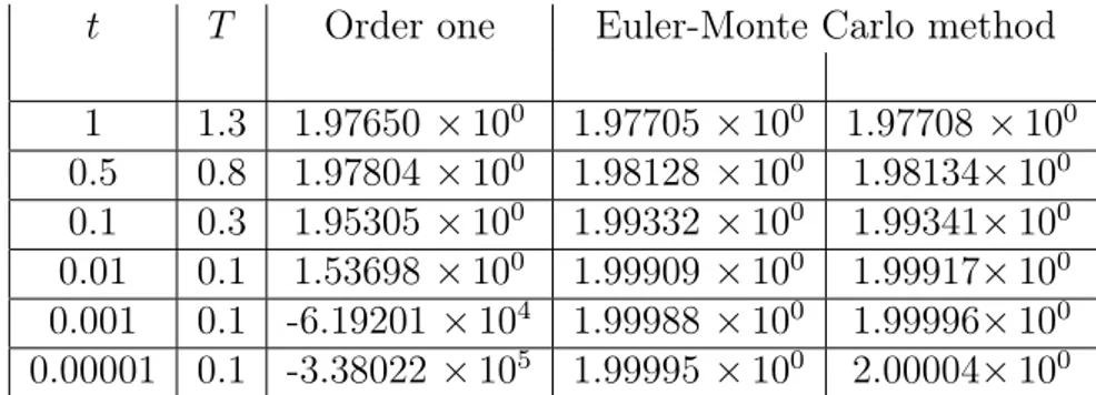
However the numeric results we have gotten haven’t been sensible. Indeed first of all we note that the equation L0 degenerate as t goes to zero, and so

does Γ0 and its integral with the payoff function.

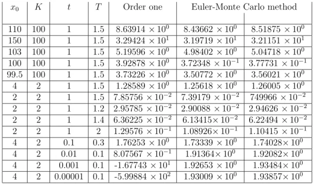
Furthermore even for t not close to zero our results aren’t comparable with the ones expected as shows the following table:

Table 3.1: Asian Call option prices when t = 1, T = 2, q = 0, K = 2

S0 2 2 2 1.9 2 2.1

r 0.02 0.18 0.0125 0.05 0.05 0.05

σ 0.1 0.3 0.25 0.5 0.5 0.5

Price: Our Method 2.047 2.451 2.020 2.073 2.093 2.114

Price: Monte Carlo Method 0.025 0.084 0.049 0.075 0.082 0.089

Certainly to obtain the operator L0 in (3.18) we have approximated an

exponential coefficient with a linear coefficient in x and this surely make us lose some accuracy but not enough to justify the results obtained in Table 3.1.

Thus there must be also another reason that explain our incorrect results. We have then understood that our attempt was wrong since we were using

a Gaussian function Γ0 to approximate a process Ht that had a Log-normal

distribution.

Therefore we have tried to change our approximation strategy to get sensible results.

Thus we have started again from:

dSt = µ Stdt + σ StdWt Ht = (∫ t 0 1 Su du )−1 _(3.19)

We have assumed for simplicity µ = 0 and considered: Xt := 1 St , Yt := e ∫t 0 Xudu (3.20)