ScienceDirect
Available online at www.sciencedirect.com
Procedia Structural Integrity 28 (2020) 53–60
2452-3216 © 2020 The Authors. Published by Elsevier B.V.
This is an open access article under the CC BY-NC-ND license (https://creativecommons.org/licenses/by-nc-nd/4.0) Peer-review under responsibility of the European Structural Integrity Society (ESIS) ExCo
10.1016/j.prostr.2020.10.007
10.1016/j.prostr.2020.10.007 2452-3216
© 2020 The Authors. Published by Elsevier B.V.
This is an open access article under the CC BY-NC-ND license (https://creativecommons.org/licenses/by-nc-nd/4.0) Peer-review under responsibility of the European Structural Integrity Society (ESIS) ExCo
ScienceDirect
Structural Integrity Procedia 00 (2019) 000–000
www.elsevier.com/locate/procedia
2452-3216 © 2020 The Authors. Published by ELSEVIER B.V.
This is an open access article under the CC BY-NC-ND license (https://creativecommons.org/licenses/by-nc-nd/4.0) Peer-review under responsibility of the European Structural Integrity Society (ESIS) ExCo
1st Virtual European Conference on Fracture
Modeling the cyclic plasticity behavior of 42CrMo4 steel with an
isotropic model calibrated on the whole shape of the evolution curve
Jelena Srnec Novak
a*, Marina Franulović
b, Denis Benasciutti
c, Francesco De Bona
aaPolytechnic Department of Engineering and Architecture (DPIA), University of Udine, via delle Scienze 206, 33100 Udine, Italy bFaculty of Engineering, University of Rijeka, Croatia
cDepartment of Engineering, University of Ferrara, via Saragat 1, 44122 Ferrara, Italy
Abstract
A durability analysis of a mechanical component generally requires accurate numerical simulations. For this purpose, the adopted cyclic plasticity material model should follow as closely as possible the material behavior observed during experimental testing. This work presents calibration of the isotropic material model for a 42CrMo4 steel, based on a series of cyclic fully-reversed tension-compression strain controlled tests performed at different strain amplitudes. Stress-strain cycles were recorded until end of each test with the goal to capture the isotropic stabilization effect of the material. As the isotropic model calibration gave poor results, if the exponential law proposed by Voce is adopted, an alternative Three parameters (TP) isotropic model is thus considered. The comparison with the experimental results show that the TP model fits significantly better the experimental results in almost all the considered cases. A possible justification of such improvement seems to be related to the fact that the equation governing the TP model contain a parameter that controls also the slope of the “S-shape curve” which describes the evolution of the material from initial to stabilized condition.
© 2020 The Authors. Published by ELSEVIER B.V.
This is an open access article under the CC BY-NC-ND license (https://creativecommons.org/licenses/by-nc-nd/4.0) Peer-review under responsibility of the European Structural Integrity Society (ESIS) ExCo
Keywords: low-alloy 42CrMo4 steel; material characterization; isotropic model;cyclic plasticity.
* Corresponding author. Tel.: +39-0432-558-297.
E-mail address: [email protected]
ScienceDirect
Structural Integrity Procedia 00 (2019) 000–000
www.elsevier.com/locate/procedia
2452-3216 © 2020 The Authors. Published by ELSEVIER B.V.
This is an open access article under the CC BY-NC-ND license (https://creativecommons.org/licenses/by-nc-nd/4.0) Peer-review under responsibility of the European Structural Integrity Society (ESIS) ExCo
1st Virtual European Conference on Fracture
Modeling the cyclic plasticity behavior of 42CrMo4 steel with an
isotropic model calibrated on the whole shape of the evolution curve
Jelena Srnec Novak
a*, Marina Franulović
b, Denis Benasciutti
c, Francesco De Bona
aaPolytechnic Department of Engineering and Architecture (DPIA), University of Udine, via delle Scienze 206, 33100 Udine, Italy bFaculty of Engineering, University of Rijeka, Croatia
cDepartment of Engineering, University of Ferrara, via Saragat 1, 44122 Ferrara, Italy
Abstract
A durability analysis of a mechanical component generally requires accurate numerical simulations. For this purpose, the adopted cyclic plasticity material model should follow as closely as possible the material behavior observed during experimental testing. This work presents calibration of the isotropic material model for a 42CrMo4 steel, based on a series of cyclic fully-reversed tension-compression strain controlled tests performed at different strain amplitudes. Stress-strain cycles were recorded until end of each test with the goal to capture the isotropic stabilization effect of the material. As the isotropic model calibration gave poor results, if the exponential law proposed by Voce is adopted, an alternative Three parameters (TP) isotropic model is thus considered. The comparison with the experimental results show that the TP model fits significantly better the experimental results in almost all the considered cases. A possible justification of such improvement seems to be related to the fact that the equation governing the TP model contain a parameter that controls also the slope of the “S-shape curve” which describes the evolution of the material from initial to stabilized condition.
© 2020 The Authors. Published by ELSEVIER B.V.
This is an open access article under the CC BY-NC-ND license (https://creativecommons.org/licenses/by-nc-nd/4.0) Peer-review under responsibility of the European Structural Integrity Society (ESIS) ExCo
Keywords: low-alloy 42CrMo4 steel; material characterization; isotropic model;cyclic plasticity.
* Corresponding author. Tel.: +39-0432-558-297.
1. Introduction
Constitutive modeling of cyclic plasticity has an important role to correctly predict the stress-strain evolution and consequently also to perform a durability estimation.
Over the last few decades, several plasticity theories have been developed with the aim to replicate more precisely a material behavior. Kinematic hardening can be modelled by adopting linear or nonlinear models (Prager, Armstrong and Frederick, Chaboche etc), while cyclic hardening/softening behavior can be captured with a nonlinear isotropic model (Voce), more details are given in Lemaitre and Chaboche (1990).
In a recent work presented by Basan et al. (2017), the material calibration has been presented for nonlinear kinematic (Chaboche) and isotropic (Voce) models based on experimental data for a 42CrMo4 low-alloy steel. A quite precise correlation has been obtained with the kinematic model, while in contrast, some discrepancy has been observed for the isotropic hardening behavior, modelled with a Voce model. As it will be shown, the exponential law of the Voce model hardly fitted the trend of experimental data, making the determination of the speed of stabilization fairly inaccurate. Similar results have been obtained also by other authors Koo and Kwon (2011), Goodall et al. (1980) for different types of steels.
With the aim of improving the accuracy of modeling a material cyclic evolution, a Three Parameter (TP) isotropic model (its governing equation is based on three parameter) have recently been developed by Srnec Novak et al. (2019). A first test, considering the cyclic behavior of a CuAg0.1 copper alloy at room temperature, has given quite promising results, confirming that the TP model is much closer to experiments than Voce model. In this work the TP isotropic model is adopted and tested considering the case of the 42CrMo4 steel.
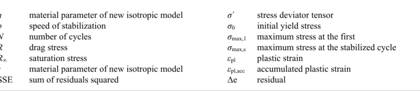
Nomenclature
a material parameter of new isotropic model σ´ stress deviator tensor
b speed of stabilization σ0 initial yield stress
N number of cycles σmax,1 maximum stress at the first
R drag stress σmax,s maximum stress at the stabilized cycle
R∞ saturation stress εpl plastic strain
s material parameter of new isotropic model εpl,acc accumulated plastic strain
SSE sum of residuals squared Δe residual
2. Experimental testing
The material considered in this work (42CrMo4 also named ISO 683/1 or AISI 4140) is a high-strength low alloy steel, frequently used for the manufacturing of mechanical components.
Following recommendations given by ASTM E606/E606M-12, specimens had a cylindrical unnotched geometry, with a smooth variation and a diameter from 10 to 7.7 mm, a total length of 105 mm and 27 mm gauge length. The steel was subjected to heat treatment processes (quenching and tempering) to provide a specific hardness. Specimens were heated to a temperature of 830 oC, quenched in oil bath and afterwards tempered for 1 h at temperatures of 630 oC, 480 oC and 300 oC to achieve respectively hardness of 296 HV, 420 HV and 546 HV. Experimental tests were
carried out at room temperature (20 oC) in strain-controlled mode on a servo-hydraulic Schenck Hydropuls test rig,
with a nominal force of 100 kN. The longitudinal elongation during test was recorded with HBM D4 model (ID101621900) extensometer (with a 25 mm gauge length). The tests applied a saw-tooth fully-reversed (Rε=-1) strain
waveform at a strain rate of 1.5 % s-1.
Three samples were tested for each hardness level and subjected to strain amplitudes in the range of 0.9÷1.8%. Decrease of 5% of the maximum stress σmax value in comparison to the values observed in the stabilized range was
taken as criterion for failure. More details about the experimental procedure are given in Basan et al. (2017).
Calibration procedure of material parameters for combined nonlinear kinematic (Chaboche) and nonlinear isotropic (Voce) models has been already described in Basan et al. (2017). Comparison between simulated and experimental stress-strain curves showed a good agreement in the case of kinematic model.
3. Theoretical background of cyclic plasticity
The yield criterion determines the stress level at which yielding occurs. In this work is considered the von Mises yield criterion defined in terms of the yield function f, Dunne and Petrinic (2005):
0 : 2 3 0 R f σ σ (1)
where σ՛ is the deviatoric stress tensor, R is the drag stress and σ0 is the initial yield stress (bold symbol indicate tensor). The variable R describes the expansion of the radius of the yield surface in the stress space. As can be noticed from Eq. (1), the evolution of the yield surface is described by scalars R and σ0. Variable R describes isotropic hardening or softening, while σ0 represents the size of the elastic area. The initial size of the yield surface is determined by using the criterion R=0.
3.1.Voce nonlinear isotropic model
Materials subjected to cyclic loading may exhibit cyclic hardening or softening behavior that can be captured numerically with an isotropic model. The isotropic model assumes that the center of the yield surface remains always at the origin and the surface enlarges or reduces homothetically in size as plastic strain εpl develops. In other words, according to Lemaitre and Chaboche (1990), evolution of the loading surface is governed only by one scalar variable, in this case, the accumulated plastic strain εpl,acc. The evolution equation of the commonly adopted nonlinear isotropic model (Voce) has the form:
1-exp-bεpl,acc
RR (2)
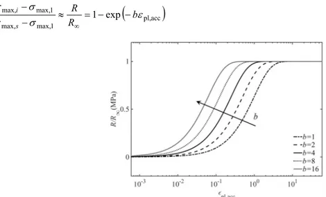
The governing equation is described by two parameters: b is the speed of stabilization, R∞ is the saturation stress that can be positive or negative representing either cyclic hardening (R∞ > 0) or softening (R∞ < 0), respectively. Evolution of the R is possible to express as the relative change of the maximum stress stress σmax,i in the Nth cycle with respect to the maximum stress in the first (σmax,1) and in the stabilized (σmax,s) cycle:
pl,acc
1 max, max, 1 max, max, 1 exp b R R s i (3)1. Introduction
Constitutive modeling of cyclic plasticity has an important role to correctly predict the stress-strain evolution and consequently also to perform a durability estimation.
Over the last few decades, several plasticity theories have been developed with the aim to replicate more precisely a material behavior. Kinematic hardening can be modelled by adopting linear or nonlinear models (Prager, Armstrong and Frederick, Chaboche etc), while cyclic hardening/softening behavior can be captured with a nonlinear isotropic model (Voce), more details are given in Lemaitre and Chaboche (1990).
In a recent work presented by Basan et al. (2017), the material calibration has been presented for nonlinear kinematic (Chaboche) and isotropic (Voce) models based on experimental data for a 42CrMo4 low-alloy steel. A quite precise correlation has been obtained with the kinematic model, while in contrast, some discrepancy has been observed for the isotropic hardening behavior, modelled with a Voce model. As it will be shown, the exponential law of the Voce model hardly fitted the trend of experimental data, making the determination of the speed of stabilization fairly inaccurate. Similar results have been obtained also by other authors Koo and Kwon (2011), Goodall et al. (1980) for different types of steels.
With the aim of improving the accuracy of modeling a material cyclic evolution, a Three Parameter (TP) isotropic model (its governing equation is based on three parameter) have recently been developed by Srnec Novak et al. (2019). A first test, considering the cyclic behavior of a CuAg0.1 copper alloy at room temperature, has given quite promising results, confirming that the TP model is much closer to experiments than Voce model. In this work the TP isotropic model is adopted and tested considering the case of the 42CrMo4 steel.
Nomenclature
a material parameter of new isotropic model σ´ stress deviator tensor
b speed of stabilization σ0 initial yield stress
N number of cycles σmax,1 maximum stress at the first
R drag stress σmax,s maximum stress at the stabilized cycle
R∞ saturation stress εpl plastic strain
s material parameter of new isotropic model εpl,acc accumulated plastic strain
SSE sum of residuals squared Δe residual
2. Experimental testing
The material considered in this work (42CrMo4 also named ISO 683/1 or AISI 4140) is a high-strength low alloy steel, frequently used for the manufacturing of mechanical components.
Following recommendations given by ASTM E606/E606M-12, specimens had a cylindrical unnotched geometry, with a smooth variation and a diameter from 10 to 7.7 mm, a total length of 105 mm and 27 mm gauge length. The steel was subjected to heat treatment processes (quenching and tempering) to provide a specific hardness. Specimens were heated to a temperature of 830 oC, quenched in oil bath and afterwards tempered for 1 h at temperatures of 630 oC, 480 oC and 300 oC to achieve respectively hardness of 296 HV, 420 HV and 546 HV. Experimental tests were
carried out at room temperature (20 oC) in strain-controlled mode on a servo-hydraulic Schenck Hydropuls test rig,
with a nominal force of 100 kN. The longitudinal elongation during test was recorded with HBM D4 model (ID101621900) extensometer (with a 25 mm gauge length). The tests applied a saw-tooth fully-reversed (Rε=-1) strain
waveform at a strain rate of 1.5 % s-1.
Three samples were tested for each hardness level and subjected to strain amplitudes in the range of 0.9÷1.8%. Decrease of 5% of the maximum stress σmax value in comparison to the values observed in the stabilized range was
taken as criterion for failure. More details about the experimental procedure are given in Basan et al. (2017).
Calibration procedure of material parameters for combined nonlinear kinematic (Chaboche) and nonlinear isotropic (Voce) models has been already described in Basan et al. (2017). Comparison between simulated and experimental stress-strain curves showed a good agreement in the case of kinematic model.
3. Theoretical background of cyclic plasticity
The yield criterion determines the stress level at which yielding occurs. In this work is considered the von Mises yield criterion defined in terms of the yield function f, Dunne and Petrinic (2005):
0 : 2 3 0 R f σ σ (1)
where σ՛ is the deviatoric stress tensor, R is the drag stress and σ0 is the initial yield stress (bold symbol indicate tensor). The variable R describes the expansion of the radius of the yield surface in the stress space. As can be noticed from Eq. (1), the evolution of the yield surface is described by scalars R and σ0. Variable R describes isotropic hardening or softening, while σ0 represents the size of the elastic area. The initial size of the yield surface is determined by using the criterion R=0.
3.1.Voce nonlinear isotropic model
Materials subjected to cyclic loading may exhibit cyclic hardening or softening behavior that can be captured numerically with an isotropic model. The isotropic model assumes that the center of the yield surface remains always at the origin and the surface enlarges or reduces homothetically in size as plastic strain εpl develops. In other words, according to Lemaitre and Chaboche (1990), evolution of the loading surface is governed only by one scalar variable, in this case, the accumulated plastic strain εpl,acc. The evolution equation of the commonly adopted nonlinear isotropic model (Voce) has the form:
1-exp-bεpl,acc
RR (2)
The governing equation is described by two parameters: b is the speed of stabilization, R∞ is the saturation stress that can be positive or negative representing either cyclic hardening (R∞ > 0) or softening (R∞ < 0), respectively. Evolution of the R is possible to express as the relative change of the maximum stress stress σmax,i in the Nth cycle with respect to the maximum stress in the first (σmax,1) and in the stabilized (σmax,s) cycle:
pl,acc
1 max, max, 1 max, max, 1 exp b R R s i (3)Plot of Eq. (3) for different values of b parameter shows that the curve shifts to the left by increasing the speed of stabilization (i.e. stabilized condition is reached at smaller vales of εpl,acc), while its “S-shape” remains essentially unaffected. In case of strain-controlled loading, the plastic strain range per cycle ∆εpl is approximately constant and the plastic strain accumulated after N cycles becomes equal to 2ΔεplN.
3.2.Three parameters (TP) nonlinear isotropic model
With the aim to improve fitting accuracy, Srnec Novak et al. (2019) proposed to modify Eq. (2), introducing a third parameter: s s a R R acc pl, acc pl, (4)
where a and s are material parameters that control the rate of cyclic hardening or softening. The proposed model has a physical basis, as it is able to capture the two limiting cases R = 0 for εpl,acc→0 and R = R∞ for εpl,acc→∞. The evolution of R can be described, similarly to the Voce model, by the relative change of the maximum stresses in each cycle: s s s i a R R acc pl, acc pl, 1 max, max, 1 max, max,
(5)Fitting of Eq. (5) to experimental data gives the values of a and s parameters; the estimation procedure to evaluate the saturation stress R∞ remains unchanged as it has the same physical meaning like in Eq. (2).
a) b)
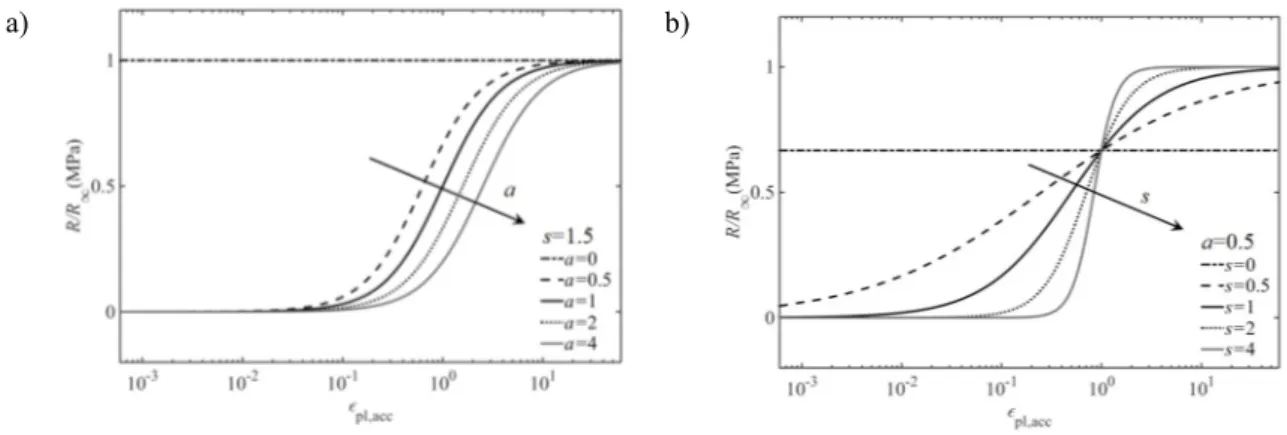
Fig. 2. The sensitivity of the proposed Eq. (5) to parameters (a) a and (b) s.
Sensitivity analysis of Eq. (5) is proposed in order to clarify the physical meaning of parameters a and s, see Fig. 2. Keeping constant s parameter and increasing values of a, the speed of stabilization diminishes and the curve shifts to the right. As can be observed in Fig. 2a), a bigger amount of the accumulated plastic strain is needed to reach the stabilized state. In contrast, see Fig. 2b), keeping constant a parameter and increasing values of s, “slope” of the increasing portion of the curve changes (i.e., higher values of s give a steeper average slope). Furthermore, it is possible to notice that limiting values exist for both parameters. For example, no cyclic hardening/softening would actually occur if a becomes either infinite (for which R = 0 for any s) or zero (for which R = R∞ from the first cycle). A similar behavior also occurs when s = 0, for which R = R∞/(a + 1). When s tends to infinite, R = 0 for εpl,acc < 1, R = R∞ for
εpl,acc > 1 and R = R∞/(a + 1) for εpl,acc = 1.
4. Results and Discussion
4.1. Calibration of the nonlinear isotropic models
Nonlinear isotropic parameters were estimated following procedure presented in Benasciutti et al. (2018). As 42CrMo4 steel never saturates completely, the maximum stress σmax over cycles continues to decreases and does not
approach any horizontal asymptote. Consequently, the number of cycle to reach stabilization was determined according to the conventional criterion given by Manson (1966) at half cycles to failure. The saturation stress R∞ was
determined considering the difference between the maximum stress in the first and in the stabilized cycle (R∞= σmax,1
- σmax,s) for each strain amplitude. Based on the obtained results (see Tab. 1), it is possible to conclude that material
exhibits softening behavior (R∞ < 0). The speed of stabilization b was estimated by fitting Eq. (3) to experimental data,
parameter a and s were similarly evaluated by using Eq. (5). Obtained results are reported in Tab. 1.
4.2. Isotropic models comparison
Figures 3 and 4 compare the Voce and the TP models with experimental data for different strain amplitudes and the three hardness levels (296 HV, 420 HV and 546 HV). In all exanimated cases, the Voce model follows a trend that deviates quite significantly from experimental data. The most relevant difference is observed for εa = 0.9% for all
three hardness levels. Such inconsistency is quite fully overcome by using the TP isotropic model, which fits better the experimental results in all the considered cases.
Results are compared by using residual Δe and sum of squared of residuals SSE that provide a “local” measure of fitting at each point and a “global” measure of fitting, respectively. The residual is defined as:
...n i y y for ,12 e exp,i model,i (6)
Symbol n denotes the number of experimental points used in calibration and subscripts model refer to the Voce or the TP model. To provide a single index value that quantifies the model accuracy for each strain amplitude, the sum of squares of residuals is calculated:
SSE 1 2 model, exp,
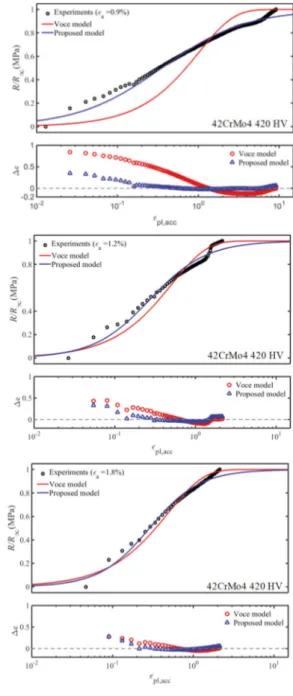
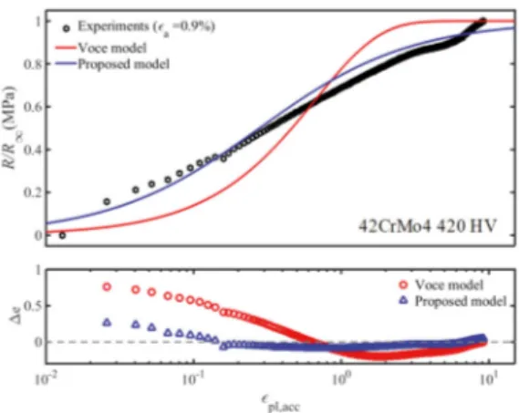
n i i i y y (7)Upper parts of the subplot of Figs. 3 and 4 depict fitting with Eqs. (3) and (5) considering Voce and the proposed model, respectively, while lower parts show residuals ∆e plotted on the vertical axis and the accumulated plastic strain (an independent variable) plotted on the horizontal axis. Figure 3 presents goodness of fitting for 0.9% strain amplitude of low-alloy 42CrMo4 steel and for two hardness levels (296 HV and 546 HV). On the other hand, Fig. 4 show calibration for different strain amplitudes (0.9%, 1.2% and 1.8%) of 42CrMo4 steel with 420 HV. In all exanimated cases, the residual Δe calculated with the proposed model is significantly smaller with respect to the Voce model especially at the first cycles.
As it can be noticed in Fig. 3a) and 3c), some experiments show a combination of cyclic softening and hardening behavior that basically cannot be captured with neither the Voce nor the TP model. In fact, as can be seen in Fig. 3b), both models show smaller residual Δe and SSE values if the last 30 experimental points (where the cyclic hardening is observed and which were taken into consideration in Fig 3a)), are neglected.
Plot of Eq. (3) for different values of b parameter shows that the curve shifts to the left by increasing the speed of stabilization (i.e. stabilized condition is reached at smaller vales of εpl,acc), while its “S-shape” remains essentially unaffected. In case of strain-controlled loading, the plastic strain range per cycle ∆εpl is approximately constant and the plastic strain accumulated after N cycles becomes equal to 2ΔεplN.
3.2.Three parameters (TP) nonlinear isotropic model
With the aim to improve fitting accuracy, Srnec Novak et al. (2019) proposed to modify Eq. (2), introducing a third parameter: s s a R R acc pl, acc pl, (4)
where a and s are material parameters that control the rate of cyclic hardening or softening. The proposed model has a physical basis, as it is able to capture the two limiting cases R = 0 for εpl,acc→0 and R = R∞ for εpl,acc→∞. The evolution of R can be described, similarly to the Voce model, by the relative change of the maximum stresses in each cycle: s s s i a R R acc pl, acc pl, 1 max, max, 1 max, max,
(5)Fitting of Eq. (5) to experimental data gives the values of a and s parameters; the estimation procedure to evaluate the saturation stress R∞ remains unchanged as it has the same physical meaning like in Eq. (2).
a) b)
Fig. 2. The sensitivity of the proposed Eq. (5) to parameters (a) a and (b) s.
Sensitivity analysis of Eq. (5) is proposed in order to clarify the physical meaning of parameters a and s, see Fig. 2. Keeping constant s parameter and increasing values of a, the speed of stabilization diminishes and the curve shifts to the right. As can be observed in Fig. 2a), a bigger amount of the accumulated plastic strain is needed to reach the stabilized state. In contrast, see Fig. 2b), keeping constant a parameter and increasing values of s, “slope” of the increasing portion of the curve changes (i.e., higher values of s give a steeper average slope). Furthermore, it is possible to notice that limiting values exist for both parameters. For example, no cyclic hardening/softening would actually occur if a becomes either infinite (for which R = 0 for any s) or zero (for which R = R∞ from the first cycle). A similar behavior also occurs when s = 0, for which R = R∞/(a + 1). When s tends to infinite, R = 0 for εpl,acc < 1, R = R∞ for
εpl,acc > 1 and R = R∞/(a + 1) for εpl,acc = 1.
4. Results and Discussion
4.1. Calibration of the nonlinear isotropic models
Nonlinear isotropic parameters were estimated following procedure presented in Benasciutti et al. (2018). As 42CrMo4 steel never saturates completely, the maximum stress σmax over cycles continues to decreases and does not
approach any horizontal asymptote. Consequently, the number of cycle to reach stabilization was determined according to the conventional criterion given by Manson (1966) at half cycles to failure. The saturation stress R∞ was
determined considering the difference between the maximum stress in the first and in the stabilized cycle (R∞= σmax,1
- σmax,s) for each strain amplitude. Based on the obtained results (see Tab. 1), it is possible to conclude that material
exhibits softening behavior (R∞ < 0). The speed of stabilization b was estimated by fitting Eq. (3) to experimental data,
parameter a and s were similarly evaluated by using Eq. (5). Obtained results are reported in Tab. 1.
4.2. Isotropic models comparison
Figures 3 and 4 compare the Voce and the TP models with experimental data for different strain amplitudes and the three hardness levels (296 HV, 420 HV and 546 HV). In all exanimated cases, the Voce model follows a trend that deviates quite significantly from experimental data. The most relevant difference is observed for εa = 0.9% for all
three hardness levels. Such inconsistency is quite fully overcome by using the TP isotropic model, which fits better the experimental results in all the considered cases.
Results are compared by using residual Δe and sum of squared of residuals SSE that provide a “local” measure of fitting at each point and a “global” measure of fitting, respectively. The residual is defined as:
...n i y y for ,12 e exp,i model,i (6)
Symbol n denotes the number of experimental points used in calibration and subscripts model refer to the Voce or the TP model. To provide a single index value that quantifies the model accuracy for each strain amplitude, the sum of squares of residuals is calculated:
SSE 1 2 model, exp,
n i i i y y (7)Upper parts of the subplot of Figs. 3 and 4 depict fitting with Eqs. (3) and (5) considering Voce and the proposed model, respectively, while lower parts show residuals ∆e plotted on the vertical axis and the accumulated plastic strain (an independent variable) plotted on the horizontal axis. Figure 3 presents goodness of fitting for 0.9% strain amplitude of low-alloy 42CrMo4 steel and for two hardness levels (296 HV and 546 HV). On the other hand, Fig. 4 show calibration for different strain amplitudes (0.9%, 1.2% and 1.8%) of 42CrMo4 steel with 420 HV. In all exanimated cases, the residual Δe calculated with the proposed model is significantly smaller with respect to the Voce model especially at the first cycles.
As it can be noticed in Fig. 3a) and 3c), some experiments show a combination of cyclic softening and hardening behavior that basically cannot be captured with neither the Voce nor the TP model. In fact, as can be seen in Fig. 3b), both models show smaller residual Δe and SSE values if the last 30 experimental points (where the cyclic hardening is observed and which were taken into consideration in Fig 3a)), are neglected.
a) a)
b) b)
c) c)
Fig. 3. Isotropic models for εa = 0.9% of 42CrMo4 steel with different
hardness levels ((a) 296 HV, (b) 296 HV without last 30 experimental points which show hardening, (c) 546 HV); Voce model (red line) and
proposed model (blue line). Residual ∆e is also reported.
Fig. 4. Isotropic model for different strain amplitudes of 42CrMo4 steel with 420 HV ((a) εa = 0.9%, (b) εa = 1.2% and
(c) εa = 1.8%); Voce model (red line) and proposed model
(blue line). Residual ∆e is also reported.
Only for the samples with a hardness of 296 HV, Voce model gives slightly smaller values of SSE with respect to the TP model. On the other hand, the TP model follows the experimental trend more accurately for the other two hardness levels and for all strain amplitudes. In fact, with respect to other cases available in literature, the considered material follows a quite smoother evolution trend and thus the slope of the “S-shaped” curve given by the exponential expression in Eq. (2) can hardly be adapted to fit such particular trend. On the contrary, the parameter s of the TP model permits the rate of transition from R(εpl,acc→0)=0 to R(εpl,acc→∞)=R∞ to be controlled.
Table 1. Isotropic parameters identified from experimental data for the Voce and proposed models. Goodness-of-fit examined in terms of sum of squares of residuals (SSE) for each model and strain amplitude.
Material hardness
Strain
Amplitude Material Parameters Error Index (SSE)
εa (%) R∞ (MPa) Voce Proposed Voce Proposed
b a s 296 HV 0.9 -94 1.158 0.388 2.054 0.348 0.518 1.2 -37 0.883 0.621 1.600 0.136 0.269 1.5 -104 1.312 0.327 1.608 0.018 0.082 Single values
R∞,ave1 ball1 aall1 sall1
1.169 1.597 -78 1.0861 0.4391 1.8091 420 HV 0.9 -328 0.986 0.419 0.832 4.749 0.347 1.2 -289 1.953 0.200 1.243 0.240 0.157 1.8 -265 2.027 0.176 1.394 0.077 0.048 Single values
R∞,ave1 ball1 aall1 sall1
6.853 1.932 -2941 1.4951 0.3371 0.8531 546 HV 0.9 -271 3.977 0.095 1.081 0.959 0.335 1.2 -323 3.516 0.089 1.347 0.082 0.080 1.5 -356 2.810 0.107 1.439 0.070 0.043 Single values
R∞,ave1 ball1 aall1 sall1 1.329 0.787
-3061 3.5101 0.0981 1.2151 1 parameters b
all, aall and sall are estimated from all experimental data merged together (whereas R∞,ave is the average over all
strain values).
Different values of R∞, b, a and s parameters characterize cycles with different strain amplitudes, see Tab. 1. This may represent a drawback, if commercial finite element codes have to be used, as they generally permit only one set of the isotropic parameters to be input. Furthermore, components subjected to cyclically loads usually undergo plastic deformations over different strain ranges. Therefore, adopted material parameters should be valid over a wider range of loading conditions. A possible compromise for solving this issue could be to take an average value R∞,ave and to identify a single value ball, aall and sall by fitting Eqs. (3) and (5), respectively, to all the experimental data gathered together (see Tab. 1). A comparison between the fitted curve calculated with the Voce model considering ball, the TP model with aall and sall parameters and the experimental data is presented in Fig. 5.
Fig. 5. Isotropic model for εa = 0.9% (42CrMo4 steel with 420 HV), calculated with ball, aall and sall
As expected, this “averaging” procedure makes the fitting slightly less accurate than those obtained by the parameters (b, a and s) specifically calibrated for each strain amplitude. Nevertheless, the TP model in most cases provides considerably better results in terms of SSE with respect to Voce model.
5. Conclusions
Materials subjected to cyclic loading may exhibit cyclic hardening or softening behavior whose evolution till stabilization can be described with an isotropic model. In most cases the nonlinear isotropic model proposed by Voce is able to fit well experimental data; this model is therefore widely adopted and implemented in several commercial FE codes. Nevertheless, in some cases materials shows a quite smooth evolution to stabilization. That is the case of the copper alloy analyzed in Srnec Novak et al. (2019) and of the low alloy steel considered in this work. In such cases the Voce model seems unable to fit well experiments; in fact, the exponential expression of the Voce model is characterized by only two parameters R∞ and b, that do not permit the slope of the “S-shaped” evolution curve to be
modified. To overcome this limitation, in the TP isotropic model a third parameter s is introduced, whose effect (see Figs. 3 and 4) permits also in the considered cases a good fitting to be achieved. The error analysis, confirm this statement, supporting the idea that, in some particular cases, the TP isotropic model could be a valid alternative to the Voce model.
References
ASTM E606/E606M – 12, Standard test method for strain-controlled fatigue testing 2012.
Basan, R., Franulović, M., Prebil, I., Kunc, R., 2017. Study on Ramberg-Osgood and Chaboche models for 42CrMo4 steel and some approximations, Journal of Constructional Steel Research 136, 65-74.
Benasciutti, D., Srnec Novak, J., Moro, L., De Bona, F., Stanojević, A., 2018. Experimental characterisation of a CuAg alloy for thermo‐mechanical applications. Part 1: Identifying parameters of non‐linear plasticity models, Fatigue & Fracture of Engineering Materials & Structures 41, 1364–1377.
Chaboche, J.L., 1986. Time-independent constitutive theories for cyclic plasticity. International Journal of Plasticity 2, 149–188.
Chaboche, J.L., 2008. A review of some plasticity and viscoplasticity constitutive theories. International Journal of Plasticity 24, 1642–1693.
Dunne, F. Petrinic, N., 2005. Introduction to computational plasticity; Oxford University Press: New York, NY, USA.
Goodall, I.W., Hales, R., Walters, D.J., 1980 On constitutive relations and failure criteria of an austenitic steel under cyclic loading at elevated temperature. In IUTAM Symp. Creep in Structures; Ponter, A.R.S., Hayhurst, D.R., Eds.; Springer–Verlag: Leicester, UK, pp. 103–127.
Lemaitre, J., Chaboche, J.L., 1990. Mechanics of solid materials, Cambridge University Press: Cambridge, UK. Koo, G.H., Kwon, J.H., 2011. Identification of inelastic material parameters for modified 9Cr-1Mo steel applicable to the plastic and viscoplastic constitutive equations, International Journal of Pressure Vessels and Piping 88. 26-33.
Manson, S.S., 1966. Thermal Stress and low-cycle fatigue, McGraw-Hill Book Company, Inc., New York. Srnec Novak, J., De Bona, F., Benasciutti, D., 2019. An isotropic model for cyclic plasticity calibrated on the whole shape of hardening/softening evolution curve, Metals 9, 1-13.