Computing in the Arts, a computational approach to Sculpture design.

UNIVERSITÀ DEGLI STUDI DI CASSINO E DEL LAZIO MERIDIONALE

Dottorato di Ricerca in

Metodi, modelli e tecnologie per l’ingegneria Ciclo XXXII

Computing in the Arts, a computational approach to Sculpture design.

Supervisors and co-supervisors PhD candidate

Prof. Maura Imbimbo Alfonso Oliva

2

INDEX

CHAPTER 1

THE HISTORICAL USE OF COMPUTATIONAL

METHODS

1.1 INTRODUCTION

1.2 BACKGORUND

1.3 STATE OF THE ART

1.4 THE RESEARCH INTENT

1.4.a Pre-design phase / feasibility study 1.4.b Schematic design (sd)

1.4.c Design development phase (dd) 1.4.d Construction documents (cd) 1.4.e Bidding

1.4.f Construction administration (ca)

1.5 THE NEW APPROACH TO DESIGN

CHAPTER 2

ALGORITHMS AS A MEANS TO DESIGN

2.1.a Background 2.1.b Research activity

2.1.c Introduction to concepts of optimization

2.2 ALGORITHMS OF OPTIMIZATION 2.2.a Choice criteria

2.2.b Description

3 2.2.b.ii Tabu Search 2.2.b.iii Genetic Algorithm 2.2.c Choice of the algorithm

2.2.c.i Applying GA to the Cantilever problem

CHAPTER 3

SOFTWARE SPECIFICATIONS

3.9.ii An algorithmic approach to documentation

CHAPTER 4

CASE STUDIES

4.1 FIRST CASE STUDY – ED CARPENTER 4.1.a Design and optimization workflow 4.1.a.i Loading conditions

4.1.a.ii Material 4.1.a.iii Connections 4.1.a.iv Observations 4.1.a.v Optimization steps

4

4.1.a.v.1 Improve performance through geometry manipulation

4.1.a.v.2 Improve performance through monitored material quantities

4.1.a.v.3 Improve performance through controlled stance width

4.1.a.vi Connection design 4.1.b Results

4.1.c Conclusions

4.2 SECOND CASE STUDY – ALYSON SHOTZ

CHAPTER 5

FROM RESEARCH TO PRODUCT

5.2 PRELIMINARY DESIGN

5.3 MATERIALS FOR 3D PRINTING

5.4 3D MODELING FOR FINITE ELEMENT ANALYSIS

5.5 FINITE ELEMENT ANALYSIS SET UP

5.6 SETTING UP THE OPTIMIZATION PROCESS

5.7 MULTI OBJECTIVE OPTIMIZATION 5.7.a Background

5.7.b Basics of MOO 5.7.c Pareto method

5 5.8 SETTING UP MOO OPTIMIZATION 5.9 FABRICATION

CHAPTER 6

FURTHER DEVELOPMENT AND POTENTIAL

APPLICATIONS

6 CHAPTER 1

THE HISTORICAL USE OF COMPUTATIONAL METHODS

1.1 Introduction

This research project aims on redefining design techniques and process for large scale sculptural works.

There has been a lot of innovation during the years in the Artistic field and particularly in the sculptural one. With the implementation during the last decade of advanced design techniques, like computational design (Fig.1), we find ourselves in an era where the concept of sculpture design can be completely redefined.

Fig. 1 Works from ICD Institute for Computational Design and Construction

Techniques like software development can now be paired with contemporary technologies such as algorithmic driven design, virtual reality, augmented reality and robotics, creating the strong basis for the innovation process in the Art field.

7

The proposed research project will explore some of the above mentioned techniques and combine those to prove how the combination of non-related fields can lead to a more efficient engineering design process.

1.2 BACKGROUND

Looking back at the history and evolution of sculpture design, there are few Artists that is worth mentioning for living a mark in the field of sculpture design.

To name a few and in temporary order, we find Willem de Kooning [1904], Kenneth Snelson [1927], Richard Serra [1938] and Alexander Calder [1898] amongst many other leading visionaries that in many different ways have helped shape and advance this field.

For the sake of the research, rather than focusing on their life, let’s focus directly on the typology of structures that they envisioned and built.

Starting in fact, with de Kooning highly abstracted figurative sculpture (Fig. 2) very reminiscent of his figurative paintings we move to the tensegrity sculptures of Kenneth Snelson delicate in appearance but very strong and depending only on the tension between rigid pipes and flexible cables (Fig. 3). From that, we look at the monumental corten steel large pieces (Fig. 4) from Richard Serra who became a pioneer of large-scale site-specific sculpture contrary to Alexander Calder’s medium scale kinetic sculptures (Fig. 5). Calder, known as the originator of the mobile, has in fact, pioneered a type of moving sculpture made with delicately balanced or suspended shapes that move in response to touch or air currents.

8

Fig. 2 Williem de Kooning

Fig. 3 Kenneth Snelson

9

Fig. 4 Alexander Calder

What is interesting though is what all these different minds have in common.

If we look more in depth at their bio, most of them have an artist background and that could certainly be a similarity but that’s not what made them unique. What made these sculptors pioneers in the field was the use of engineering techniques, whether it was mechanical, structural or electrical in some cases.

These names have strongly influenced my engineering and artistic side, helped them coexist, and have given me the inspiration to start this research project (Fig. 5).

10

Further motivation behind this work comes from the need of innovation to solve contemporary design problematics that are encountered daily in a typical design process for an Art piece. This point will be introduced and discussed in the next chapter.

1.3 State of the art

We, as an industry are advancing at a very slow pace. Who is there to blame? What do we have today that we didn’t have yesterday? and what else do we need? These are the most common questions that we hear in the EC (Engineering and Construction) industry. First problem being the nonintegrated design process and in particular the lack of conversation between Artist (Client) and Engineer (Consultant) from the early stage of the design. This, in fact, is the first obstacle to the implementation of new technologies to optimize the design and overall workflow.

Let’s explore that gap by looking at how the design workflow currently looks.

The current design process consists in a series of back and forth communications between the Artist and the Engineer that most of the times ends up being inefficient and counterproductive. What we just defined as “inefficiency” though, is nothing else that the use of two different languages, the Artistic language and the Engineering language. Establishing a good dialogue is key.

To further stress out the importance of the dialogue from the early stage of design, based on the experience accumulated over the years, it is safe to state, that even a sculpture conceptualized with the use of the latest software and technologies is, in most cases, not fully taking advantage from the technology itself because of the lack of

11

coordination amongst the different practices. The gap we are referring to though, is most of the times intangible.

This, is one of the problematic that this research project aims to address through the creation of what I define as a “sandbox” where both Engineers and Artist can meet and play together and speak the same language. That language in this case is called: “computational design”.

Before diving into the various opportunity that computational design offers, let’s look at other factors that have a big weight in the design process. Another more practical factor, is certainly costs. Costs are, in fact, often times the main driver and a brake on the implementation of new design process and/or technology.

That is only partially true though. It is in fact true only in the current design process where the above mentioned inefficiency of dialogue ends up consuming big part of the budget (up to 40% in some cases). The approach proposed in this research aims on bringing that percentage all the way down to 5% in some cases, to leave space for implementation of technology and advance the industry as a whole. Now that we understand that the main inefficiencies in the design process come down to something simple, yet complicated to get rid of, how do we tackle this factor that is so critical to guarantee a good outcome for each project?

Through example of successful case studies. The case studies below will show how the use of computational design techniques has brought back to life and to construction projects that were declared out of budget and dead.

To put it simple, we need to optimize. Computational Design techniques can help us do that, not strictly/only in the engineering process but rather in the design process a whole. An example of the

12

potential disruption that computational design can provide to the design process is presented by Ramboll UK and is shown in Fig. 6.

Fig. 6 Scheme of how Computational Design can disrupt the design process

Other side of the coin is that, as we aim on disrupting a design process that has been established for many years, we’ll have to face all the practical challenges that go with it.

Biggest challenge to face is to make the individuals collaborate and not challenge each other.

Computational Design and its related processes of optimization, in fact, is nowadays a practice and an actual form of art and for that reason needs to have enough space in the design process to be expressed. This often times does not convey with the idea or ego of the Artist that could take a more conventional or comfortable approach to his/her design.

Innovation comes in fact with a price. This last point, more aimed on the management of the design process is equally fundamental to achieve a successful outcome of the project.

13 1.4 The research intent

All in all the aim of the research is to find where computational processes fits and in which form within the design workflow to improve efficiency.

To understand and define that, we need to take a more in depth look at the current established design process.

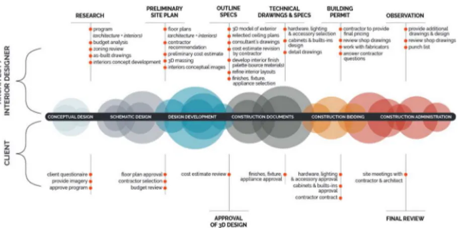
For a large scale sculpture the same design phases of an Architectural project apply. Here is a summary of all phases of design shown in Fig. 7.

There are six phases of design: Pre-design or feasibility study Schematic Design

Design Development Construction Documents Bidding

Construction Administration

14

1.4.a Pre-design phase / feasibility study

Pre-Design is a general term to describe the process prior to any form of actual design. This will include preliminary research on the site and the surrounding areas, scheduling and, if applies, any code restriction for the sculpture.

Essentially pre-design will be determining the information we need to begin design.

During this phase, the Artists also starts the so-called preliminary sketches, a mix of design and notes form the research. An example of a preliminary design sketch from Richard Serra is shown in Fig. 8.

Fig. 8 Richard Serra preliminary design sketch

1.4.b Schematic Design (sd)

The goal of schematic design is to start developing the shape and size of the piece with some basic integrated design thoughts. During this phase, overall plan views and 3D views are developed. Usually, most of the focus is centered on the final look of the piece

15

without many thoughts about the engineering of it. Figure 9 shows a schematic drawing from one of Alexander Calder mobile’s sculptures.

Fig. 9 Alexander Calder Schematic Design drawing

1.4.c Design Development (dd)

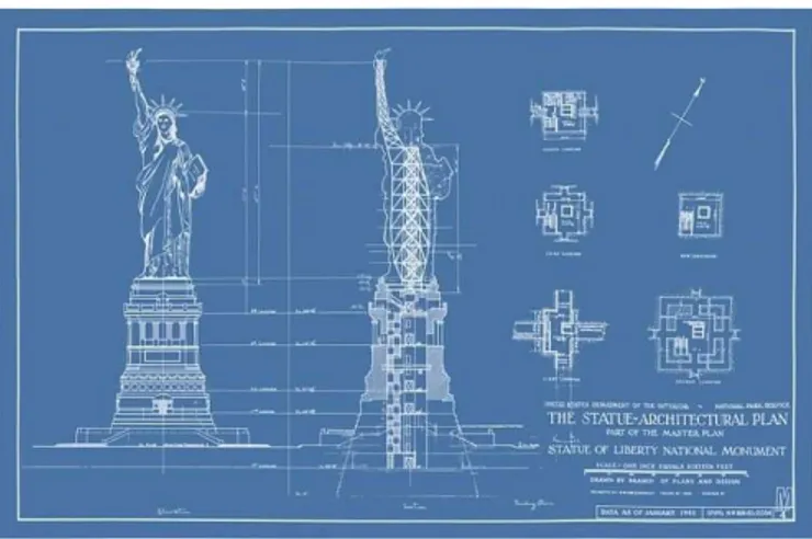
The aim of the dd phase is to transform and shape ideas into numbers.

In this stage, special attention is given to the structural system and the fabrication process. This helps explore different structural options and adapt ambitions to the project budget to make it buildable. This phase concludes when the design of the piece is locked in for the Artist and the Engineering and there is a clear understanding on the fabrication process. An example of the output of a dd phase is show in Fig. 10.

16

Fig. 10 Statue of Liberty blueprint

1.4.d Construction Documents (cd)

In the construction document phase all the technical design and engineering including structural engineering and detailing are finalized, and if needed, heating air conditioning and ventilation systems, plumbing, electrical, energy calculations, and all products and materials are selected and scheduled.

A drawing set including a filing set (required only for large pieces) for approval from the Department Of Buildings and a separate set of Construction Drawings is prepared. Fig. 11 shows an example of a construction drawing for a glass sculpture.

17 1.4.e Bidding

Bidding should be self-explanatory. This is the time to select a fabricator for the job to then proceed with construction. Multiple contractors submit bids on the job or the client can directly hire a contractor without getting competitive bids. In some cases, the engineer here will assist the client.

1.4.f Construction Administration (ca)

The Construction Administration is the final phase of the design process. While this phase is the longest, it does not usually comprise the majority of the work. On a typical project the engineer supervise construction. That means that the engineer will periodically visit the job site to check on progresses and ensure the contractor is following the plans.

This process has been historically adopted for the design of most sculptures as well as buildings.

1.5 The new approach to design

With time, and particularly in the last ten years, we have learned a lot from the above mentioned design process. To help this disruption, an interesting factor has helped re-shape and accelerate the design process, that factor is Computational Design.

Computational Design has in fact individually tapped into the different design phases and helped streamline the overall workflow as a whole.

Early adopter have certainly been fabricators. This means that the last phase of design (i.e. CA phase) it has actually been the first

18

phase of design to benefit from Computational Design processes and techniques.

Why is that? The answer is pretty straightforward: “Automation”. In fact, with the development of advanced design techniques more and more space has been given to automation tasks on the fabrication side. Two axis machine all the way up to 6 axis machine (aka robotic arms. See Fig. 12) have been implemented in the workflow to optimize the efficiency and precision of the fabrication process.

Fig. 12 Two robotic arms working on a sculptural piece

This is not news anymore though. Robotic arms, in fact, have been implemented for daily tasks by the industry.

The downstream seems to be covered in terms of implementation and even if there is more to do is well launched towards innovation. Fabrication is in fact considered as the downstream of the design process since is the step that precedes the delivery of the Art piece. With this research work we are proposing to enter from the other extreme of the design process: Schematic Design phase (SD phase).

19

As defined previously, SD is currently a phase where very minimal (if any) engineer is conducted.

This factor, has in my opinion and experience, historically lead many project over-budget. The reason behind this is the fact that the SD phase is all about developing the vision without any of the engineering thoughts that are instead introduced in the next phase. Computational Design processes can help us solve that and integrate engineering as early as the SD phase without compromising the Artistic vision.

Let’s then look at how we can make that happen. Specifically, we aim to understand how computational design can bridge the art and engineering field during SD and how that affects the subsequent phases of design.

To explain that, two case studies and one research project will be presented in the next chapters.

On a more practical level, Computational Design applied to the case studies presented in this research has allowed, through algorithm aided design to inform a large number of design intent in a relatively short amount of time. Without going in depth yet into the different algorithms that can be developed to optimize a design we can state, and later on prove with case studies, that the implementation of this technique in the design process is the key ingredient for a successful integrated design process.

20

CHAPTER 2

ALGORITHMS AS A MEANS TO DESGIN

2.1a Background

Technology is moving fast and is finally breaking into our industry. Technology ties directly into computational design, hence, engineering processes mainly given to their common base, algorithmic processes. This intersection allows us today to think about different workflows for the design of structures. To reiterate, although this thesis research aims on exploring different processes for sculpture design, this workflow can be applied to any kind of structure.

This chapter is an introduction on new workflows encompassing the same established engineering techniques we have used so far in our industry paired with optimization techniques to ensure the delivery of designs that preserve the Artist vision while being on budget.

2.1b Research activity

One other question we aim to answer in the following chapters is: Which are these established engineering techniques and how do they get combined with more contemporary workflows?

Established engineering techniques refer to the design of a structural element whether we are referring to a beam, a column or a façade panel. The way it gets combined with the current workflows is by attaching the variables contained in the design of the elements to

21

custom algorithms of optimization. The advantage behind that is that a large number of iterations can be performed in less time than a human could do with or without a conventional software.

2.1c Introduction to concepts of optimization

To introduce concepts of optimization explored, we’ll take as an example a cantilevered beam with a uniform distributed load [fig.13]:

Fig. 13 Cantilevered beam with distributed load

Our aim is to calculate the deflection in B:

where:

The aim is to optimize the design of the cantilever. The next question to be asked is, what do we want to optimize the beam for?

22 - Deflection (Comfort)

- Material quantities ($)

- Material usage (Weight of the structure)

The above mentioned factors could later on be combined to conduct a so called “multi-objective optimization”.

For this example we’ll focus on deflection only.

The first step is to pick the algorithm of optimization that we think is most useful for this task. This is in fact probably the most important part of the design process.

Every algorithm works in a different way and follows a different path. Some of them are affected by the initial configuration of the variables, some are affected by the previous iteration, some give a relative max or minimum, some give an absolute max or minimum.

2.2 Algorithms of optimization

The answer is not a straightforward one and most likely different people would pick different algorithms even when working on the same project. The key behind this kind of optimizations is in fact to be able to have a good understanding of the way the algorithm operates to be able to set up a solid algorithmic definition.

The three main algorithms we explored in this Research are listed below.

23 2.b Description

2.b.i Simulated annealing

This algorithm [Fig. 14] became very well-known after proving his benefits with outstanding performances when applied to optimization of a one-dimensional objective function [Fig. 15] but mostly when it was first applied to the “traveling sales man problem”, [Fig.16] problem where a salesman must visit some large number of cities while minimizing the total mileage traveled. If the salesman starts with a random itinerary, he can then pairwise trade the order of visits to cities, hoping to reduce the mileage with each exchange. The difficulty with this approach is that while it rapidly finds a local minimum, it cannot get from there to the global minimum. Simulated annealing improves this strategy through the introduction of two tricks. The first is the so-called "Metropolis algorithm" (Metropolis et al. 1953), in which some trades that do not lower the mileage are accepted when they serve to allow the solver to "explore" more of the possible space of solutions. Such "bad" trades are allowed using the criterion that:

where is the change of distance implied by the trade (negative for a "good" trade; positive for a "bad" trade), is a "synthetic temperature," and is a random number in the interval . is called a "cost function," and corresponds to the free energy in the case of annealing a metal (in which case the temperature parameter would actually be the , where is Boltzmann's Constant and is the physical temperature, in the Kelvin absolute temperature scale). If is large, many "bad" trades are accepted, and a large part of solution space is accessed. Objects to be traded are

24

generally chosen randomly, though more sophisticated techniques can be used.

The second trick is, again by analogy with annealing of a metal, to lower the "temperature." After making many trades and observing that the cost function declines only slowly, one lowers the temperature, and thus limits the size of allowed "bad" trades. After lowering the temperature several times to a low value, one may then "quench" the process by accepting only "good" trades in order to find the local minimum of the cost function. There are various "annealing schedules" for lowering the temperature, but the results are generally not very sensitive to the details.

There is another faster strategy called threshold acceptance (Dueck and Scheuer 1990). In this strategy, all good trades are accepted, as are any bad trades that raise the cost function by less than a fixed threshold. The threshold is then periodically lowered, just as the temperature is lowered in annealing. This eliminates exponentiation and random number generation in the Boltzmann criterion. As a result, this approach can be faster in computer simulations.

25

Fig. 16 Simulated Annealing optimization of a one-dimensional objective function

26 2.b.ii Tabu Search

Tabu Search [Fig. 16] is a Global Optimization algorithm and a Metaheuristic or Meta-strategy for controlling an embedded heuristic technique. Tabu Search is a parent for a large family of derivative approaches that introduce memory structures in Metaheuristics, such as Reactive Tabu Search and Parallel Tabu Search.

The objective for the Tabu Search algorithm is to constrain an embedded heuristic from returning to recently visited areas of the search space, referred to as cycling. The strategy of the approach is to maintain a short-term memory of the specific changes of recent moves within the search space and preventing future moves from undoing those changes. Additional intermediate-term memory structures may be introduced to bias moves toward promising areas of the search space, as well as longer-term memory structures that promote a general diversity in the search across the search space.

• Tabu search was designed to manage an embedded hill climbing heuristic, although may be adapted to manage any neighborhood exploration heuristic.

• Tabu search was designed for, and has predominately been applied to discrete domains such as combinatorial optimization problems.

• Candidates for neighboring moves can be generated deterministically for the entire neighborhood or the neighborhood can be stochastically sampled to a fixed size, trading off efficiency for accuracy.

• Intermediate-term memory structures can be introduced (complementing the short-term memory) to focus the search on

27

promising areas of the search space (intensification), called aspiration criteria.

• Long-term memory structures can be introduced (complementing the short-term memory) to encourage useful exploration of the broader search space, called diversification. Strategies may include generating solutions with rarely used components and biasing the generation away from the most commonly used solution components.

Fig. 16 Tabu flowchart

28 Taboo Search Java implementation

public State solve(State initialSolution) {

State bestState = initialSolution; State currentState = initialSolution;

int iterationCounter = 0;

//we make a predefined number of iterations

while(iterationCounter<Constants.NUM_ITERATIONS) {

//get all the available (reachable) states in the neighborhood

List candidateNeighbors = currentState.getNeighbors();

//get the tabu list

List solutionsTabu = tabuList.getTabuItems();

//get the best neighbor (lowest f(x) value) AND make sure it is not in the tabu list

State bestNeighborFound =

neighborSolutionHandler.getBestNeighbor(states, candidateNeighbors, solutionsTabu);

//we are looking for a minimum in this case if

(bestNeighborFound.getZ()<bestState.getZ()) {

bestState = bestNeighborFound; }

//we add it to the tabu list because we considered this item

tabuList.add(currentState);

//hop to the next state

currentState = bestNeighborFound;

iterationCounter++; }

//solution of the algorithm return bestState;

29

2.b.iii Genetic Algorithm

The genetic algorithm, (GA) is a method for solving both constrained and unconstrained optimization problems based on a natural selection process that mimics biological evolution. The algorithm repeatedly modifies a population of individual solutions.

In terms of analytical steps, there are two main operation in this algorithm, the selection and the crossover.

The selection process goes first, where two parent chromosomes gets selected from a population according to their fitness (the better fitness, the bigger chance to be selected) and then the crossover [fig. 18] of the parents takes place to form a new offspring (children).

Fig. 18 Example of crossover operation in Genetic Algorithm

2.c Choice of the algorithm

The three above mentioned algorithms have been implemented in the early stage of design for this case study. By monitoring speed and behaviors we were able to make a decision on which one to adopt for the whole optimization workflow.

The GA (Genetic Algorithm) was chosen for two main reasons: first one being speed. In fact, genetic algorithms seemed to be faster than

30

the other compared algorithms. Second, the fact that genetic algorithms is affected by the initial configuration of the “parents” (see explanation below) giving in a way more and more space to consider different solutions for the same design. Last but not least, genetic algorithms give in output a series of best performing solutions and not a unique one. This, applied to design translate in a large number of schemes with optimized performance that the artist can pick from.

All of this comes with a downside though. GA, in fact, can very easily produce results out of point of relative maximum or minimum. In other words, this kind of optimization does not guarantee the absolute optimal solution, but again, speed and the variety of exploration makes this a great candidate for these kind of optimizations.

2.c.i Applying GA to the Cantilever problem

The way we apply GA to the cantilever beam problem is the following. We assign as “Parents”, E and I with the aim of changing material properties and beam section to evaluate which are the best performing ones for the specific case.

By starting the process with an imaginary heavy member an imaginary weak material, the optimization process converges to a more reasonable result in few seconds.

I = 781250000 mm4

E = 200000 N/mm2

31

The way the algorithm converges to a solution is show in Fig. 19, 20 and 21 and discussed here:

Step 1 - Generate random population of n chromosomes (suitable solutions for the problem)

Step 2 - Evaluate the fitness f(x) of each chromosome x in the population

Step 3 - Create a new population by repeating following steps until the new population is complete

Step 4 - Select two parent chromosomes from a population according to their fitness (the better fitness, the bigger chance to be selected)

Step 5 - With a crossover probability cross over the parents to form new offspring (children). If no crossover was performed, offspring is the exact copy of parents.

Step 6 - With a mutation probability mutate new offspring at each locus (position in chromosome).

Step 7 - Place new offspring in the new population

Step 8 - Use new generated population for a further run of the algorithm

Step 9 - If the end condition is satisfied, stop, and return the best solution in current population

32

The aim of this simple exercise is, more than coming up with an optimized structure, to describe how GA convergences to a solution by starting with something that is far from an ideal desired output.

Fig. 19 GA Flowchart

33

Fig. 21 GA Representation

Fig. 22 and Fig. 22.a shows the GA solution for the problem of the traveling salesman previously presented for the simulated annealing.

34

Fig. 22.a Salesaman problem solved with GA

Once the basics of algorithmic techniques are established we can look into how these tools can be applied to the design of sculptures as in the case study below.

35 CHAPTER 3

SOFTWARE SPECIFICATIONS 3.1 Rhino

Rhinoceros [Fig. 23] (typically abbreviated Rhino, or Rhino3D) is a commercial 3D computer graphics and computer-aided design (CAD) application software. Rhinoceros geometry is based on the NURBS mathematical model, which focuses on producing mathematically precise representation of curves and freeform surfaces in computer graphics (as opposed to polygon mesh-based applications).

Fig. 23 Rhinoceros is widely used in processes of computational design.

Rhinoceros is primarily a free form surface modeler that utilizes the NURBS mathematical model. Rhinoceros’ open SDK (Software Development Kit) makes it modular and enables the user to develop custom commands.

Rhinoceros supports two scripting languages, Rhinoscript (based on VBScript) and Python (V5.0+ and Mac).

36

3.2 Grasshopper

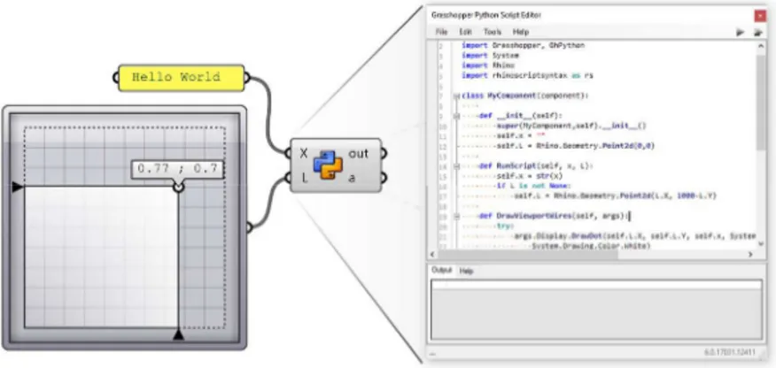
Grasshopper [Fig. 24] is a visual programming language and environment developed by David Rutten at Robert McNeel & Associates, that runs within the Rhinoceros 3D computer-aided design (CAD) application. Programs are created by dragging components onto a canvas. The outputs to these components are then connected to the inputs of subsequent components.

Fig 24 Grasshopper package for Rhino

Grasshopper is primarily used to build generative algorithms, such as for generative art. Many of Grasshopper’s components [Fig. 25] create 3D geometry. Programs may also contain other types of algorithms including numeric, textual, audio-visual and haptic applications.

Fig 25 Grasshopper components

Advanced uses of Grasshopper include parametric modelling for structural engineering [Fig. 26], parametric modelling for architecture and fabrication.

37

Fig 26 FEA solver for Grasshopper

The first version of Grasshopper was released in September 2007, and titled Explicit History. Grasshopper has become part of the standard Rhino toolset in Rhino 6.0 and later.

Grasshopper has been names as an endemic tool in the design world. The new Grasshopper environment provides an intuitive way to explore designs without having to learn to script and at the same time allows to write custom scripts within the application to push the boundaries of today’s work. This thesis will use default components in grasshopper as well as custom scripts [Fig. 27] developed for the purpose of the optimization processes.

38

3.3 Revit

Autodesk Revit [Fig.28] is a building information modelling software for architects, landscape architects, structural engineers, mechanical, electrical, and plumbing (MEP) engineers, designers and contractors. The original software was developed by Charles River Software, founded in 1997, renamed Revit Technology Corporation in 2000, and acquired by Autodesk in 2002. The software allows users to design a building and structure and its components in 3D, annotate the model with 2D drafting elements, and access building information from the building model's database.

Fig. 28 Revit environment

Revit is 4D building information modeling capable with tools to plan and track various stages in the building's lifecycle, from concept to construction and later maintenance and/or demolition. In this thesis project, Revit has been mentioned as the old standard for drawing production but not implemented in the workflow for documentation since this work relies on digital submission to fabricators. Revit has been implemented instead, together with

39

Virtual Reality for coordination on the location of one of the sculptures discussed later.

3.4 Dynamo

Dynamo is a visual programming tool that works with Revit. Dynamo extends the power of Revit by providing access to the Revit API (Application Programming Interface) in a more accessible manner. Rather than typing code, with Dynamo you create programs by manipulating graphic elements called “nodes” [Fig. 29]. It’s an approach to programming better suited for visually oriented types, like architects, designers, and engineers.

Fig 29 Dynamo nodes

In Dynamo, each node performs a specific task. Nodes have inputs and outputs. The outputs from one node are connected to inputs on another using “wires”. The program or “graph” [Fig 30] flows from node to node through the network of wires. The result is a graphic representation of the steps required to achieve the end design.

40

Fig 30 Dynamo Program

One of the strengths of visual programming and Dynamo, in particular, is ready access to a library of nodes [Fig 31]. Instead of having to remember the exact code you need to type to perform a certain task, in Dynamo you can simply browse the library to find the node you need.

Fig 31 Library of nodes

Likewise, a contributing factor to Dynamo’s success is its user community. In addition to providing help on its forum, Dynamo users can also create node libraries or “packages” [Fig. 32] and upload them to a central repository. This repository can be searched directly from inside of Dynamo. To install the package, simply click the download button and it will install directly into Dynamo.

41

Fig 32 Dynamo Packages

Dynamo has been utilized in this thesis work to prepare model coming into Revit for Virtual Reality.

3.5 Kangaroo

Kangaroo [Fig. 33] is a Live Physics engine for interactive simulation, form-finding, optimization and constraint solving.

It consists of a solver library and a set of Grasshopper components.

Installation instructions and a draft manual are included with the latest download.

42 3.6 Karamba

Karamba3D [Fig. 34] is an interactive, parametric finite element program. It lets you analyze the response of 3-dimensional beam and shell structures under arbitrary loads.

Fig. 34 Karamba for Grasshopper

3.7 Galapagos

Evolutionary solver plug-in for Grasshopper. Paired with parametric geometry allows for exploration of a large number of designs [Fig. 35].

43 3.8 CSI products

Computers and Structures, Inc. (CSI) is recognized globally as the pioneering leader in software tools for structural and earthquake engineering. SAP2000 [Fig. 36] is intended for use on civil structures such as dams, communication towers, stadiums, industrial plants and buildings and it has been used in this research to double check and confirm the results coming from the structural analysis conducted in Grasshopper with Karamba.

Fig 36 SAP 2000

3.9 Interoperability

The ability of graphical software to generate infinitely complex geometrical solutions using optimization techniques requires an equally concentrated effort to provide rational structural solutions. The growing experimentation with and implementation of Building Information Modeling (BIM), Parametric Modeling, and Structural Optimization requires software development and data management that are not a part of off-the-shelf software.

44

To better implement these techniques, part of the effort of this thesis work has been to bridge the gap between incompatible software to shorten the time between structural simulation (optimization) and structural reality (structural design).

The use of the techniques discussed in the following pages allowed for the rapid study of multiple SD level design options of the complex geometries shown in the case studies. Particular attention should be given to the flexibility and reaction time of these techniques in response to the Artist’s visions.

3.9.i The big picture

Here we describe the general approach to a design problem, software involved and workflow process.

In all below case studies we start from a Rhino model, received from the Artist. The Rhino model gets then discretized using Grasshopper, a process that involves building parametric definitions and developing algorithms that recreate the model accurately in a nonnative environment.

The discretization of the model aims to make the structure easier to analyze computationally by dividing it into simpler components. The simplification process is different for each kind of geometry. Frames are broken down into straight line segments, surfaces into smaller three- or four-sided surfaces, and volumes into six-sided shapes. Surfaces are then split based on the intersections of frames and walls, and non-planar surfaces are simplified by creating a mesh from which faces are extracted.

45

This is just the starting point of the design process. In the following sections, we will show how easily, through the use of a custom developed interoperability platform [Fig. 37], structural models and BIM models can be created in SAP2000/ETABS and Revit from a source Rhino model. The basic flow of this exchange is summarized by the diagram in Figure below.

Fig 37 Custom developed interoperability platform

Cuttlefish is composed of two separate components. The first component, developed in C#, reads data from an existing Grasshopper model and writes this data to an SQL database housed on a cloud server (Amazon Relational Database Service). The data that is read from the Grasshopper model is saved as a set of points, which represent the endpoints for frames and rigid links, as well as vertices for surfaces and volumes of the geometry. Once the user provides a project name, the data is written and stored in the cloud in the form of tables based on the type of geometry it originates from.

The MySQL database consists of a set of tables [Fig. 38] that store information from different sets of geometry: a table for frames, a table for volumes, etc. Each table is further subdivided into fields that store geometric information from the model, as well as unique structural analysis results (Figure below).

46

Fig 38 Example of MySQL database

The second component of the interoperability platform is a standalone docking application that serves as a container for software that does the translation work. This application, also developed in C#, reads the data stored in the cloud database and translates it to other software via their built-in API’s. The software carries information relative to geometry as well as structural analysis results from the CSI products.

The model can either be built from scratch or added onto an existing SAP2000 or ETABS model. This comes particularly in handy during multiple iterations conducted in parallel with the optimization process.

All of the work involved in the conversion is performed behind the scenes, yet all the data can be download in an excel spreadsheet at any time to design member sizes.

Building analysis models from an AWS server

The models generated with the interoperability platform for CSI SAP2000 and CSI ETABS will be used to perform structural

47

analysis for the sculptural pieces and also for their specific components and connection points.

Besides the difficulties inherent in building complex models into Finite Element Analysis (FEA) software with a high level of accuracy, the even greater challenge solved with this process is to be able to react quickly to changes made by the Artist. The parametric modeling environment, combined with the ad-hoc platform to transfer geometrical information and structural design, enabled a smooth design process.

The other advantage of using the interoperability platform was for the different sets design spreadsheets developed for the design of the structural members. Analysis results, stored in the cloud database, were output upon request through the Interoperability Platform. This workflow allowed to work on the same spreadsheet with set of analysis data coming from different design iterations parsed and organized in a consistent way. This process decreased the possibility of introducing errors and increased productivity (reading data from the cloud was, in this case, ten times faster than extracting results from an FEA model).

3.9.ii An algorithmic approach to documentation

In order to document the design, a Revit model was prepared and used to create drawings in combination with the digital 3D model deliverable for fabrication. The process of generating the Revit model was integrated into the workflow by creating a link between the architectural Rhino model, the structural analysis model, and Revit. This was done extending the interoperability platform to Dynamo for Revit.

48

In order to translate the geometry from the Rhino model into Revit, the point coordinate data, as well as the column connectivity and the surface data, were extracted from the Rhino model using the Cuttlefish component in Grasshopper and stored as tables in the cloud.

This geometric data was then used to generate a Revit model of the structural system. A custom node was developed in Dynamo to read the point coordinate data and element connectivity from the cloud in order to generate the sculpture in Revit. Once the structure had been analyzed in ETABS and element section sizes had been calculated, the next step in the workflow was to assign section properties to the elements in Revit. The model is now ready to be placed on sheets that will be part of the final deliverable.

49 CHAPTER 4

CASE STUDIES

4.1 First case study – Ed Carpenter

The first case study presented in this research is a sculpture by artist Ed Carpenter to be installed in a confidential building in Manhattan. Installation is estimated for the end of 2020.

The sculpture as schematically shown in fig.39 was conceptualized by the artist as a 45’ high piece composed by a large number of pipes supported by 10 columns.

Fig. 39 3D view of Artist vision for the sculptural piece

The sculpture initially designed by an Engineering firm in Manhattan was facing anticipated deflection under wind load of 3” (~8cm) as shown in fig. 40. Deflection in this case were not a problem, at least not yet. The sculpture in fact, was structurally sound and respected the deflection limits imposed by the code. The problem in this case was that the piece, given the current design, was over budget, and hence could not be built. The objective in this case was then to bring the project back in budget by optimizing the material usage while preserving the initial design and vision provided by the artist.

50

Fig. 40 3D view of Artist vision for the sculptural piece

4.1.a Design and optimization workflow 4.1.a.i Loading conditions

A first check of the existing loading assumption has been conducted. Fig 41 shows a comparison of the wind loads calculation (based on ASCE 7-10). In red there are the wind loads calculation from the original engineering design, in yellow there are the new wind loads based on my calculation. It is noticeable how the wind loads out of our calculations are 4 times higher than the original calculation. The reason for that is because of our assumption that the sculpture once installed on site will be covered because there will be construction around (4 buildings are being built on site). This, requested by the Artist, is to protect the piece until the surrounding works are completed.

51

Fig. 41 Wind loads comparison. Existing design VS new design

This assumption has consequences in the calculation of the deflection of course. By implementing the new wind load in the F.E. model developed throughout the software SAP2000, in fact, the deflection spike up to a 21” number as shown in Fig. 42.

52 4.1.a.ii Material

After checking the wind loads we moved into understanding the material utilized for the design. The engineering firm that was previously in charge of designing the piece had designed the sculpture to be in Steel. We wanted to make the sculpture lighter so we decided to explore Aluminum. This of course has its consequences. Aluminum has a strength that is 3 times less than steel. When inputting the mechanical properties of the Aluminum instead of the steel material of the SAP2000 model, we get what we already expected, a 60” deflection as shown in Fig. 43.

Fig. 43 Deflection increase due to change of material

4.1.a.iii Connections

The next logical step was to understand how the connection between the pipes and the columns worked. The previously engineered connection where a simple weld all over the sculpture. This process was working in advantage to strength but might have damaged the piece hence we studied a different solution. We decided to detail a saddle that would be shop welded on the column and upon which the pipe would be bolted on site [Fig. 44].

53

Fig. 44 Vertical pipe to saddle connection

This solution would definitely make the structure more flexible but at the same time produce a more elegant solution and prevent any damage to the Art piece. As expected, the deflection went up to 77” as shown in Fig. 45.

Fig. 45 Deflection increase due to pipe-saddle connection

4.1.a.iv Observations

At this point we not only had a structure that was over budget but also one that didn’t work structurally. This problem definitely opened an opportunity for optimization techniques.

4.1.a.v Optimization steps

We decided to tackle the problem in a 3-step optimization as summarized in Fig. 46 to 49.

54

First step, coordinated with the Artist, where we would shuffle the configuration of the pipes to guarantee maximum performance of the structure. The grasshopper definition is shown in Fig. 46

Fig 46 Shuffling pipes

Second step would aim on optimizing material usage rather than structural performance. This step would in fact assign different thickness to the pipes based on the stresses coming from the FEA. The grasshopper definition is shown in Fig. 47.

Fig 47 Thickness of pipes

The third and last step was a mix of material and structural optimization. Controlling the stance would in fact provide structural stability as well as minimize the material needed for the structure to be stable under wind loads. The grasshopper definition is shown in Fig. 48.

55

Fig 48 Stence of sculpture

Fig. 49 shows a visual summary of the three step optimization.

Fig. 49 Three step optimization

In order to do this, a custom defined Grasshopper definition was built and the plug in Galapagos and Karamba were used. Karamba is an FEA solver for grasshopper while Galapagos is an evolutionary solver that runs GA optimization. A localized screenshot of the grasshopper definition in Fig. 50 shows the input values for the optimization and the Galapagos interface running.

56

Fig. 50 Galapagos inputs and interface

The custom grasshopper definition allowed then to start the exploration for new solutions.

4.1.a.v.1 Improve performance through geometry manipulation The first step that consisted in reorganizing the pipes to achieve a stronger structural system lead to 6 main solutions allowing for a 40% reduction in deflection as shown in Fig. 51.

Fig. 51 Six best options out of the optimization process of Step1

To achieve this, a custom packing algorithm [Fig.52] has been developed in Grasshopper and then tied to FEA through Karamba and Galapagos to geometrically produce and calculate deflection for nearly 10,000 solutions amongst which the 6 best performing where then chosen and presented to the Artist.

57

Fig. 52 Custom packing algorithm developed for step 1

Form the above 6 option, the Artist picked option 5 as his preferred solution so we continued the study with the new geometry.

It is important to explain the nature and math behind the packing algorithm. Wolfram Math World gives a good explanation of that and it has been my source for the development of the work.

A circle packing [Fig. 52] is an arrangement of circles inside a given boundary such that no two overlap and some (or all) of them are mutually tangent. The generalization to spheres is called a sphere packing. Tessellations of regular polygons correspond to particular circle packings (Williams 1979, pp. 35-41). There is a well-developed theory of circle packing in the context of discrete conformal mapping (Stephenson).

58

The densest packing of circles in the plane is the hexagonal lattice of the bee's honeycomb, which has a packing density of:

Gauss proved that the hexagonal lattice is the densest plane lattice packing, and in 1940, L. Fejes Tóth proved that the hexagonal lattice is indeed the densest of all possible plane packings.

Surprisingly, the circular disk is not the least economical region for packing the plane [Fig. 53]. The "worst" packing shape is not known, but among centrally symmetric plane regions, the conjectured candidate is the so-called smoothed octagon.

Wells (1991) considers the maximum size possible for identical circles packed on the surface of a unit sphere.

Fig. 53 Circle disk region

Using discrete conformal mapping, the radii of the circles in the above packing inside a unit circle can be determined as roots of the polynomial equations:

59 with:

a ~ 0.266746 b ~ 0.321596 c ~ 0.223138

The following table gives the packing densities for the circle packings corresponding to the regular and semiregular plane tessellations (Williams 1979).

Solutions for the smallest diameter circles into which unit-diameter circles can be packed have been proved optimal for through 10 (Kravitz 1967). The best known results are summarized in the following table, and the first few cases are illustrated above (Friedman).

The best-known packings of circles into a circular shape are shown in Fig. 54 for the first few cases.

60

4.1.a.v.2 Improve performance through monitored material quantities

The second step [Fig. 55] conducted with the new geometry was solely looking at adding material where needed. This step compared 2 options, the one developed in this study that was parametrically exploring thousands of different configurations and picking the optimal material distribution and one that was the one adopted by the engineering firm that previously designed the sculpture. The step 2 in the optimization led to a reduction of the deflection of an additional 25%.

Fig. 55 Material distributed based on optimization VS more previous material distribution

4.1.a.v.3 Improve performance through controlled stance width The third and last step of the optimization focused instead on the stance. As previously mentioned, this was a mix of structural and quantities optimization as can be understood from Fig. 56. This step lead to an additional 25% in reduction.

61

Fig. 56 Example of difference stance configurations in step 3

4.1.a.vi Connection design

To ensure full design and constructability of the structural Art piece particular attention has been given to the pipe to pipe connection as shown in Fig. 57. This check has been conducted in the above workflow but not highlighted to keep the focus on the optimization workflow rather than the design of a detail.

Fig. 57 Pipe to pipe connection

4.1.b Results

Summing up all the contribution we come up to a 90% total reduction bringing the deflection down to 10” as shown in Fig. 58. The above study is a unitize study hence we now need to convert it

62

in real numbers that would give us an indication of how the sculpture is performing.

Fig. 58 Optimized solution performance

4.1.c Conclusions

Fig. 59 shows a comparison of the original structure VS the new optimized versions that achieved a 90% increment in performances thanks to the three-step optimization described in this summary. As can be understood by the visual, the vision of the Artist has been preserved while improving structural performance with custom optimization techniques.

63 4.2 Second case study – Alyson Shotz

The second case study is a sculpture by artist Alyson Shotz that is now installed in the new Kimmel NYU building in Manhattan.

The sculpture as shown in fig. 60 was conceptualized by the artist as a three story high piece composed by a large number of double curved ribs hanging from the ceiling. Each rib is composed by a sandwich of a layer of aluminum enclosed within two layers of acrylic.

This case study will be presented in a one chapter format with no subchapters to stress out the seamless continuity of the process.

Fig. 60 3D view of Artist vision for the sculptural piece

The sculpture initially designed by another Engineering firm in Manhattan was facing anticipated deflection under dead load at the bottom of the piece in the range of 96” (almost 245cm). This point raised the concern of many in the room especially the artist who all of the sudden was facing a totally different design from her initial concept idea. The objective was then to optimize the structural system to preserve the initial design and vision provided by the artist.

64

Given that no techniques are available out of the box for such a complex problem, I came up with an algorithm developed by myself. The algorithm, conceptualized in Rhino 3D (a cad software for designers) and Grasshopper 3D (a visual programming environment for Rhino) is based on the idea of merging the design provided by the artist with structural performance that resemble the concept behind the research, join engineering with artistic design.

The first part of the algorithm I put together in Grasshopper, allowed me to reconstruct a 3D model of the meshed structure of the desired configuration for the sculptural piece. The reason behind this is highlighted in the next paragraph.

Having a mesh, in fact, allowed me to link the 3D model with FEA and in order to achieve that I utilized Karamba (an FEA component for Grasshopper 3D) that was directly tight to the above mentioned algorithmic definition. By doing so I was able to confirm the 96” of deflection anticipated by the structural engineering firm that was on the job.

One other thing that I noticed during this process was that the sculpture was very easily thrown off balance when the location of the hanging cables changed. In fact, even by moving one of the three cables at the top by only few centimeters would give a huge increase in the value for the deflection.

That was then my next step and the starting point of the optimization process. I connected Galapagos (an evolutionary solver for Grasshopper that allows to run genetic algorithms) with my algorithmic definition and in particular, I defined the location of the cables as variables and the deflection calculated by Karamba based on the dead load of the sculpture as the value to be minimized.

65

This process lead to a relatively complex Grasshopper definition shown in Fig. 62

Fig 62 Grasshopper definition

After several attempts I collected a large number of data and picked the best performing cable configuration show later on in Fig. 63. This first step of the optimization allowed me to bring the value of the deflection down to 30”. Going down 66” in deflection was already a huge achievement but still too much.

For that reason, I moved into the next step of the optimization process, the camber. By in fact, back calculating the results given from the structural analysis, I was able to write a custom algorithm in C# language to camber the piece and analyze it to verify that the deflected shape of the cambered piece would coincide to the initial model provided by the artist.

The way the algorithm works is to retrieve results for the deflection at each single point of the mesh along the entire structure and apply the displacement with a negative sign to each correspondent point of the mesh.

66

Fig. 63 shows the initial geometry provided by artist in blue, the cambered shape in red and the final relaxed shape in lavender. It’s immediate to note that the relaxed shape is coincident with the desired shape.

Fig. 63 Comparison between desired, cambered and relaxed shape.

At this point, all the issue relatively to the structural performance are solved but one more issue comes up on the fabrication side.

The above mentioned algorithm used to camber the piece, in fact, makes the fabrication process impossible. The ribs of the cambered shape are, in fact, not perpendicular to each other anymore and that for that reason the piece, if cut by the CNC machine, cannot be assembled as the ribs wouldn’t fit together anymore.

This called for a third step in the optimization process and this time more for fabrication purposes. A third custom algorithm, in fact, was developed exclusively to deal with the perpendicularity of the ribs. The algorithm would get a single element of a mesh model, compute a small change in angle and compare this element against the other

67

in the desired perpendicular direction. The process would be performed on each single piece of the mesh and would stop when the 90 degrees angle configuration was reached.

The above mentioned algorithm has been developed discretizing the ribs into lines. This allowed to assume that each rib is in the form of: Ax+By+C=0

From this, the algorithm below can find and fix the perpendicular lines.

public class Perpendicular {

public static void main(String[] args) { Scanner in = new Scanner(System.in); int n=in.nextInt();

ArrayList<Line> list_of_lines=new ArrayList<Line>(); for(long i=0;i<n;i++){ long a=in.nextLong(); long b=in.nextLong(); long c=in.nextLong(); list_of_lines.add(new Line(a,b,c)); }

long p[]=new long[n]; Arrays.fill(p,0); for(int i=0;i<n;i++){ for(int j=1;j<n;j++){ if(list_of_lines.get(i).slope()*list_of_lines.get(j).slope ()== -1){

p[i]++;//num of perpendicular lines to i p[j]++;//num of perpendicular lines to j } } } } } class Line{

public long a,b,c;

public Line(long a,long b,long c){ this.a=a;

this.b=b; this.c=c; }

public double slope(){ return a/b;

68

Findings from this case studies can be summarized as follow. First, the integrated design process between artist and engineer resulted to be very efficient in terms of design performance and coordination. Moreover, the process included, as noted in the last paragraph, even the fabrication side that concludes the design cycle.

The algorithms developed for this specific case study can be applied to a large number of sculptural pieces. The other advantages in the use of this algorithmic technique is that each algorithms can be easily integrated to cover specific tasks in case needed for any other sculptural piece.

The sculpture is now installed in the NYU building on 31st street and 1st avenue in Manhattan, New York.

Fig 64 to 66 are some shots of the fabrication process showing the size of the modules produces that were later on assembled in place as seen in Fig 67 to 69

69

Fig 65 Fabricated module

70

Fig 67 Installed Sculpture

71

72 CHAPTER 5

FROM RESEARCH TO PRODUCT

During the last year of my PhD I wanted to merge all the above experiences under a product. The aim was to design an algorithmic driven sculpture that would be optimized for structural performance and completely conceptualized and driven by algorithms from conception (Schematic Design) to life (Fabrication).

5.1 The concept

Thanks to the advance in the computational field, sculptures today can embed different layers in their design. I will elaborate more on that:

- Artistic vision: As we all know Artists have a pretty specific vision for their pieces and most of the times little to no variations are permitted.

- Engineering thoughts: Structural design is the primordial need to any structure and sometimes does not walk hand in hand with the artistic vision.

- Computational thoughts: Computation is right in the middle of the Artistic vision and the Engineering thoughts. Computation helps to bridge that gap that goes from the 3D Artistic model to the current FEA software to the use of advanced algorithms to optimize the Artistic vision for structural performance without altering the Artistic vision.

The focus of this research is in that bridge. How do we pair conventional engineering tools with computational methods to preserve contemporary Artistic visions? The two case studies above have already partially answered this question and this chapter aims

73

on diving deep into it by exploring the full design process with a custom designed sculpture introduced in the next paragraphs.

The idea is to design a sculpture that would be easy to conceptualize but complex to analyze and fabricate with contemporary tools. The reason for that is because these are the future trends in the Art world. Artists are pushing the boundaries of complexity. They start with a concept that is easily realized in a 3D modeling environment but hides many Engineering and Fabrication challenges.

5.2 Preliminary design

The beginning of the research focused on two main basic Rhino commands:

Curves and polycurves;

Loft.

Following are the definitions provided by Mc Neel:

A Rhino curve is similar to a piece of wire. It can be straight or wiggled, and can be open or closed. A polycurve [Fig. 70] is several curve segments joined together end to end.

Rhino provides many tools for drawing curves. You can draw straight lines, polylines that consist of connected line segments, arcs, circles, polygons, ellipses, helices, and spirals.

You can also draw curves using curve control points and draw curves that pass through selected points.

Loft is a command in Rhino 3D that fits a surface through selected profile curves that define the surface shape.

74

Fig 70 Rhino polycurve

Fig 71 Rhino loft

Based on this approach I started by drawing 5 C-shaped [Fig 72] line segments spaced by 4cm.

75

Fig. 2D and 3D view of joined line segments to form a stack of c-shapes.

Later on, I referenced the c-shaped lines into grasshopper and subsequently divided them into segments of different lengths [fig. 73].

The points defined by this step are shown in the next figure and they will be driving the entire algorithmic definition and optimization process that will be described in the next paragraphs.

Fig 73 Subdivided C shape lines

The next step has been focused on creating curves [Fig 74] to give more movement to the backbone of the future sculpture.

The control points shown in the previous figure have then been fed into the Nurbs Curve command in Grasshopper to create 5 curves.

Fig 74 Lines to curves in Rhino

In order to make the constructing curves more dynamic a shift in the location of the points has been added [Fig 75]. Starting from two random function with the same slider as a driver, the X and Y