https://doi.org/10.1007/s40095-018-0265-9
ORIGINAL RESEARCH
Internal combustion engine heat release calculation using single‑zone
and CFD 3D numerical models
S. Mauro1 · R. Şener2 · M. Z. Gül2 · R. Lanzafame1 · M. Messina1 · S. Brusca3 Received: 30 October 2017 / Accepted: 12 February 2018 / Published online: 27 February 2018 © The Author(s) 2018. This article is an open access publication
Abstract
The present study deals with a comparative evaluation of a single-zone (SZ) thermodynamic model and a 3D computational fluid dynamics (CFD) model for heat release calculation in internal combustion engines. The first law, SZ, model is based on the first law of thermodynamics. This model is characterized by a very simplified modeling of the combustion phenomenon allowing for a great simplicity in the mathematical formulation and very low computational time. The CFD 3D models, instead, are able to solve the chemistry of the combustion process, the interaction between turbulence and flame propagation, the heat exchange with walls and the dissociation and re-association of chemical species. They provide a high spatial resolu-tion of the combusresolu-tion chamber as well. Nevertheless, the computaresolu-tion requirements of CFD models are enormously larger than the SZ techniques. However, the SZ model needs accurate experimental in-cylinder pressure data for initializing the heat release calculation. Therefore, the main objective of an SZ model is to evaluate the heat release, which is very difficult to measure in experiments, starting from the knowledge of the in-cylinder pressure data. Nevertheless, the great simplicity of the SZ numerical formulation has a margin of uncertainty which cannot be known a priori. The objective of this paper was, therefore, to evaluate the level of accuracy and reliability of the SZ model comparing the results with those obtained with a CFD 3D model. The CFD model was developed and validated using cooperative fuel research (CFR) engine experi-mental in-cylinder pressure data. The CFR engine was fueled with 2,2,4-trimethylpentane, at a rotational speed of 600 r/ min, an equivalence ratio equal to 1 and a volumetric compression ratio of 5.8. The analysis demonstrates that, considering the simplicity and speed of the SZ model, the heat release calculation is sufficiently accurate and thus can be used for a first investigation of the combustion process.
Keywords Internal combustion engines · Heat release · Single zone model · CFD combustion modeling
List of symbols
SOI Start of ignition TDC Top dead center IVC Intake valve closing Qhr Gross heat release k Specific heat ratio T Temperature
p Pressure V Volume
Qw Heat exchanged with wall Us Internal sensible energy W Work due to piston motion m Mass trapped
cv Specific heat at constant volume cp Specific heat at constant pressure Nu Nusselt number
Re Reynolds number
b Reynolds exponent for thermal exchange correlation
n Engine rotational speed C1, C2 Calibration constants
w Characteristic charge velocity up Average piston velocity pm Pressure of the motored cycle
p0, V0, T0 Reference pressure, temperature and volume
* S. Mauro
1 Department of Civil Engineering and Architecture,
University of Catania, Viale A. Doria, 6, 95125 Catania, Italy
2 Mechanical Engineering Department, Faculty
of Engineering, Marmara University, Kadikoy, 34722 Istanbul, Turkey
3 Department of Engineering, University of Messina, Contrada
ϕ Equivalence ratio
B Bore
y+ Non-dimensional distance from wall
mb Mass burned mu Mass unburned
kb, ku Burned and unburned specific heat ratios θ Crank angle
ρ Density
Introduction
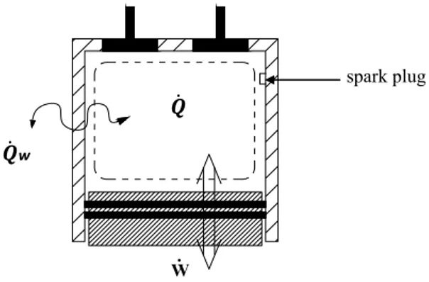
The complex task of improving internal combustion engines (ICEs), which have reached a higher degree of sophistica-tion, can be achieved with a combination of experiments and numerical models [1]. Essentially, two main distinct categories of numerical models have been developed for ICE studies. These are thermodynamic and fluid dynamic models. In the thermodynamic models, the conservation of mass and energy is used for evaluating the closed cylinder system using the first law of thermodynamics. In these mod-els, the thermodynamic system can be considered either as a single zone (SZ) or as a multi-zone. When the system is considered multi-zone, the first law of thermodynamics is applied to each of the zones while, in SZ models, the entire cylinder (Fig. 1) is the unique domain where the first law is solved. The mathematical equations, in general, form a set of ordinary differential equations with an independent variable, which is the time or the crank angle [2].
The heat transfer through the walls plays an important role in engine combustion, performance and emission char-acteristics [3, 4]. This is due to the fact that the wall temper-atures are considerably lower than the maximum tempera-ture of the burned gases inside the cylinder. For this reason, the heat transfer must be taken into account for an accurate modeling of the engine operative conditions [2].
Several thermodynamics models have been developed during the last few years, because of the great importance of
the heat release evaluation. The first simple models needed only in-cylinder pressure data but presented a great disadvan-tage: the assumption of a constant value for the polytrophic exponent [5]. Gatowski et al. developed a simple and quite accurate SZ model [6] which was further optimized for a charge with high swirl motion by Cheung and Heywood [7].
The thermodynamics model, developed in a previous work by the authors [10], is a SZ model which takes into account the variability of the specific heats [k = k(T)] and the heat exchange between gas and cylinder walls. In this way, both gross and net heat release can easily be calculated.
The fluid dynamic models, also known as computational fluid dynamics (CFD) models, are inherently unsteady, tridimensional models and are based on the conservation of mass, chemical species, momentum, and energy at any location within the engine cylinder domain. Thus, the CFD models solve the Navier–Stokes equations, and the gen-eral transport equations for each physical quantity. As is widely known, CFD models are based on numerical itera-tive techniques which lead to a set of equations filtered in time, named RANS equations, or in space, named LES equations. This is done in order to take into account the viscous stresses in a discretized computational domain that covers the whole cylinder volume [8]. Both time and spatial coordinates are considered independent variables, so a full spatial and temporal resolution of the properties of the gas inside the cylinder is possible [2]. In this way, the physics of the combustion process and, specifically, the flame propagation and its interaction with turbulence, is modeled. The heat release and the rate of heat release are, therefore, easily obtainable. Furthermore, the heat exchange with walls is taken into account using the real heat transfer coefficients.
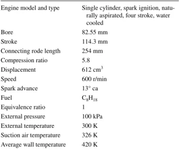
The cooperative fuel research (CFR) engine was used for the calibration and validation of both the thermodynamic and the CFD models. The CFR engine was developed by the Waukesha Motor Company, specifically for testing the knocking characteristics of fuels. This engine has an adjust-able compression ratio (CR), an adjustadjust-able ignition timing, and the capability to test fuels in sequence [8, 9]. The engine specifications and operating conditions used in this study are listed in Table 1.
The innovative idea presented in this paper is thus the development of a numerical methodology which is based on the joint use of SZ models and CFD models, in order to support ICE design and optimization and, specifically, the combustion modeling. Indeed, a direct experimental validation of the heat release calculation is very difficult to carry out and is usually missing in the scientific literature. Therefore, having a reliable CFD model of the combus-tion process would be a good reference for the evaluacombus-tion of the 0D model results. As the CFD models are certainly more physically accurate, the comparison between SZ and W.
̇
̇w
spark plug
Fig. 1 Control volume of the CFR engine combustion chamber in a single-zone model
CFD heat release calculation results may be very useful for a rapid evaluation of the predictive capabilities of a 0D model.
Numerical models
In this section, the main features of the numerical models are presented. Both the models were developed by the authors. While the SZ model was originally developed in a previous work and was adapted for this study [10], the CFD model
was specifically implemented in this work using the com-mercial solver ANSYS® Forte. Only the closed valves
condi-tion was considered for simulating the heat release; there-fore, the crank angle interval was between 214° and 500°. The fluid properties and all the relevant boundary conditions were exactly the same for both the models and are reported in Tables 1 and 2. These data were obtained during the CFR engine experimental tests.
Single‑zone model
The SZ model is a 0D model which has quite a good accu-racy of the physics of the phenomena and a great simplicity in the mathematical formulation [10]. The equation for the evaluation of the heat release rate is [6, 10, 11]:
In Eq. (1), both the dependence of k on temperature and the heat exchange with wall Qw are present.
The thermodynamic (pressure, temperature, composition, etc.) and transport (viscosity, conductivity, etc.) properties of the mixture are considered uniform in an SZ model. The thermodynamic state is calculated by applying the first law of thermodynamics. The application of the first law of ther-modynamics to the closed system in Fig. 1 requires an esti-mation of the heat loss between the combustion chamber and the walls. The relevant equation for the system in Fig. 1
reads: (1) dQhr= k(T) k(T) − 1pdV+ k(T) k(T) − 1Vdp+ dQw. (2) dUs= dQ + dW,
Table 1 CFR engine specifications and measured operating condi-tions (research method)
Engine model and type Single cylinder, spark ignition, natu-rally aspirated, four stroke, water cooled
Bore 82.55 mm
Stroke 114.3 mm
Connecting rode length 254 mm
Compression ratio 5.8 Displacement 612 cm3 Speed 600 r/min Spark advance 13° ca Fuel C8H18 Equivalence ratio 1
External pressure 100 kPa
External temperature 300 K Suction air temperature 326 K Average wall temperature 420 K
Table 2 Grid features, CFD settings and boundary conditions
Grid Grid 1 Grid 2 Grid 3
Number of cells ≈ 188,000 ≈ 500,000 ≈ 1,600,000
Global volume mesh size (mm) 2 1 0.5
Number of inflation layers on the walls 2 4 8
Calculation time (h) ≈ 3 ≈ 7 ≈ 24
Solver ANSYS Forte Unsteady-RANS
Time steps used 3 × 10⁻⁶ s
Solution algorithms SIMPLE, ALE method
Turbulence model RNG k–ε
Laminar flame speed model Gülder
Turbulent flame propagation model G-equation
Chemistry solver CHEMKIN Pro
Engine speed 600 rpm
Ambient pressure/temperature 100 kPa/300 K Air pressure/temperature at IVC 170 kPa/340 K
Average wall temperature 420 K
Initial turbulent kinetic energy 26,000 cm2/s2
where:
with the assumption that gas constant R does not change during the combustion process.
Substituting Eqs. (3)–(6) in the first law (2) and rearrang-ing the terms, it is possible to obtain the Eq. (1) for the heat release rate.
The heat exchange between the gas and cylinder walls is taken into account using the Woschni model [12]. In this model, the heat exchange coefficient is:
In Eq. (7) b is set to 0.8 (from the thermal exchange cor-relation: Nu = C Reb) and b is expressed in (m), p in (kPa),
v in (m/s) and T in (K). The expression for w is:
where p0, V0, and T0 are referred to the start of ignition
(SOI).
A polytrophic equation is used for the evaluation of pm [7, 10], where the exponent n is set to 1.3:
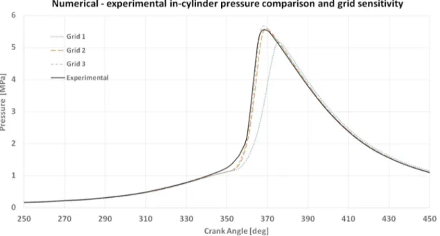
In the heat transfer model, C1 and C2 constants are not physical quantities and may differ from engine to engine. Changing these constants allows the model to be easily adjusted [7, 10]. Owing to these changes, these constants are calibrated with actual engine data. To comprise the heat release results, the SZ model is initialized using CFD cal-culated pressure data of the CFR engine. The CFD pressure data, in turn, were validated using experimental data of the CFR engine, as reported in Fig. 4. This was done in order to have the possibility to compare the heat release calcula-tions using identical pressure data thus allowing for a more meaningful comparison.
The specific heat ratio k has great influence on the heat release peak and on the shape of the heat release curve [10,
13, 14]. In this paper, a five-order logarithmic polynomial function (10) is used to provide the dependence of k on tem-perature [10]. (3) dW= −pdV, (4) dUs= mcv(T)dT, (5) dT= d(pV)∕mR, (6) R cv(T) = k(T) − 1 (7) hc= 3.26C1Bb−1pbT0.75−1.62bwb[W∕(m2K)]. (8) w= 2.28up+ 3.24 × 10⁻³C2 VT0 p0V0(p − pm), (9) pm= p0 ( V0 V )n . (10) k(T) = f{a0+ a1ln(T) + a2ln(T)2+ ⋯ + a5ln(T)5 } .
Since k depends on temperature and on charge composi-tion, and the mass fraction burned (MFB) is not dependent on the value chosen for the constant k [10], it is possible to write the function k(T) as:
where xb(T) is the MFB which can be evaluated from the
cumulative gross heat release with k = cost, starting from the Eq. (12):
where:
Further details about the SZ model can be found in [10]. Figure 2 shows a flow chart with the relevant steps for the SZ model calculation.
Computational fluid dynamics model
The unsteady CFD 3D model was developed using the com-mercial CFD software ANSYS® Forte. This software allows
for the simulation of combustion processes in ICEs. It does so using an efficient coupling of detailed chemical kinet-ics, liquid fuel spray and turbulent gas dynamics. ANSYS®
Forte can solve both the full unsteady RANS equations and the LES equations, thus providing accurate flame propaga-tion models with specific turbulent flame interacpropaga-tions. The following transport equation for the conservation of mass, momentum, energy and turbulence properties is solved:
where ϕ is the generic transported variable, Γϕ is the
convec-tion term, and Sϕ is the source term.
The conservation equation for the chemical species k is:
where ρ is the density, subscript k is the species index, K is the total number of species and u is the flow velocity vec-tor. The application of Fick’s law of diffusion results in a mixture-averaged turbulent diffusion coefficient DT. ̇𝜌k
c
and ̇
𝜌k
s
are source terms due to chemical reactions and spray evaporation, respectively.
The unsteady-RANS re-normalized group (RNG) k–ε model was used for turbulence modeling [15]. The RNG the-ory for turbulence calculations considers velocity dilatation
(11) k(T) = kb(T)xb(T) + [1 − xb(T)]ku(T), (12) xb(𝜗) = mb mu+ mb = Qgross|| |max Qgross(𝜗) , (13) Qgross(𝜗) = 𝜗 ∑ SOI ΔQhr. (14) 𝜕(𝜌𝜙) 𝜕t + ∇ ⋅ (𝜌̃u𝜙) = ∇ ⋅ (𝛤𝜙∇(𝜙)) + S𝜙, (15) 𝜕𝜌k 𝜕t + ∇ ⋅ (𝜌kũ) = ∇ [ ̄ 𝜌DT∇ ( 𝜌k ̄ 𝜌 )] + ̇𝜌kc+ ̇𝜌ks (k = 1, … , K),
in the ε-equation and spray-induced source terms for both k and ε equations: (16) 𝜕 ̄𝜌̃k 𝜕t + ∇( ̄𝜌̃ũk) = − 2 3𝜌̃k̄ ∇ ⋅ ̃u + ( ̄𝜎 − 𝛤 ) ∶ ∇̃u + ∇ ⋅ [(𝜇 + 𝜇 k) Prk ∇̃k ] − ̄𝜌 ̃𝜀+ ̇Ws,
In (16) and (17), cε are model constants, ̇Ws is the
nega-tive of the rate at which the turbulent eddies are doing work in dispersing the spray droplets and cs was sug-gested by Amsden based on the postulate of length scale conservation in spray/turbulence interactions. All these parameters are reported in [15].
The RNG k–ε model uses a standard wall function for the near-wall treatment. Therefore, the y+ was always kept
between 30 and 300 in the present work.
The use of advanced LES turbulence modeling was evaluated. However, the CFR engine was designed specifi-cally with very low turbulence levels inside the combus-tion chamber. The absence of significant swirl and tumble motions, due to the particular position of the intake and exhaust valves (Fig. 1), greatly simplifies the flow field inside the cylinder. Moreover, only the closed valves phase was modeled. For these reasons, the RNG k–ε model proved to be sufficiently accurate as widely demonstrated in the scientific literature [15, 16]. The numerical–experi-mental in-cylinder pressure data comparison presented in Fig. 4 further supports this assumption. An LES simula-tion would require a noticeable computasimula-tion time incre-ment without considerable advantages in the simulation accuracy.
The initial turbulent boundary conditions were esti-mated based on Heywood suggestions [17], according to the following formulas:
where kt is the initial turbulent kinetic energy, n is the engine rotational speed, Cμ is a model constant equal to 0.0845 [15],
ε is the dissipation rate and L is the turbulent length scale. The values are reported in Table 2.
The complex chemical reactions, which occur dur-ing the combustion process, are described by chemical kinetic mechanisms. These mechanisms define the reac-tion pathways and the associated reacreac-tion rates, thus leading to the change in species concentrations. The ANSYS Forte solver, coupled with the advanced chem-istry solver CHEMKIN-PRO, allows for the modeling of the chemical kinetics of all the K species related to the combustion process. Specifically, in this work, a (17) 𝜕 ̄𝜌 ̃𝜀 𝜕t + ∇( ̄𝜌̃u ̃𝜀) = − (2 3c𝜀1− c𝜀3 ) ̄ 𝜌 ̃𝜀∇ ⋅ ̃u + ∇ ⋅ [ (𝜈 + 𝜈k) Pr𝜀 ∇ ̃𝜀 ] + 𝜀̃ ̃k(c𝜀1( ̄𝜎 − 𝛤 ) ∶ ∇̃u − c𝜀2𝜌 ̃̄𝜀+ csẆ s). (18) kt= 1 2 [2 ⋅ stroke ⋅ n 60 ]2 , (19) 𝜀= C𝜇k 3∕2 t L, Ini alize with in-cylinder pressure data
Calculate Gross heat release with k constant
Calculate MFB with k constant
Evaluate k(T) from MFB and Gross heat release Interpolate real cp(T)
with VoLP
Calculate MFB with k(T)
Calculate Gross and Net heat release with k(T)
END
reduced mechanism chemistry set of 59 species (defined as Gasoline_1comp_59sp, which represents gasoline with the single-component iso-octane as the fuel surrogate) was used. The mechanism captures the pathways necessary for only the high temperature reactions and focuses only on capturing emissions from combustion. This mechanism was reduced from a larger kinetics mechanism consisting of ~ 4000 species, which has been thoroughly validated against fundamental experimental data for the operating conditions of interest in engines, under the “Model Fuels Consortium” [18]. The mechanism was originally reduced from this comprehensive “master” using the Reaction Workbench software. Iso-octane (C8H18) was used as a primary reference fuel in both the numerical and experi-mental analysis. The iso-octane properties were provided in the CFD code using the original CHEMKIN-PRO fuel database.
For the flame propagation modeling, the solver tracks the growth of the ignition kernel using the discrete particle igni-tion kernel flame model by Tan and Reitz [19]. Taking on the shape of a spherical kernel, the flame front position is marked by Lagrangian particles, and the flame surface den-sity is obtained from the denden-sity concentration of these par-ticles in each computational cell. The chemistry processes in the kernel-growth stage are treated in the same way as in the G-equation combustion model. A power-law correla-tion of laminar flame speed to pressure, temperature and equivalence ratio was chosen. This was the Gülder laminar flame speed formulation [20]. The Gülder reference formu-lation was developed and validated against numerous ICE experimental flame propagation data [21]. The equation for the laminar speed reads:
where the constants ω, η, ξ, σ are experimental data-fitting coefficients determined in [20, 21].
Once the laminar flame begins to develop within the cylinder domain near the spark plug, the flame–turbulence interaction is solved, based on the RNG k–ε transport equations. This results in a turbulent flame development. The turbulent flame speed can be controlled through a series of parameters. The local turbulent flame develop-ment is modeled by means of the G-equation, which pro-vides a strict correlation to the laminar flame speed which, in turn, is a chemical property of the gas mixture. The G-equation combustion model is based on the turbulent premixed combustion flamelet theory of Peters [22]. This theory addresses two regimes of practical interest. The first is corrugated flamelet regime where the entire reac-tive–diffusive flame structure is assumed to be embedded within eddies of the size of the Kolmogorov length scale η. The second is the thin reaction zone regime where the (20) S0L,ref= 𝜔𝜑𝜂
e−𝜉(𝜑−𝜎)2,
Kolmogorov eddies can penetrate into the chemically inert preheated zone of the reactive–diffusive flame structure, but cannot enter the inner layer where the chemical reac-tions occur. For application of the G-equation model to ICEs, this theory was further developed and validated by Tan and Reitz [19] and by Liang et al. [23, 24].
For the turbulent flame speed within the G-equation model, the following formula was used:
where IP is a progress variable, II and IF are the turbulence
integral length scale and the laminar flame thickness, b1,
b3 and a4 are generic for any turbulent flame and were cali-brated by Peters [22] by fitting experimental data.
The governing equations are discretized with respect to the spatial coordinates of the system on the computational grid, based on a control volume approach. In addition, in order to provide time-accurate solutions, the equa-tions are further discretized with respect to time, follow-ing the operator-splittfollow-ing method. To integrate the equa-tions in time, a temporal differencing of the equaequa-tions is performed. During time integrations, the solver employs three stages of solution for each time step. The time step-ping employs the operator-splitting method to separate the chemistry and spray source terms and the flow trans-port. The flow transport solution is based on the arbitrary-Lagrangian–Eulerian (ALE) method. Moreover, the solver uses a modified version of the SIMPLE implicit method, which is a two-step iterative procedure used to solve for the flow field variables. The SIMPLE method extrapolates the pressure, iteratively solves for velocities, then tempera-ture, and finally the pressure. Convection terms are instead solved using the quasi-second-order upwind method.
The chemistry solver employs an advanced operator-splitting method to solve the conservation of the species and energy conservation equations for time-accurate tran-sient simulations. This method splits the transport equa-tion into two sub-equaequa-tions and solves the sub-equaequa-tions with overlapping time steps.
The first step for the generation of the CFD model of the CFR engine was to reproduce the domain. In this case, the geometry was simply a cylinder with the dimensions reported in Table 1, which represented the combustion chamber, at that specific CR, when the piston was at the top dead center (TDC). Valves, intake and exhaust ducts, spark plug and crevices were neglected due to the fact that only the closed valves phase is essential for heat release calculations. However, this can only be done if the appro-priate boundary conditions are known. The boundary
(21) S0 T S0L = 1 + IP ⎧ ⎪ ⎨ ⎪ ⎩ −a4b 2 3 2b1 II IF+ ⎡ ⎢ ⎢ ⎣ � a4b2 3 2b1 II IF �2 + a4b23u �I I S0LIF ⎤ ⎥ ⎥ ⎦ 1∕2⎫ ⎪ ⎬ ⎪ ⎭ ,
conditions like pressure, temperature and composition at intake valve closing (IVC) were obtained from the CFR engine experiments and are reported in Table 2.
The spatial discretization is of utmost importance because of the necessity to find the best balance between accurate spatial resolution and reasonable calculation time. In light of this, a grid independence study was carried out. Structured hexahedral cells are generated by means of a dynamic mesh layering which is related to the piston motion within the crank angle interval (214°–500°). The layer dimension, and thus the minimum cell dimension, can be controlled by the user through the global volume mesh size control. Moreover, a prescribed number of infla-tion layers on the wall surfaces was used to improve the
solution of the thermal gradients. Three grid refinements, which were obtained by modifying the global volume mesh size and the number of inflation layers on the wall surfaces, were tested [25–27]. Details of the grids along with a summarization of the CFD settings are reported in Table 2.
The grid independent solution was evaluated by com-paring the in-cylinder pressure trends. When pressure trends did not significantly change with grid refinements, the solution was considered independent from the grid. This was obtained with the second refinement level (Grid 2), as reported in Fig. 3. In Fig. 2 a detail of the discre-tized computational domain with the piston at the TDC is shown.
The CFD solver allows for the specification of the spark plug characteristics. The spark starts 13 crank angle degrees before the TDC and the duration is 7°. The energy release rate for the specific spark plug was 50 J/s with an initial kernel radius of 0.5 mm.
The boundary condition for the head, the liner and the piston was a wall boundary condition with a prescribed wall motion for the piston surface which is determined by the rotational speed, the stroke, the connecting rod length and the crank angle interval. In doing so, the piston moves and generates the dynamic mesh layers at the same time (Fig. 3).
The initial premixed composition was provided using the specific composition calculation utility. The fuel was pure iso-octane with an equivalence ratio equal to 1. The calculation utility automatically defined the mass trapped and its composition from the knowledge of the fuel, the equivalence ratio and the boundary conditions at IVC.
Head - Wall, T = 420 K
Liner - Wall, T = 420 K
Piston head - dynamic wall, T = 420 K
Fig. 3 Detail of the discretized computational domain at TDC and boundary conditions
The simulations were carried out on an HP Z820 work-station with 24 available threads for parallel calculation and 128 Gb of RAM memory.
The convergence criteria were automatically checked by the ANSYS Forte solver in such a way as to ensure that all the residuals within each temporal step were below 10−6.
Results and comparisons
The main objective of this paper was to provide a numerical procedure in order to carry out a reliable evaluation of the heat release in ICE. The joint use of SZ 0D models and CFD 3D models leads to the possibility of an accurate calcula-tion of the heat release for numerous operative condicalcula-tions, without the need for further experimental data. The idea was to validate the CFD 3D model by comparing the numeri-cal–experimental in-cylinder pressure data. The calculated CFD pressure data were subsequently used for initializing the SZ model in order to have a precise and direct com-parison between the 0D and 3D heat release calculation. In doing so, it was possible to check 0D model accuracy and, eventually, understand how to modify and improve the SZ model. Moreover, the CFD model may provide different in-cylinder pressure data in such a way as to have the pos-sibility to run different operative conditions with both the models without the necessity of further experiments. Once the accuracy of the 0D model is checked, a fast and reliable heat release calculation can be obtained for a wide range of engine operative conditions.
The comparison between the CFD prediction of the in-cylinder pressure and the experimental measurements, pro-posed in Fig. 4, showed a good compatibility. Only slight differences are evident after the SOI, near 350 crank angle degrees and at the pressure peak. However, considering the general good accordance along the entire crank angle inter-val, the CFD model demonstrates quite a good predictive capability and can be considered experimentally validated for this specific condition.
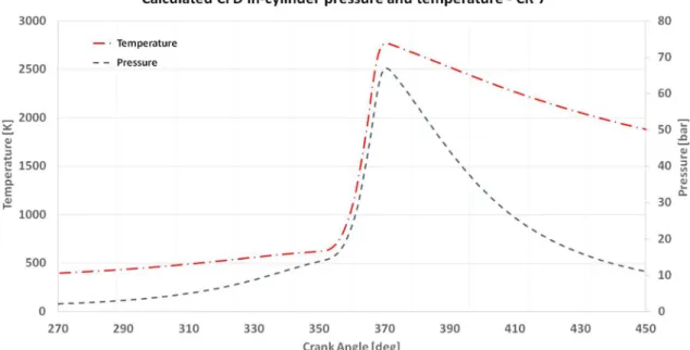
Two operating conditions of the CFR engine were ana-lyzed (CR = 5.8 and 7). The results for other CRs were quite similar and, therefore, are not presented. In Fig. 5, the calculated CFD in-cylinder pressure and temperature trend for the operating condition with CR = 7 is shown. These data were used for the initialization of the SZ model whose results are presented in the following figures.
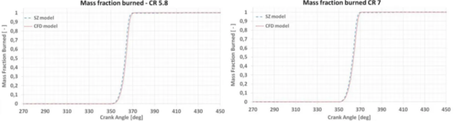
Specifically, in Fig. 6 the calculated MFB for the two dif-ferent compression ratios (CR = 5.8, 7), as a function of the crank angle position, is presented. The trend is very similar for both the operating condition and the differences between the numerical approaches are rather negligible. Considering the great simplicity and rapidness of the SZ model, the MFB appears to be well predicted.
In Fig. 7, the net heat release comparison is shown. The trend is quite similar for both the CRs. The SZ model shows an over-estimation which is probably due to the lack of the real chemical dissociation and re-association phenomena in the modeling. Indeed these phenomena are not taken into account in the SZ model. The chemistry solver within the CFD model, instead, is able to calculate the heat absorbed and released during the dissociation and re-association
reactions related to chemical species like NOx and CO.
Indeed, the differences between the models are drastically reduced after 400 crank angle degrees. This happened due to the fact that a part of the heat absorbed during the dis-sociation is given back with the chemical re-asdis-sociation [17]. Since the net heat release takes into account the heat exchange with walls, the discrepancies evidenced at 450 CA are certainly due to the differences in the heat transfer
modeling between the models. This comparison will thus be very helpful in the improvement of the Woschni heat exchange model.
The above is confirmed by the heat release rate compari-son proposed in Fig. 8 and the gross heat release comparison shown in Fig. 9. Indeed, in Fig. 8, both models predict a sim-ilar ROHR trend in the initial combustion phase. The ROHR peak, instead, is higher in the CFD results but the subsequent
Fig. 6 Calculated mass fraction burned for CR 5.8 (left) and CR 7 (right)
Fig. 7 Calculated cumulative net heat release for CR 5.8 (left) and CR 7 (right)
decrease is faster. This denotes a different dynamic of the combustion prediction between the numerical models. More-over, after 375 crank angle degrees the CFD model predicts a small amount of heat release due to chemical dissociation and re-association phenomena (Figs. 10, 11). However, the global trend of the ROHR is quite similar for both the mod-els and the operating conditions, therefore, demonstrating an acceptable reliability of the SZ model.
In Fig. 9, the gross heat release calculation results are presented. Nevertheless, in the CFD model the flame is quenched at near 370 crank angle degrees (Fig. 6), then a small amount of heat is gradually released from 370 to 440 crank angle degrees. In fact, the gross heat release is actu-ally the heat release due to a combination of all the chemi-cal reactions (combustion, dissociation, re-association). Therefore, the different trend between the models in Fig. 9
Fig. 9 Calculated gross heat release for CR 5.8 (left) and CR 7 (right)
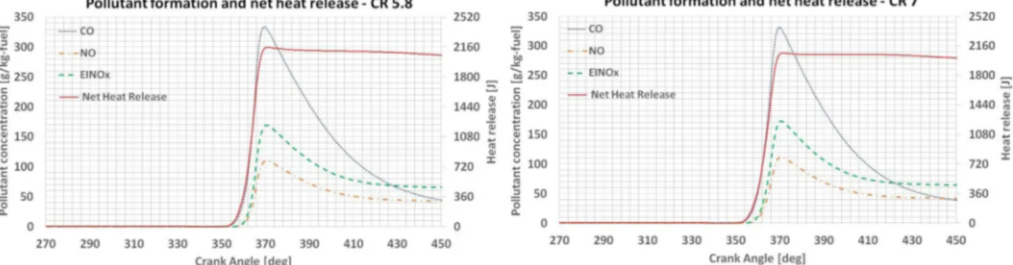
Fig. 10 Pollutant formation and net heat release for CR 5.8 (left) and CR 7 (right)
is ascribable to chemical reactions which initially absorb a part of the heat generated by the combustion (dissociation) and then gradually release heat during the expansion phase (re-association) [17]. However, the final value of the cumula-tive gross heat release is very compatible for both the operat-ing conditions. Thus, the SZ model lacks the capability of predicting the real combustion dynamics but demonstrates accuracy in the evaluation of the cumulative heat, released during the combustion. No strong differences are evident between the two analyzed operating conditions.
The presented results demonstrate that the use of powerful CFD models would be very helpful for the validation of SZ models. Moreover, from the comparison of the calculated heat release, one can easily identify the areas in which the SZ model may be improved in order to reduce errors. Further possibilities are to calibrate the SZ model for the simulation of the use of different fuels, water injections or other combustion control strategies. This will be done in future works. The CFD model allows for an engine virtualization which may limit the experi-ments, thus providing an accurate and reliable reference for the SZ model heat release calculation of any other engine at any operative condition. Moreover, the CFD model is able to pro-vide details about the in-cylinder flow field, the chemical reac-tions, the pollutant formation, the flame development which may be of utmost importance for 0D model improvements and, in general, for ICE analysis and optimization. Clearly, the pro-posed numerical procedure must be implemented, verified and calibrated case by case, based on the engine type. The present work would, therefore, propose an innovative idea for a better evaluation of the heat release calculation in ICEs.
In conclusion, in Fig. 10 the calculated CFD pollutant for-mation along with the net heat release is shown. The details provided by the CFD analysis support the previous hypothesis that the chemical dissociation and re-association phenomena influence the gross heat release evidenced in Fig. 9. Indeed, as expected, during the expansion phase, the chemical re-association releases a small amount of heat which has been absorbed during the initial combustion phase. This explains the differences highlighted in Figs. 7, 8, and 9. During the first stage of the combustion, the pollutant formation absorbs heat which is gradually restored in the expansion phase. Since the SZ model does not take into account the dynamics of the chemical reactions, in the first combustion phase the SZ model overestimates the heat release while in the expansion phase the error is balanced by the heat restored due to the chemi-cal re-association. In Fig. 11, the NO2 formation is compared
with the in-cylinder temperature trend, calculated through the ANSYS Forte simulation. Also, in this case, a strong relation between temperature and pollutant formation is clearly evident.
Some of the numerous possibilities offered by the com-bustion virtualization, obtained with the proposed CFD model, are presented in the figures above. The opportunity to have a powerful tool, which might not only be a fundamental
reference for the validation and optimization of the SZ model [for example the calibration of the constants of the Eq. (8)], can be inferred. The joint use of both SZ and CFD 3D models would be an important numerical methodology for the study and the optimization of ICEs, therefore, reduc-ing the expensive heat release experimental analysis.
Conclusions
In the present study, two different numerical models, an SZ model and a CFD model, were implemented for the simu-lation of the closed part of the cycle of a CFR engine in order to obtain an accurate heat release evaluation. The CFD model was validated using the in-cylinder pressure data for the CFR engine, fueled with pure iso-octane, with a volu-metric CR of 5.8 in the research method test condition. The CFD in-cylinder pressure data were subsequently used for the initialization of the SZ model in order to obtain a perfect comparison of the heat release calculation capabilities.
Despite the strong mathematical simplicity and the extreme rapidness of the SZ model, the comparison between 0D and CFD 3D heat release calculations demonstrates that the SZ model is sufficiently accurate and reliable. The CFD model is obviously more physically accurate and allows for a reliable prediction of the chemical reactions and, thus, for the heat absorbed and released because of them. However, the calculation time for the CFD model is higher by several orders of magnitude.
In the specific case of the CFR engine, the main differ-ences between the models were found to be due to the lack of the chemical kinetics in the SZ model and partially to the wall heat exchange model of Woschni which probably necessitates further calibrations case by case.
The proposed model comparison shows the perspectives of the joint use of both 0D and CFD 3D model for ICE combustion investigations. On the one hand, the CFD model will be a powerful reference for the improvements of the SZ model, thanks to the possibility of detecting the areas where the 0D model is not as accurate. Moreover, the CFD model may provide numerous in-cylinder pressure data by vary-ing the volumetric CR, the equivalence ratio, the rotational speed and so on. This may allow the SZ model to virtually run any kind of engine operative condition without the need for further experimental data. In this way, although the heat release calculations are already obtained with the CFD anal-ysis, the possibility to have accurate references may allow the SZ model to be calibrated and improved in a wide range of conditions. On the other hand, having a reliable numeri-cal strategy, with the joint use of 0D and CFD 3D models, will be a very powerful tool for the investigation and the optimization of the combustion phase in ICEs.
Therefore, the present study intends to provide a 0D–3D numerical procedure for the analysis of the heat release in ICEs which will have to be further refined and validated on other types of engines with different operating conditions. Both models must be implemented, refined, calibrated and validated specifically on the engine characteristics.
In light of this current information, future works in this field will regard the improvement of the SZ model for a wide range of engine operating conditions. Moreover, fur-ther studies will be made on the implementation of specific modifications, in the 0D model, for the simulation of com-bustion control strategies like water injections or for the use of alternative fuels.
Compliance with ethical standards
Conflict of interests On behalf of all the authors, the corresponding author states that there is no conflict of interest.
Open Access This article is distributed under the terms of the Crea-tive Commons Attribution 4.0 International License (http://creat iveco mmons .org/licen ses/by/4.0/), which permits unrestricted use, distribu-tion, and reproduction in any medium, provided you give appropriate credit to the original author(s) and the source, provide a link to the Creative Commons license, and indicate if changes were made.
References
1. Lakshminarayanan, P.A., Aghav, Y.V.: Modeling Diesel Combus-tion. Springer (2010). https ://doi.org/10.1007/978-90-481-3885-2. ISBN 978-90-481-3885-2
2. Medina, A., Curto-Risso, P.L., Hernández, A.C., Guzmán-Var-gas, L., Angulo-Brown, F., Sen, A.K.: Quasi-dimensional Simu-lation of Spark Ignition Engines. Springer (2014). https ://doi. org/10.1007/978-1-4471-5289-7. ISBN 978-1-4471-5289-7 3. Heywood, J.B.: Internal Combustion Engines Fundamentals.
McGraw-Hill (1988). ISBN 0-07-100499-8
4. Neshat, E., Saray, R.: Effect of different heat transfer models on HCCI engine simulation. Energy Convers. Manag. 88, 1–14 (2014). https ://doi.org/10.1016/j.encon man.2014.07.075
5. Rassweiler, G., Withrow, L.: Motion Pictures of Engine Flames Cor-related with Pressure Cards. SAE Technical Paper 380139 (1938). https ://doi.org/10.4271/38013 9
6. Gatowski, J., Balles, E., Chun, K., Nelson, F. et al.: Heat Release Analysis of Engine Pressure Data. SAE Technical Paper 841359 (1984). https ://doi.org/10.4271/84135 9
7. Cheung, H., Heywood, J.B.: Evaluation of a One-Zone Burn-Rate Analysis Procedure Using Production SI Engine Pressure Data. SAE Technical Paper 932749 (1993). https ://doi.org/10.4271/93274 9 8. Brock, C., Stanley, D.L.: The cooperative fuels research engine:
applications for education. J. Aviat. Technol. Eng. (2012). https :// doi.org/10.5703/12882 84314 865
9. Broekaert, S., De Cuyper, T., De Paepe, M., Verhelst, S.: Evalu-ation of empirical heat transfer models for HCCI combustion in a CFR engine. Appl. Energy 205, 1141–1150 (2017). https ://doi. org/10.1016/j.apene rgy.2017.08.100
10. Lanzafame, R., Messina, M.: ICE gross heat release strongly influ-enced by specific heat ratio values. Int. J. Automot. Technol. 4(3), 125–133 (2003). KSAE ISSN 1229-9138
11. Brunt, M., Platts, K.: Calculation of Heat Release in Direct Injection Diesel Engine. SAE Technical Paper 1999-01-0187 (1999). https :// doi.org/10.4271/1999-01-0187
12. Woschni, G.: A Universally Applicable Equation for the Instantane-ous Heat Transfer Coefficient in the Internal Combustion Engine. SAE Technical Paper 670931 (1967). https ://doi.org/10.4271/67093 1
13. Brunt, M., Rai, H., Emtage, A.: The Calculation of Heat Release Energy from Engine Cylinder Pressure Data. SAE Technical Paper 981052 (1998). https ://doi.org/10.4271/98105 2
14. Pariotis, E., Kosmadakis, G., Rakopoulos, C.D.: Comparative analy-sis of three simulation models applied on a motored internal com-bustion engine. Energy Convers. Manag. 60, 45–55 (2012). https :// doi.org/10.1016/j.encon man.2011.11.031
15. Han, Z., Reitz, R.D.: Turbulence modeling of internal combustion engines using RNG κ–ε models. Combust. Sci. Technol. 106(4–6), 267–295 (1995). https ://doi.org/10.1080/00102 20950 89077 82 16. Wang, B.-L., Lee, C.-W., Reitz, R.D., Miles, P.C., Han, Z.: A
gener-alized renormalization group turbulence model and its application to a light-duty diesel engine operating in a low-temperature combustion regime. 14(3), 279–292. https ://doi.org/10.1177/14680 87412 46537 9
17. Heywood, J.B.: Internal Combustion Engines Fundamentals. McGraw-Hill. ISBN 0071004998
18. Puduppakkam K.V., Naik, C.V., Meeks, E.: Validation Studies of a Detailed Kinetics Mechanism for Diesel and Gasoline Surrogate Fuels. SAE Technical Paper Series, 2010 01-0545 (2010). https :// doi.org/10.4271/2010-01-0545
19. Tan, Z., Reitz, R.: Modeling Ignition and Combustion in Spark-Ignition Engines Using a Level Set Method. SAE Technical Paper 2003-01-0722 (2003). https ://doi.org/10.4271/2003-01-0722 20. Gülder, Ö.: Correlations of Laminar Combustion Data for Alternative
S.I. Engine Fuels. SAE Technical Paper 841000 (1984). https ://doi. org/10.4271/84100 0
21. Verma, I., Bish, E., Kuntz, M., Meeks, E., et al.: CFD Mod-eling of Spark Ignited Gasoline Engines—Part 1: ModMod-eling the Engine Under Motored and Premixed-Charge Combustion Mode. SAE Technical Paper 2016-01-0591 (2016). https ://doi. org/10.4271/2016-01-0591
22. Peters, N.: Turbulent Combustion. Cambridge University Press (2000). ISBN 9780511612701. https ://doi.org/10.1017/CBO97 80511 61270 1,
23. Liang, L., Reitz, R.: Spark Ignition Engine Combustion Modeling Using a Level Set Method with Detailed Chemistry. SAE Technical Paper 2006-01-0243 (2006). https ://doi.org/10.4271/2006-01-0243 24. Liang, L., Reitz, R., Iyer, C., Yi, J.: Modeling Knock in Spark-Igni-tion Engines Using a G-equaSpark-Igni-tion CombusSpark-Igni-tion Model Incorporating Detailed Chemical Kinetics. SAE Technical Paper 2007-01-0165 (2007). https ://doi.org/10.4271/2007-01-0165
25. Brusca, S., Famoso, F., Lanzafame, R., Mauro, S., Messina, M., Strano, S.: PM10 dispersion modeling by means of CFD 3D and
Eulerian–Lagrangian models: analysis and comparison with experiments. Energy Procedia 101(1), 329–336 (2016). https ://doi. org/10.1016/j.egypr o.2016.11.042
26. Lanzafame, R., Mauro, S., Messina, M.: Numerical and experi-mental analysis of micro HAWTs designed for wind tunnel appli-cations. Int. J. Energy Environ. Eng. 7(2), 199–210 (2016). https :// doi.org/10.1007/s4009 5-016-0202-8
27. Cucinotta, F., Nigrelli, V., Sfavara, F.: A preliminary method for the numerical prediction of the behavior of air bubbles in the design of Air Cavity Ships. In: Advances on Mechanics, Design Engineering and Manufacturing. Lecture Notes in Mechanical Engineering. Springer, Cham. https ://doi.org/10.1007/978-3-319-45781 -9_51
Publisher’s Note Springer Nature remains neutral with regard to urisdictional claims in published maps and institutional affiliations.