3267
Artificial Intelligence, Algorithmic Pricing, and Collusion
†By Emilio Calvano, Giacomo Calzolari, Vincenzo Denicolò, and Sergio Pastorello*
Increasingly, algorithms are supplanting human decision-makers in pricing goods and services. To analyze the possible consequences, we study experimentally the behavior of algorithms powered by Artificial Intelligence ( Q-learning) in a workhorse oligopoly model of repeated price competition. We find that the algorithms consis-tently learn to charge supracompetitive prices, without communi-cating with one another. The high prices are sustained by collusive strategies with a finite phase of punishment followed by a gradual return to cooperation. This finding is robust to asymmetries in cost or demand, changes in the number of players, and various forms of uncertainty. (JEL D21, D43, D83, L12, L13)
Software programs are increasingly being adopted by firms to price their goods and services, and this tendency is likely to continue.1 In this paper, we ask whether
pricing algorithms may “autonomously” learn to collude. The possibility arises because of the recent evolution of the software, from rule-based to reinforcement learning programs. The new programs, powered by Artificial Intelligence (AI), are indeed much more autonomous than their precursors. They can develop their pricing strategies from scratch, engaging in active experimentation and adapting to changing environments. In this learning process, they require little or no external guidance.
In the light of these developments, concerns have been voiced, by scholars and policymakers alike, that AI pricing algorithms may raise their prices above the competitive level in a coordinated fashion, even if they have not been specifically
1 While revenue management programs have been used for decades in such industries as hotels and airlines, the diffusion of pricing software has boomed with the advent of online marketplaces. For example, in a sample of over 1,600 best-selling items listed on Amazon, Chen, Mislove, and Wilson (2016) finds that in 2015 more than one-third of the vendors had already automated their pricing. But pricing software is increasingly used also in traditional offline sectors such as gas stations: see, e.g., Sam Schechner, “Why Do Gas Station Prices Constantly Change? Blame the Algorithms,” Wall Street Journal, May 8, 2017.
* Calvano: Bologna University, Toulouse School of Economics, and CEPR (email [email protected]); Calzolari: European University Institute, Bologna University, Toulouse School of Economics, and CEPR (email: [email protected]); Denicolò: Bologna University and CEPR (email: [email protected]); Pastorello: Bologna University (email: [email protected]). Jeffrey Ely was the coeditor for this article. We are grateful to the coeditor and three anonymous referees for many detailed and helpful comments. We also thank, without implicating, Susan Athey, Ariel Ezrachi, Joshua Gans, Joe Harrington, Bruno Jullien, Timo Klein, Kai-Uwe Kühn, Patrick Legros, David Levine, Wally Mullin, Yossi Spiegel, Steve Tadelis, Emanuele Tarantino and partic-ipants at numerous conferences and seminars. Financial support from the Digital Chair initiative at the Toulouse School of Economics is gratefully acknowledged.
† Go to https://doi.org/10.1257/aer.20190623 to visit the article page for additional materials and author disclosure statements.
instructed to do so and even if they do not communicate with one another.2 This
form of tacit collusion would defy current antitrust policy, which typically targets only explicit agreements among would-be competitors (Harrington 2018).
But how real is the risk of tacit collusion among algorithms? That is a difficult question to answer, both empirically and theoretically. On the empirical side, collu-sion is notoriously hard to detect from market outcomes,3 and firms typically do not
disclose details of the pricing software they use. On the theoretical side, the interac-tion among reinforcement-learning algorithms in pricing games generates stochastic dynamic systems so complex that analytical results seem currently out of reach.4
To make some progress, this paper takes an experimental approach. We construct AI pricing agents and let them interact repeatedly in computer-simulated market-places. The challenge of this approach is to choose realistic economic environments, and algorithms representative of those employed in practice. We discuss in detail how we address these challenges as we proceed. Any conclusions are necessarily tentative at this stage, but our findings do suggest that algorithmic collusion is more than a remote theoretical possibility.
The results indicate that, indeed, relatively simple pricing algorithms systematically learn to play collusive strategies. The algorithms typically coordinate on prices that are somewhat below the monopoly level but substantially above the static Bertrand equi-librium. The strategies that generate these outcomes crucially involve punishments of defections. Such punishments are finite in duration, with a gradual return to the predeviation prices. The algorithms learn these strategies purely by trial and error. They are not designed or instructed to collude, they do not communicate with one another, and they have no prior knowledge of the environment in which they operate.
Our baseline model is a symmetric duopoly with deterministic demand, but we conduct an extensive robustness analysis. The degree of collusion decreases as the number of competitors rises. However, substantial collusion continues to prevail when the active firms are three or four in number. The algorithms display a stubborn propensity to collude even when they are asymmetric, and when they operate in stochastic environments.
Other papers have simulated reinforcement-learning algorithms in oligopoly, but ours is the first to clearly document the emergence of collusive strategies among autonomous pricing agents. The previous literature in both computer science and economics has focused on outcomes rather than strategies.5 But the observation
2 For the scholarly debate, see, for instance, Ezrachi and Stucke (2016, 2017), Harrington (2018), Kühn and Tadelis (2018), and Schwalbe (2018). As for policy, the possibility of algorithmic collusion has been exten-sively discussed, for instance, at the seventh session of the FTC Hearings on competition and consumer protec-tion (November 2018) and has been the subject of white papers independently issued in 2018 by the Canadian Competition Bureau and the British Competition and Market Authority.
3 With rich enough data, however, the problem may not be insurmountable (Byrne and de Roos 2019). 4 One notable theoretical contribution is Salcedo (2015), which argues that optimized algorithms will inevitably reach a collusive outcome. But this claim hinges crucially on the assumption that each algorithm can periodically observe and “decode” the others, which in the meantime stay unchanged. The practical relevance of Salcedo’s result thus remains controversial.
5 Moreover, the vast majority of the literature does not use the canonical model of collusion, where firms play an infinitely repeated game, pricing simultaneously in each stage and conditioning their prices on past history. Rather, it uses frameworks similar to the Maskin and Tirole (1988) model of staggered pricing. In this model, two firms alternate in moving, commit to a price level for two periods, and condition their pricing only on rival’s current price. (See Klein 2018, which provides also a survey of the earlier literature.) The postulate of price commitment is however controversial, as software algorithms can adjust prices very quickly. And probably the postulate is not
of supracompetitive prices is not, per se, genuine proof of collusion. To us econ-omists, collusion is not simply a synonym of high prices but crucially involves “a reward-punishment scheme designed to provide the incentives for firms to consistently price above the competitive level” (Harrington 2018, p. 336). The reward-punishment scheme ensures that the supracompetitive outcomes may be obtained in equilibrium and do not result from a failure to optimize.
The difference is important. For example, in their pioneering study of repeated Cournot competition among Q-learning algorithms, computer scientists Waltman and Kaymak (2008) find that the algorithms reduce output, and hence raise prices, with respect to the Nash equilibrium of the one-shot game.6 They refer to this as
collusion. When the algorithms are far-sighted and are able to condition their cur-rent choices on past actions, so that defections can be punished, their findings could indeed be consistent with collusive behavior according to economists’ usage of the term. But Waltman and Kaymak consider also the case where algorithms are myo-pic and have no memory of past actions: conditions under which collusion is either unfeasible or cannot emerge in equilibrium, and find that in these cases the output reduction is even larger. This raises doubts that what they observe may not be collu-sion but a failure to learn an optimal strategy.7
Verifying whether the high prices are supported by equilibrium strategies is not just a theoretical curiosity. Algorithms that grossly fail to optimize would, in all like-lihood, be dismissed quickly and thus could hardly become a matter of antitrust con-cern. The implications are instead very different if, as we show, the supracompetitive prices are set by optimizing, or quasi-optimizing, programs.
Yet, there is an important caveat to keep in mind. To present a proof-of-concept demonstration of algorithmic collusion, in this paper we concentrate on what the algorithms eventually learn and pay less attention to the speed of learning. Thus, we focus on algorithms that by design learn slowly, in a completely unsupervised fash-ion, and in our simulations we allow them to explore widely and interact as many times as is needed to stabilize their behavior. As a result, the number of repetitions required for completing the learning is typically high, on the order of hundreds of thousands. In fact, the algorithms start to raise their prices much earlier. However, the time scale remains an open issue; it will be discussed further below.
The rest of the paper is organized as follows. The next section provides a self-contained description of the class of Q-learning algorithms, which we use in our simulations. Section II describes the economic environments where the algo-rithms operate. Section III shows that collusive outcomes are common and are generated by optimizing, or quasi-optimizing, behavior. Section IV then provides a more in-depth analysis of the strategies that lead to these outcomes. Section V reports on a number of robustness checks. Section VI discusses the issue of the speed of learning. Section VII concludes with a brief discussion of the possible
innocuous. Commitment may indeed facilitate coordination, as argued theoretically by Maskin and Tirole (1988) and experimentally by Leufkens and Peeters (2011).
6 Other papers that study reinforcement learning algorithms in a Cournot oligopoly include Kimbrough and Murphy (2009) and Siallagan, Deguchi, and Ichikawa (2013).
7 According to Cooper, Homem-de Mello, and Kleywegt (2015), such “collusion by mistake” may sometimes emerge also among revenue management systems that do not condition their current prices on rivals’ past prices. This may happen in particular when the programs disregard competitors altogether in the process of demand esti-mation, which biases the estimated elasticity downward.
implications for policy. The online Appendix contains additional information about results mentioned in the paper.
I. Q-Learning
Following Waltman and Kaymak (2008), we concentrate on Q-learning algo-rithms. Even if reinforcement learning comes in many different varieties,8 there are
several reasons for this choice. First, one would like to experiment with algorithms that are commonly adopted in practice, and although little is known on the specific software that firms actually use, Q-learning is certainly highly popular among com-puter scientists. Second, Q-learning algorithms are simple and can be fully char-acterized by just a few parameters, the economic interpretation of which is clear. This makes it possible to keep possibly arbitrary modeling choices to a minimum, and to conduct a comprehensive comparative statics analysis with respect to the characteristics of the algorithms. Third, Q-learning algorithms share the same archi-tecture as the more sophisticated programs that have recently obtained spectacular successes, achieving superhuman performances in such tasks as playing the ancient board game Go (Silver et al. 2016), Atari video games (Mnih et al. 2015), and, more recently, chess (Silver et al. 2018).9 The downside of Q-learning is that the learning
process is slow, for reasons that will become clear in a moment.
In the rest of this section, we provide a brief introduction to Q-learning. Readers familiar with this model may proceed directly to Section II.
A. Single Agent Problems
Like all reinforcement-learning algorithms, Q-learning programs adapt their behavior to past experience, taking actions that have proven successful more fre-quently and unsuccessful ones less frefre-quently. In this way, they may learn an opti-mal policy, or a policy that approximates the optimum, with no prior knowledge of the particular problem at hand.10
Originally, Q-learning was proposed by Watkins (1989) to tackle Markov decision processes. In a stationary Markov decision process, in each period t = 0, 1, 2, … an agent observes a state variable s t ∈ S and then chooses an action a t ∈ A
(
s t)
. For any s t and a t , the agent obtains a reward π t , and the system moves on to the next state s t+1 , according to a time-invariant (and possibly degenerate) probability dis-tribution F(
π t , s t+1 | s t , a t)
. Q-learning deals with the version of this model where S and A are finite, and A is not state-dependent.The decision-maker’s problem is to maximize the expected present value of the reward stream: (1) E [
∑
t=0 ∞ δ t π t ] ,8 For a thorough treatment of reinforcement learning in computer science, see Sutton and Barto (2018). 9 These more sophisticated programs might appear themselves to be a natural alternative to Q-learning. However, they require many modeling choices that are somewhat arbitrary from an economic viewpoint. We shall come back to this issue in Section VI.
10 Reinforcement learning was introduced in economics by Arthur (1991) and later popularized by Roth and Erev (1995); Erev and Roth (1998); and Ho, Camerer, and Chong (2007), among others.
where δ < 1 represents the discount factor. This dynamic programming problem is usually attacked by means of Bellman’s value function
(2) V
(
s)
= maxa∈A {E
[
π | s, a]
+ δE [V (s′) | s, a]},where s ′ is a shorthand for s t+1 . For our purposes it is convenient to consider instead a precursor of the value function, namely the Q-function representing the discounted payoff of taking action a in state s .11 It is implicitly defined as
(3) Q
(
s, a)
= E(
π | s, a)
+ δE [maxa′∈A Q (s′, a′) | s, a],
where the first term on the right-hand side is the period payoff and the second term is the continuation value.12 The Q-function is related to the value function by the
simple identity V
(
s)
≡ max a∈A Q(
s, a)
. Since S and A are finite, the Q-function can in fact be represented as an|
S|
×|
A|
matrix.Learning.—If the agent knew the Q-matrix, he could then easily calculate the optimal action for any given state. Q-learning is essentially a method for estimating the Q-matrix without knowing the underlying model, i.e., the distribution function F (π, s′ | s, a) .
Q-learning algorithms estimate the Q-matrix by an iterative procedure. Starting from an arbitrary initial matrix 𝐐 0 , after choosing action a t in state s t , the algo-rithm observes π t and s t+1 and updates the corresponding cell of the matrix Q t
(
s, a)
for s = s t , a = a t , according to the learning equation:(4) Q t+1
(
s, a)
=(
1 − α)
Q t(
s, a)
+ α [ π t + δ max a∈A Q t(
s′, a)
].Equation (4) tells us that for the cell visited, the new value Q t+1
(
s, a)
is a convex combination of the previous value and the current reward plus the discounted value of the state that is reached next. For all other cells s ≠ s t and a ≠ a t , the Q-value does not change: Q t+1(
s, a)
= Q t(
s, a)
. The weight α ∈[
0, 1]
is called the learning rate.Experimentation.—To have a chance to approximate the true matrix starting from an arbitrary 𝐐 0 , all actions must be tried in all states. This means that the algo-rithm has to be instructed to experiment, i.e., to gather new information by selecting actions that may appear suboptimal in the light of the knowledge acquired in the past. Plainly, such exploration is costly and thus entails a trade-off between con-tinuing to learn and exploiting the stock of knowledge already acquired. Finding the optimal resolution to this trade-off may be problematic, but Q-learning algorithms do not even try to optimize in this respect: the mode and intensity of the exploration are specified exogenously.
11 The term Q-function derives from the fact that the Q-value can be thought of as an index of the “Quality” of action a in state s .
The simplest possible exploration policy, sometimes called the ε -greedy model of exploration, is to choose the currently optimal action (i.e., the one with the high-est Q-value in the relevant state, also known as the “greedy” action) with a fixed probability 1 − ε and to randomize uniformly across all actions with probability ε . Thus, 1 − ε is the fraction of times the algorithm is in exploitation mode, while ε is the fraction of times it is in exploration mode. Even if more sophisticated exploration policies can be designed,13 in our analysis we shall mostly focus on the ε -greedy
specification.
Under certain conditions, Q-learning algorithms converge to the optimal pol-icy (Watkins and Dayan 1992).14 However, completing the learning process may
take quite a long time. Q-learning is slow because it updates only one cell of the Q-matrix at a time, and approximating the true matrix generally requires that each cell be visited many times. The larger the state or action space, the more iterations will be needed.
B. Repeated Games
Although Q-learning was originally designed to deal with stationary Markov decision processes, it can also be applied to repeated games. The simplest approach is to let the algorithms continue to update their Q-matrices according to (4), treating rivals’ actions just like any other possibly relevant state variable.15
But in repeated games stationarity is inevitably lost, even if the stage game does not change from one period to the next. One source of nonstationarity is that if the state s t included players’ actions in all previous periods, the set of states S would increase with time. But this problem can be avoided by bounding players’ mem-ory. With bounded recall, a state s will include only the actions chosen in the last k stages, implying that the state space may be finite and time-invariant.
A more serious problem is that in repeated games the per-period payoff and the transition to the next state generally depend on the actions of all the players. If a play-er’s rivals change their actions over time, because they are experimenting or learn-ing, or both, the player’s optimization problem becomes inherently nonstationary.
Such nonstationarity is at the root of the lack of general convergence results for Q-learning in games.16 There is no ex ante guarantee that several Q-learning agents
13 For example, one may let the probability with which suboptimal actions are tried depend on their respective Q-values, as in the so-called Boltzmann experimentation model. In this model, actions are chosen with probabilities
Pr(at = a) = e Qt (st,a)/T __________ ∑a′∈A e Qt (st,a′ )/T ,
where the parameter T is often called the system’s “temperature.” As long as T > 0 , all actions are chosen with positive probability. When T = 0 , however, the algorithm chooses the action with the highest Q-value with prob-ability 1.
14 A sufficient condition is that the algorithm’s exploration policy belong to a class known as Greedy in the Limit with Infinite Exploration (GLIE). Loosely speaking, this requires that exploration decreases over time; that if a state is visited infinitely often, the probability of choosing any feasible action in that state be always positive (albeit arbitrarily small); and that the probability of choosing the greedy action go to 1 as t → ∞ .
15 In the computer science literature, this approach is called independent learning. An alternative approach, i.e.,
joint learning , tries to predict other players’ actions by means of some sort of equilibrium notion. However, the joint learning approach is still largely unsettled (Nowé, Vrancx, and Hauwere 2012).
16 Nonstationarity considerably complicates the theoretical analysis of the stochastic dynamic systems describ-ing Q-learndescrib-ing agents’ play of repeated games. A common approach uses stochastic approximation techniques
interacting repeatedly will settle on a stable outcome, nor that they will learn an optimal policy (i.e., collectively, a Nash equilibrium of the repeated game with bounded memory). Nevertheless, convergence and equilibrium play may hold in practice. This can be verified only ex post, however, as we shall do in what follows.
II. Experiment Design
We have constructed Q-learning algorithms and let them interact in a repeated Bertrand oligopoly setting. For each set of parameters, an “experiment” consists of 1,000 sessions. In each session, agents play against the same opponents until con-vergence as defined below.
Here we describe the economic environment in which the algorithms operate, the exploration strategy they follow, and other aspects of the numerical simulations.
A. Economic Environment
We use the canonical model of collusion, i.e., an infinitely repeated pricing game in which all firms act simultaneously and condition their actions on history. We depart from the canonical model only in assuming a bounded memory, for the rea-sons explained in the previous section.
We take as our stage game a simple model of price competition with logit demand and constant marginal costs. This model has been applied extensively in empirical work, demonstrating that it is flexible enough to fit many different industries.
There are n differentiated products and an outside good. In each period t , the demand for product i = 1, 2, … , n is
(5) q i,t = e a i − p i,t _μ ___________ ∑ jn=1 e a j − p j,t _μ + e _ a 0 μ .
The parameters a i are product quality indexes that capture vertical differentia-tion. Product 0 is the outside good, so a 0 is an inverse index of aggregate demand. Parameter μ is an index of horizontal differentiation; the case of perfect substitutes is obtained in the limit as μ → 0 .
Each product is supplied by a different firm, so n is also the number of firms. The per-period reward accruing to firm i is then π i,t =
(
p i,t − c i)
q i,t , where c i is the mar-ginal cost. As usual, fixed costs are irrelevant as long as firms stay active.(Benveniste, Metivier, and Priouret 1990) with which one can turn stochastic dynamic systems into deterministic ones. This approach has made some progress in the analysis of memoryless systems. The resulting determinis-tic system is typically a combination of the replicator dynamics of evolutionary games and a mutation term that captures the algorithms’ exploration. See, e.g., Börgers and Sarin (1997) for the reinforcement learning model of Cross (1973); Hopkins (2002) and Beggs (2005) for that of Erev and Roth (1998); and Bloembergen et al. (2015) for memoryless Q-learning. The application of stochastic approximation techniques to AI agents with memory is more subtle and is currently at the frontier of research, both in computer science and in statistical physics (Barfuss, Donges, and Kurths 2019). To the best of our knowledge, there are no results yet available for ε -greedy Q-learning. But what we know for simpler algorithms suggests that, eventually, the dynamic systems that emerge from the stochastic approximation would have to be integrated numerically. If this is so, however, there is little to gain com-pared with simulating the exact stochastic system a large number of times so as to smooth out uncertainty, as we do in what follows.
B. Action Space
Since Q-learning requires a finite action space, we discretize the model as fol-lows. For each value of the parameters, we compute both the Bertrand-Nash equi-librium of the one-shot game and the monopoly prices (i.e., those that maximize aggregate profits). These are denoted by 𝐩 N and 𝐩 M , respectively. Then, we take the set A of the feasible prices to be given by m equally spaced points in the interval
[
𝐩 N − ξ(
𝐩 M − 𝐩 N)
, 𝐩 M + ξ(
𝐩 M − 𝐩 N)
]
, where ξ > 0 is a parameter. So prices range from below Bertrand to above monopoly.This discretization of the action space implies that the exact Bertrand and monop-oly prices may not be feasible, however, so there may be mixed-strategy equilibria both in the stage and in the repeated game. Since by design our algorithms play pure strategies (as a tie-breaking rule, they are instructed to choose the lowest price), they might then oscillate around a target that is not feasible.
C. Memory
To ensure that the state space is finite, we posit a bounded memory. Thus, the state is the set of all past prices in the last k periods:
(6) s t =
{
𝐩 t−1 , …, 𝐩 t−k}
,where k is the length of the memory.17
Our assumptions imply that for each player i we have
|
A|
= m and|
S|
= m nk . D. ExplorationWe use the ε -greedy model with a time-declining exploration rate. Specifically, we set
(7) ε t = e −βt ,
where β > 0 is a parameter. This means that initially the algorithms choose in purely random fashion, but as time passes, they make the greedy choice more and more frequently. The greater β , the faster the exploration diminishes.
E. Baseline Parametrization and Initialization
Initially, we focus on a baseline economic environment that consists of a symmetric duopoly ( n = 2 ) with c i = 1 , a i − c i = 1 , a 0 = 0 , μ = 1/4 ,
δ = 0.95 , m = 15 , ξ = 0.1 and a one-period memory ( k = 1 ).18 For this
17 The assumption here is perfect monitoring, which is reasonable for many online marketplaces. For example, Amazon’s APIs allow sellers to recover current and past prices of any product with a simple query.
18 It is worth noting that while the assumption of a one-period memory is restrictive, it might have a limited impact on the sustainability of collusion, because the richness of the state space may substitute for the length of the memory. Indeed, folk theorems with bounded memory have been proved by Barlo, Carmona, and Sabourian (2009)
specification, the price-cost margin is approximately 47 percent in the static Bertrand equilibrium, and about twice as large under perfect collusion.
As for the initial matrix 𝐐 0 , our baseline choice is to set the Q-values at t = 0 at the discounted payoff that would accrue to player i if opponents randomized uniformly: (8) Q i,0
(
s, a i)
= ∑ a −i ∈ A n−1 π i(
a i , a −i)
_____________(
1 − δ)
|
A|
n−1 .This is in keeping with the assumption that at first the choices are purely random. In a similar spirit, the initial state s 0 is drawn randomly at the beginning of each session.
Starting from this baseline setup, we have performed extensive robustness analyses, the results of which are reported in Section V and the online Appendix.
III. Outcomes
In this section, we focus on our baseline environment and explore the entire grid of the 100 × 100 points that are obtained by varying the learning and experimenta-tion parameters α and β as described presently.19 The aim of this exercise is to show
(i) that noncompetitive outcomes are common, not obtained at just a few selected points, and (ii) that these outcomes are generated by optimizing, or quasi-optimizing, behavior. Once these conclusions are established, in the next section we shall focus on one point of the grid to provide a deeper analysis of the mechanism of collusion.
A. Parameter Grid
The learning parameter α may in principle range from 0 to 1 , but it is well known that high values of α may disrupt learning when experimentation is extensive, as the algorithm would forget too rapidly what it has learned in the past. To be effective, learning must be persistent, which requires that α be relatively small. In the com-puter science literature, a value of 0.1 is often used. Accordingly, our initial grid comprises 100 equally spaced points in the interval
[
0.025, 0.25]
.As for the experimentation parameter β , the trade-off is as follows. On the one hand, the algorithms need to explore extensively, as the only way to learn is multiple visits to every state-action cell (of which there are 3,375 in our baseline experiments with n = 2 , m = 15 , and k = 1 , and many more in more complex environments). On the other hand, exploration is costly. One can abstract from the short-run cost by considering long-run outcomes. But exploration entails another cost as well, in that if one algorithm experiments more extensively, this creates noise in the envi-ronment, which makes it harder for the other to learn. This externality means that in principle experimentation may be excessive even discounting the short-term cost.
for the case of infinite action space, and by Barlo, Carmona, and Sabourian (2016) for the case where the action space is finite.
19 In this paper, we regard α and β as exogenous parameters. It might be interesting, however, to consider a game of delegation where α and β (and possibly also the initial matrix 𝐐 0 ) are chosen strategically by firms.
To get a sense of what values of β might be reasonable, it may be useful to map β into the expected number of times a cell would be visited purely by random explo-ration (rather than by greedy choice), over an infinite time horizon. This number is finite as exploration eventually fades away and is denoted by ν .20 We take as a
lower bound ν = 4 , which seems barely sufficient to guarantee decent learning. For example, with α = 0.25 the initial Q-value of a cell would still carry a weight of more than 30 percent after 4 updates, and the weight would be even greater for lower values of α . (In fact, later we shall mostly focus on larger values of ν .)
When n = 2 and m = 15 , the lower bound of 4 on ν implies an upper bound for β of (approximately) β – = 2 × 10 −5 . As we did for α , we then take 100 equally spaced points in the interval from 0 to β – . The lowest value of β we consider proceed-ing in this way corresponds to ν ≈ 450 .
B. Convergence
As mentioned, for strategic games played by Q-learning algorithms there are no general convergence results. We do not know whether the algorithms converge at all or, if they do, whether they converge to a Nash equilibrium. But while they are not guaranteed, convergence and optimization are not ruled out either, and they can be verified ex post.
To verify convergence, we use the following practical criterion: convergence is deemed to be achieved if for each player the optimal strategy does not change for 100,000 consecutive periods. That is, if for each player i and each state s the action a i,t
(
s)
= arg max [ Q i,t(
a, s)
] stays constant for 100,000 repetitions, we assume thatthe algorithms have completed the learning process and attained stable behavior. We stop the session when this occurs, and in any case after one billion repetitions.
Nearly all sessions converged. Typically, a great many repetitions are needed to converge. The exact number depends on the level of exploration, ranging from about 400,000 when exploration is rather limited to several millions when it is very extensive (details in online Appendix Section A3.1). For example, with α = 0.125 and β = 10 −5 (the midpoint of the grid) convergence is achieved on average after 850,000 periods. So many repetitions are required for the simple reason that with β = 10 −5 , the probability of choosing an action randomly after, say, 100,000 periods is still 14 percent. If the rival is experimenting at this rate, the environment is still too nonstationary for the algorithm to converge. In practice, convergence is achieved only when experimentation is nearly terminated.
It must be noted that only in some of the sessions both algorithms eventually charge a constant price period after period. A nonnegligible fraction of the sessions displays price cycles (details in online Appendix Section A3.2). As shown in Table 1, the vast majority of these cycles have a period of 2. We shall discuss the cycles more extensively later.
20 The exact relationship between ν and β is
ν = ________________ (m − 1) n
C. Profits
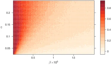
Having verified convergence, we focus on the limit behavior of our algorithms. We find, first of all, that the algorithms consistently learn to charge supracompetitive prices, obtaining a sizable extra-profit compared to the static Nash equilibrium. To quantify this extra-profit, we use the following normalized measure:
(9) Δ ≡ π _______– − π N
π M − π N ,
where π – is the average per-firm profit upon convergence, π N is the profit in the Bertrand-Nash static equilibrium, and π M is the profit under full collusion (monop-oly). Thus, Δ = 0 corresponds to the competitive outcome and Δ = 1 to the per-fectly collusive outcome. Taking π M as a reference point makes sense when δ is sufficiently high that perfect collusion is attainable in a subgame perfect equilib-rium, as is the case in our baseline specification.21 We shall refer to Δ as the average
profit gain.
The average profit gain achieved upon convergence is represented in Figure 1 as a function of α and β . Over our grid, Δ ranges from 70 percent to 90 percent . The corresponding prices are almost always higher than in the one-shot Bertrand-Nash equilibrium but rarely as high as under monopoly (details in online Appendix Section A3.2).
The profit gain does not seem to be particularly sensitive to changes in the learn-ing and experimentation parameters. It tends to be largest when α and β are both low, i.e., exploration is extensive and learning is persistent, but reducing either α or β too much eventually backfires.
21 In fact, the largest attainable Δ is slightly lower than 1 as 𝐩 M can at best be approximated. However, the
difference is immaterial as the profit function is flat at 𝐩 M . On the other hand, Δ can be negative as the action
set includes prices lower than 𝐩 N . In particular, we have Δ ≈ − 2% if the Nash price is approximated by defect,
whereas Δ ≈ 12% if it is approximated by excess.
Table 1—Descriptive Statistics
Sessions by cycle length Nash
equilibria
1-Sym. 1-Asym. 1 2 ≥ 3 All
Frequency 0.277 0.366 0.643 0.238 0.119 1 0.505
Average profit gain 0.866 0.855 0.860 0.846 0.793 0.849 0.854
Standard deviation profit gain 0.115 0.114 0.114 0.104 0.097 0.112 0.108
Frequency of Nash equilibria 0.686 0.661 0.672 0.294 0.025 0.505 1.000
Average Q-loss (on path) 0.001 0.001 0.001 0.002 0.004 0.002 0.000
Standard deviation Q-loss (on path) 0.002 0.004 0.003 0.003 0.006 0.004 0.000
Average Q-loss (all states) 0.018 0.018 0.018 0.018 0.018 0.018 0.018
D. Equilibrium Play
Even if the algorithms almost always converge to a limit strategy, this may not be an optimal response to that of the rival. Optimality is guaranteed theoretically for single-agent decision-making but not when different algorithms are involved.
But again, this property can be verified ex post. We proceed as follows. In each session, for each algorithm we calculate the theoretical Q-matrix under the assump-tion that the rival uses his limit strategy. This assumpassump-tion serves to pin down the last term in equation (3), producing a system of linear equations that can be solved for the “true” Q-matrix. With these Q-matrices at hand, we then determine the algo-rithms’ optimal strategies, i.e., the best responses to the rival’s limit strategy, and compare them to their own limit strategies. The comparison may be limited to the states that are actually reached on path (verifying whether a Nash equilibrium is played), or extended to all states (verifying subgame perfection). When an algo-rithm is not playing a best response, we can also compute the forfeited payoff. We express this in percentage terms and refer to it as the “ Q-loss.”
Figure 2 plots the frequency of equilibrium play, i.e., the fraction of sessions where both algorithms play a best response to the rival’s limit strategy, on path. Lack of equilibrium is quite common when β is large (that is, exploration is limited). This should not come as a surprise. As noted, when β is close to the upper bound of the grid, exploration is too limited to allow good learning. Nevertheless, even when the algorithms do not play a best response, they are not far from it. Most often, the Q-loss is below 0.5 percent, and in no point of the grid does it exceed 1.2 percent (details in online Appendix Section A3.3).
When experimentation is more extensive (i.e., toward the left side of the grid), equilibrium play becomes much more prevalent. For example, when α = 0.15 and β = 0.4 × 10 −5 (meaning that each cell is visited on average 20 times just by random exploration), about one-half of the sessions produce equilibrium play on path, and the Q-loss is a mere 0.2 percent on average (see Table 1). In many cases, the reason why the algorithms are not exactly optimizing is that they approximate
Figure 1. Average Profit Gain Δ for a Grid of Values of α and β β ×105 α 0.05 0.1 0.15 0.2 0.5 1 1.5 0.7 0.75 0.8 0.85 0.9
the price, which would be the best response in a continuous action space, by excess rather than by defect, or vice versa. A key implication is that once the learning pro-cess is completed, there is very little scope for exploiting the algorithms, no matter how smart the opponent is.22
Off path, things are somewhat different. Very rarely do the algorithms play a subgame perfect equilibrium. Again, this is not surprising, given that the algorithms learn purely by trial and error, and subgame perfection is a very demanding require-ment when the state space is large.23 Nevertheless, with enough experimentation we
observe clear patterns of behavior even off path, as we shall see in the next section. Summarizing, we have seen that once they are trained, our algorithms consis-tently raise their prices above the competitive level. These supracompetitive prices do not hinge on suboptimal behavior: prices are high even if both algorithms play an optimal strategy, or come quite close to it. In fact, a comparison of Figures 1 and 2 suggests a positive, albeit modest, correlation between profit gain and equilibrium play: to be precise, Pearson’s coefficient of correlation is 0.12 .24
IV. Anatomy of Collusion
In this section, we analyze the strategies that generate the anticompetitive out-comes described above. A natural question that arises when prices exceed the Nash-Bertrand level is why firms do not cut their prices. Is it because they are miss-ing an opportunity to increase their payoff? Or is it because they realize that cuttmiss-ing the price would not be profitable given the rival’s response in subsequent periods?
22 In the computer science literature, the Q-loss is indeed called “exploitation.” Whether Q-learning algorithms can be exploited during the learning phase is an interesting question for future study.
23 However, Table 1 shows that the algorithms are not far from optimizing even off path, with an average Q-loss of less than 2 percent for the chosen experiment (details in online Appendix Section A3.3).
24 The correlation is even higher, i.e., 0.24 , if equilibrium play is measured by the fraction of cases in which at least one algorithm is playing a best response to the rival’s limit strategy.
Figure 2. Fraction of Sessions Converging to a Nash Equilibrium, for a Grid of Values of α and β
α 0.05 0.1 0.15 0.2 0.5 1 1.5 0 0.2 0.4 0.6 0.8 β ×105
And in this latter case, what would that response look like? These are the questions addressed in what follows.
To ease the exposition, we shall often focus on one point of the grid, namely α = 0.15 and β = 4 × 10 −6 but the results are robust to changes in these parameters. With these parameter values, for each cell we have on average about 20 updates just by random exploration (i.e., ν ≈ 20 ), so even for cells that are visited purely by chance, the initial Q-value counts for just 3 percent of their final value.
Table 1 reports various descriptive statistics for the experiment chosen, both jointly for all sessions and separately for those that converged to a symmetric price, to asymmetric prices (but still constant over time), or to cycles of differing length. The last column focuses instead on those sessions in which the algorithms have learned to play a Nash equilibrium. Two remarks are in order. First, while in almost all sessions the algorithms manage to coordinate, the exact form of the coordination varies. For example, even if the algorithms are fully symmetric ex ante, only in little more than one-fourth of the sessions do they end up charging exactly the same price period after period. All the other sessions display either asymmetries or cycles, or both. Second, the cycles are associated with less equilibrium play and lower profit gain. This is true to a lesser extent for cycles of period 2, which could be interpreted as orbits around a target that is not feasible because of our discretization.25 However,
for cycles of period 3 or longer the effects are quite significant. These cycles, which might reflect the difficulty of achieving coordination purely by trial and error, are not very frequent, however: they materialize in about one-tenth of the sessions.
A. Competitive Environments
Before inquiring into how cooperation is sustained, we show that the algorithms learn to price competitively, at least approximately, when this is the only rational strategy. In particular, collusion is not feasible when k = 0 (the algorithms have no memory and thus cannot punish deviations), and it cannot be an equilibrium phenomenon when δ = 0 (the algorithms are short-sighted and thus the immediate gain from defection cannot be outweighed by any loss due to future punishments).
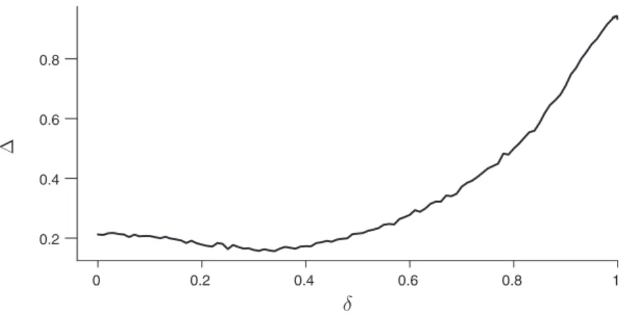
Consider first what happens when the algorithms are short-sighted. Figure 3 shows how the average profit gain varies with δ . The theoretical postulate that lower discount factors impede collusion is largely confirmed by our simulations. The profit gain indeed decreases smoothly as the discount factor falls, and when δ = 0.35 it has already dropped from over 80 percent to a modest 16 percent.26(To appreciate
this value, remember that with our discretization of the price space, the average profit gain would already be close to 12 percent if the Nash-Bertrand prices were just approximated by excess rather than by defect.)
At this point, however, something perhaps surprising happens: the average profit gain turns back up as δ decreases further. Although the increase is small, it runs 25 For period-2 cycles, the fall in the profit gain is indeed small. As for equilibrium play, the decrease is more substantial but in part it may be due to the mechanical effect of doubling the number of states that are reached on path.
26 The fall in Δ actually starts well before δ gets so low that the monopoly outcome is no longer attainable in a subgame perfect equilibrium. With grim-trigger strategies, for instance, the critical threshold of δ is about 40 percent for our baseline specification.
counter to theoretical expectations. We believe that this “paradox” arises because changing δ affects not only the relative value of future versus present profits, but also the effective rate of learning. This can be seen from equation (4), which implies that the relative weight of new and old information depends on both α and δ .27 In
partic-ular, a decrease in δ tends to increase the effective speed of the updating, which as noted may impede learning when exploration is extensive.28 At any rate, the profit
gain remains small.
For the case of memoryless algorithms, we again find modest profit gains, only slightly higher than what is entailed by the discretization of the action space (details in online Appendix Section A4.1). All of this means that our algorithms learn to play, approximately, the one-shot equilibrium when this is the only equilibrium of the repeated game. If they do not price so competitively when other equilibria exist, it must be because they have learned other, more sophisticated strategies.
B. Deviations and Punishments
Providing a complete description of these strategies is not straightforward. The problem is not that they must somehow be inferred from observed behavior, as is typically the case in experiments with humans. Here, at any stage of the simulations we know exactly not only what the algorithms do but also what they would do in any possible circumstances. The difficulty lies instead in the description of the strat-egies. For one thing, strategies are complicated objects (in our baseline experiment, they are mappings from a set of 225 elements to a set of 15 elements). For another, the limit strategies display considerable variation from session to session, and aver-aging masks relevant information.
27 Loosely speaking, new information is the current reward π
t , and old information is whatever
informa-tion is already included in the previous Q-matrix, 𝐐 t−1 . The relative weight of new information in a steady state where Q = π/(1 − δ) then is α (1 − δ) .
28 A similar problem emerges when δ is very close to 1. In this case, we observe that the average profit gain eventually starts decreasing with δ . This reflects a failure of Q-learning for δ ≈ 1 , which is well known in the computer science literature.
0 0.2 0.4 0.6 0.8 1 0.2 0.4 0.6 0.8 δ 4
Figure 3. The Average Profit Gain Δ as a Function of the Discount Factor δ in Our Representative Experiment
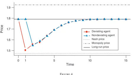
We therefore start by asking, specifically, whether unilateral price cuts are prof-itable in view of the rival’s reaction. To this end, we focus once again on the algo-rithms’ limit strategies. As discussed above, these generally entail supracompetitive prices. Starting, in period τ = 0 , from the prices the algorithms have converged to, we step in and exogenously force one algorithm to defect in period τ = 1 . The other algorithm instead continues to play according to his learned strategy. We then examine the behavior of the algorithms in the subsequent periods, when the forced cheater reverts to his learned strategy as well.
Figure 4 shows the average of the impulse-response functions derived from this exercise for all 1,000 sessions of our representative experiment.29 It shows the
prices chosen by the two agents after the deviation. In particular, Figure 4 depicts the evolution of prices following a one-period deviation to the static best-response to the rival’s predeviation price.30
Clearly, the deviation gets punished. As Table 3 shows, in more than 95 percent of the cases the punishment makes the deviation unprofitable; that is, “incentive compatibility” is verified.
The dynamic structure of the punishment is very interesting. After an initial price war, the algorithms gradually return to their predeviation behavior. This pattern looks very different from the one that would be implied, for instance, by grim-trigger strategies.31 These latter strategies, which are the workhorse of many
theoretical analyses of collusion, are never observed in our experiments. The reason for this is simple: with experimentation, one algorithm would sooner or later defect, 29 When the algorithms converge to a price cycle, we consider deviations starting from every point of the cycle and take the average of all of them.
30 We have also considered the case of an exogenous deviation that lasts for 5 periods. The dynamic pattern is similar to that of one-period deviations (details in online Appendix Section A4.2).
31 Strictly speaking, grim-trigger strategies require unbounded memory, but it is easy to define their one-period memory counterpart.
Figure 4
Notes: Prices charged by the two algorithms in period τ after an exogenous price cut by one of them in period τ = 1 . The forced cheater deviates to the static best response, and the deviation lasts for one period only. The figure plots the average prices across the 1,000 sessions. For sessions leading to a price cycle, we consider deviations starting from every point of the cycle and take the average of all of them. This counts as one observation in the calculation of the overall average.
1.5 1.6 1.7 1.8 1.9 Time Price 0 1 5 10 15 Deviating agent Nondeviating agent Nash price Monopoly price Long-run price
and when this happened both would be trapped in a protracted punishment phase that would last until further (joint) experimentation drove the firms out of the trap. Our algorithms, by contrast, consistently learn to restart cooperation after a devi-ation. This seems necessary in an environment characterized by extensive experi-mentation, where coordination would inevitably be disrupted if it were not robust to idiosyncratic shocks.32
The pattern of punishment we observe is more similar to the “ stick-and-carrot” strategies of Abreu (1986). However, there are differences with Abreu’s strategies as well: the initial punishment is not as harsh as it could be (prices remain well above the static Bertrand-Nash equilibrium), and the return to the predeviation prices is gradual rather than abrupt.
To show that the pattern depicted in Figure 4 is not an artifact of the averaging, Figure 5 reports more information on the distribution of the impulse responses.33
While there is considerable variation across sessions, especially in the first periods after the deviation, the pattern is robust. (See also the fan chart in online Appendix Section A4.2.)
Figures 4 and 5 focus on deviations that maximize the short-run gain from defec-tion. However, we have performed the same type of exercise for all possible price cuts. Table 2 reports the prices charged by the two algorithms immediately after the defection (i.e., in period τ = 2 ). The initial punishment tends to be slightly harsher for bigger price reductions, but the effect is small and nonsystematic. What is sys-tematic is the return to the initial prices; in most of the cases, the punishment ends after 5–7 periods. (See online Appendix Section A4.2.) Table 3 shows that these deviations, too, are almost always unprofitable.
32 This is not a foregone conclusion, however, as the algorithms may start to cooperate only after experimenta-tion had already faded away. That cooperaexperimenta-tion begins earlier is confirmed by the analysis in Secexperimenta-tion VI.
33 Here we restrict attention to sessions that converge to constant prices to avoid spurious effects that may arise because of the averaging across different initial conditions.
Figure 5
Notes: For each period τ , the figure shows the mean (black line), the twenty-fifth and seventy-fifth percentiles (shaded rectangles), and the ranges (dashed intervals) of the prices charged after an exogenous price cut in period τ = 1 . To be precise, the variable on the vertical axis is the difference between the current and the long-run price.
0 1 2 3 4 5 6 7 8 9 10 −0.4 −0.3 −0.2 −0.1 0 0.1 Deviating agent Time 0 1 2 3 4 5 6 7 8 9 10 Time Price change −0.4 −0.3 −0.2 −0.1 0 0.1 Price change Nondeviating agent
Table 2—Price Changes after Deviation Preshock
price Frequency
Deviation price
1.43 1.51 1.58 1.66 1.74 1.82 1.89
Panel A. Relative price change by the nondeviating agent in period τ = 2
1.62 0.01 −0.04 −0.07 −0.08 1.66 0.06 −0.08 −0.09 −0.08 0 1.70 0.11 −0.10 −0.10 −0.10 −0.10 1.74 0.16 −0.11 −0.12 −0.12 −0.11 0 1.78 0.19 −0.13 −0.13 −0.13 −0.13 −0.13 1.82 0.18 −0.15 −0.14 −0.14 −0.14 −0.14 0 1.85 0.11 −0.16 −0.17 −0.16 −0.15 −0.15 −0.15 1.89 0.09 −0.18 −0.17 −0.16 −0.16 −0.17 −0.17 0 1.93 0.05 −0.19 −0.19 −0.19 −0.18 −0.18 −0.18 −0.16 1.97 0.03 −0.19 −0.21 −0.21 −0.18 −0.17 −0.18 −0.17
Panel B. Relative price change by the deviating agent in period τ = 2 with respect to τ = 1
1.62 0.01 0.06 0.04 −0.05 1.66 0.06 0.07 0.01 −0.02 0 1.70 0.11 0.08 0.04 −0.02 −0.07 1.74 0.16 0.09 0.03 −0.01 −0.05 0 1.78 0.19 0.09 0.03 −0.02 −0.05 −0.11 1.82 0.18 0.09 0.04 0.00 −0.05 −0.09 0 1.85 0.11 0.09 0.03 −0.01 −0.04 −0.09 −0.12 1.89 0.09 0.10 0.03 0.00 −0.04 −0.08 −0.12 0 1.93 0.05 0.10 0.05 0.01 −0.04 −0.09 −0.11 −0.16 1.97 0.03 0.13 0.07 0.00 −0.02 −0.06 −0.11 −0.13
Notes: To save space, the table reports one of every two deviation prices. The full table is in online Appendix Section A4.2. Table 3—Unprofitability of Deviations Preshock price Frequency Deviation price 1.43 1.51 1.58 1.66 1.74 1.82 1.89
Panel A. Average percentage gain from the deviation in terms of discounted profits
1.62 0.01 −0.03 −0.02 −0.02 1.66 0.06 −0.02 −0.02 −0.02 0 1.70 0.11 −0.03 −0.03 −0.03 −0.03 1.74 0.16 −0.03 −0.03 −0.03 −0.03 0 1.78 0.19 −0.04 −0.03 −0.03 −0.03 −0.03 1.82 0.18 −0.04 −0.04 −0.03 −0.03 −0.04 0 1.85 0.11 −0.04 −0.04 −0.03 −0.03 −0.03 −0.04 1.89 0.09 −0.04 −0.04 −0.03 −0.03 −0.03 −0.04 1.93 0.05 −0.04 −0.04 −0.03 −0.03 −0.03 −0.03 −0.04 1.97 0.03 −0.04 −0.03 −0.03 −0.03 −0.03 −0.03 −0.03
Panel B. Frequency of unprofitable deviations
1.62 0.01 1.00 0.91 0.91 1.66 0.06 1.00 0.95 0.95 0 1.70 0.11 0.99 0.99 0.98 0.98 1.74 0.16 0.99 0.97 0.95 0.95 0 1.78 0.19 0.99 0.98 0.96 0.98 0.98 1.82 0.18 0.99 0.98 0.99 0.97 0.98 0 1.85 0.11 0.99 0.97 0.97 0.99 0.96 0.97 1.89 0.09 0.98 0.97 0.95 0.97 0.96 0.97 0 1.93 0.05 0.99 1.00 0.93 0.97 0.99 0.97 0.96 1.97 0.03 1.00 1.00 0.97 0.88 0.91 0.94 0.94
Notes: To save space, the table reports one of every two deviation prices. The full table is in online Appendix Section A4.2.
For example, consider a preshock price of 1.78 (this is the tenth price of the grid, and it accounts for almost 20 percent of the cases where both algorithms converged to the same price). Table 2 shows that, irrespective of the size of the rival’s exoge-nous deviation in period τ = 1 , the nondeviating algorithm would cut the price in period τ = 2 by approximately the same percentage amount (i.e., 13 percent, lead-ing to a price of approximately 1.54). The deviating algorithm, in contrast, raises his price if the deviation was big and further lowers the price if the deviation was small, pricing on average just above its rival.34 Table 3 shows that even if the algorithms
manage to restart cooperation pretty soon, the deviation reduces the forced cheater’s discounted profits by 3–4 percent on average. Only in a tiny fraction of the cases the deviation is profitable.
For small price cuts, the pattern just described represents a form of overshooting: that is, both algorithms cut their prices further in period τ = 2 , below the exoge-nous initial reduction of period τ = 1 . This is illustrated in Figure 6, which shows the average impulse-response corresponding to one of these smaller deviations. The overshooting would be difficult to rationalize if what we had here was simply a sta-ble dynamic system that mechanically returns to its rest point after being perturbed. But it makes perfect sense as part of a punishment.
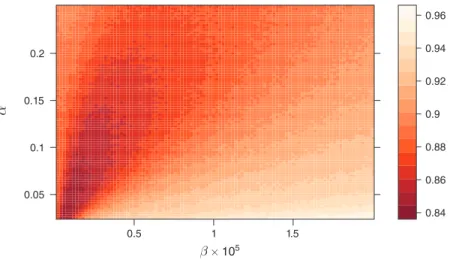
As mentioned, these results do not depend on the specific values chosen for α and β : we observe punishment of deviations over the entire grid considered in the previous section. To illustrate, Figure 7, plots an index of the intensity of the punishment (i.e., the average percentage price cut of the nondeviating agent in period τ = 2 ) as a function of α and β . The figure confirms that punishment is ubiquitous. The harshness of the punishment is strongly correlated with the profit gain: the coefficient of correlation is 76.2 percent . This is one more sign that the supracompetitive prices are the result of genuine tacit collusion.
C. The Graph of Strategies
Let us now face the problem of describing the limit strategies more fully. Generally speaking, with a one-period memory strategies are mappings from the past prices
(
p 1,t−1 , p 2,t−1)
to the current price p i,t : p i,t = F i(
p 1,t−1 , p 2,t−1)
. In our experiments, thealgorithms systematically coordinate on one pair of prices (or a cycle) and punish any move away from the agreed upon prices. However, these prices vary from ses-sion to sesses-sion, and the intensity of the punishment is variable as well, depending rather capriciously on the distance from the long-run prices. For this reason, one cannot derive a representative strategy by simply averaging across different func-tions F i (details in online Appendix Section A5.3).35
One obvious way to work around this problem would be to average only across those sessions where the algorithms converge to the same pair of supracompetitive prices. In this case, the average function F must obviously exhibit a spike at that point. Elsewhere prices must be much lower, reflecting the punishment of deviations.
34 It is tempting to say that the deviating algorithm is actively participating in its own punishment. At the very least, the deviating algorithm is anticipating the punishment: otherwise it would have no reason to reduce its price as soon as it regains control, i.e., in period τ = 2 , given that the rival’s price was still high in period τ = 1 .
But apart from these obvious properties, even such conditional averages display no recognizable pattern.
Evidently, there is considerable variation not only in the prices on which the algorithms converge to but also in their limit behavior off path. In other words, the exact way the algorithms achieve coordination depends on the specific history of their interactions. One could not, perhaps, expect anything else from agents that learn purely by trial and error.
This suggests that limit strategies may be better studied in pairs, looking at the combined behavior of those algorithms that interacted with one another. This com-bined behavior may be described using the directed graph produced by any pair of
Figure 6
Notes: This figure is similar to Figure 4, except that the exogenous price cut is smaller. As a result, prices fall further down in period τ = 2. In other words, the impulse-response function exhibits “overshooting.”
1.5 1.6 1.7 1.8 1.9 Time Price 0 1 5 10 15 Deviating agent Nondeviating agent Nash price Monopoly price Long-run price
Figure 7. Average Percentage Price Reduction by the Nondeviating Agent in Period τ = 2 , for a Grid of Values of α and β
β × 105 α 0.05 0.1 0.15 0.2 0.5 1 1.5 0.84 0.86 0.88 0.9 0.92 0.94 0.96
strategies. For example, Figure 8 depicts the graph of the limit strategies obtained in one session of our representative experiment. In any graph like this, the node corresponding to the long-run prices (which is marked as a square in the figure) is absorbing.36
The graph is quite complex but exhibits a few remarkable properties. First and foremost, all the nodes eventually lead to the absorbing node. This means that the algorithms systematically restart cooperation not only after unilateral but also after bilateral deviations. Second, there are a few key nodes that act as gateways, either directly or indirectly, to the absorbing node. Third, the paths to the absorbing node are generally rather short: the average length of the path is 6, and the maximum length is 18. Online Appendix Section A4.3 shows that the properties exhibited by this example are in fact much more general. For example, in 92 percent of the
36 For sessions that converge to a price cycle, the system would cycle around two or more nodes. Figure 8
Notes: The directed graph of the limiting strategies in one session of the representative experiment. The absorbing node (corresponding to the long-run prices) is represented by the square, all other nodes by circles. The brightness of the nodes represents the profit gain (the darker the node, the higher the profit gain), while the size represents the node’s centrality (as measured by betweenness centrality).
sessions the system converges to the long-run prices starting from any possible node; and in 98 percent of the sessions there are fewer than 3 nodes, out of 225, that do not eventually lead to the long-run prices.
Figure 9 represents, for the same example, the limit strategies in a way that facil-itates the economic interpretation of the nodes. Nodes are ordered according to the level of the prices charged by algorithm 1 (horizontal axis) and 2 (vertical axis). The arrows starting from each node indicate the direction of the price change, but to make the figure easier to read they do not extend as far as the next node that is reached. The figure shows that starting from any node other than the absorbing one, the system initially moves toward the low part of the main diagonal and then climbs up to the long-run prices. This suggests that cooperation does not restart immedi-ately but only after a punishment phase, and that bilateral deviations are punished in pretty much the same way as unilateral deviations.
V. Robustness
How robust are our baseline results to changes in the economic environment? In this section, we consider a number of factors that may affect firms’ ability to sustain a tacit collusive agreement. Throughout, we continue to focus on our chosen values for the learning and experimentation parameters, α = 0.15 and β = 4 × 10 −6 . The supplementary material file provides more details and presents several other robustness exercises.
A. Number of Players
Theory predicts that collusion is harder to sustain when the market is more frag-mented. We find that, indeed, the average profit gain Δ decreases from 85 percent to 64 percent in simulations with three firms. With four agents, the profit gain is still a substantial 56 percent. The decrease in the profit gain seems slower than in experi-ments with human subjects.37
These results are all the more remarkable because the enlargement of the state space interferes with learning. Indeed, moving from n = 2 to n = 3 or n = 4 enlarges the Q-matrix dramatically, from 3,375 to around 50,000 or over 750,000 entries. Since the parameter β is held constant, the increase in the size of the matrix makes the effective amount of exploration much lower. If we reduce β so as to com-pensate for the enlargement of the matrix, at least partially, the profit gain increases. For example, with three firms we find values of Δ close to 75 percent.38
The impulse-response functions remain qualitatively similar to the case of duopoly. We still have punishments, which however tend to be more prolonged and generally harsher than in the two-firms case.
37 The early experimental literature indeed found that in the lab, tacit collusion is “frequently observed with two sellers, rarely in markets with three sellers, and almost never in markets with four or more sellers” (Potters and Suetens 2013, p. 17). More recently analyses paint a more nuanced picture, though. In some experiments, three or four human subjects manage to achieve levels of coordination comparable to our algorithms: see Horstmann, Krämer, and Schnurr (2018) and Friedman et al. (2015).
38 In order to make the learning process more effective, the increase in the amount of experimentation is matched by a decrease in the learning rate. The increase in the profit gain goes hand in hand with the increase in the frequency of equilibrium play.
B. Asymmetric Firms
The conventional wisdom has it that asymmetry impedes collusion. Firms con-templating a tacit collusive agreement must solve a two-fold problem of coordina-tion: they must choose both the average price level, which determines the aggregate profit, and the relative prices, which determine how the total profit is split among the firms. Achieving coordination on both issues without explicit communication is often regarded as a daunting task.
To see how Q-learning algorithms cope with these problems, we considered both cost and demand asymmetries of different degrees. Table 4 reports the results for the case of cost asymmetry (the case of demand asymmetry is similar and reported in online Appendix Section A5.2).
As the table shows, asymmetry does reduce the average profit gain, but only to a limited extent. In part the decrease is simply a consequence of the absence of side payments. To see why this is so, consider how the two algorithms divide the aggregate profit. As the last row of the table shows, the gain from collusion is split disproportionately in favor of the less efficient firm.
Figure 9
Notes: Phase portrait of the limiting strategies. The Bertrand-Nash price is best approximated by the third lowest price, the monopoly price by the third highest. Form, size, and brightness of the nodes are as in Figure 8.