Università degli Studi della Calabria
Dottorato di Ricerca in Ingegneria Chimica e dei Materiali
Tesi
Modellistica di membrane polimeriche “high performance”
per separazione di gas
Settore Scientifico Disciplinare CHIM07 – Fondamenti chimici delle tecnologie
Supervisori Candidato
Dr. Elena TOCCI Luana De Lorenzo
Dr. Giovanni GOLEMME Ciclo XXII
Il Coordinatore del Corso di Dottorato Ch.mo Prof. Raffaele MOLINARI
A.A. 2008-2009
Fondo Sociale Europeo - FSE Programma Operativo Nazionale 2000/06 "Ricerca, Sviluppo tecnologico ed Alta Formazione
Ma guardate l'idrogeno tacere nel mare guardate l'ossigeno al suo fianco dormire: soltanto una legge che io riesco a capire ha potuto sposarli senza farli scoppiare.
Introduzione Generale
Università degli studi della Calabria – Tesi di Dottorato – A.A. 2008/2009 – Luana De Lorenzo I
INTRODUZIONE GENERALE
1. Definizione del problema.
Vi è un notevole interesse verso lo studio del trasporto di piccole molecole attraverso membrane polimeriche, soprattutto a causa del gran numero di applicazioni in cui tale processo di trasporto svolge un ruolo importante.
Le membrane polimeriche sono principalmente utilizzate come : membrane per separazione.
involucri plastici .
Queste due applicazioni richiedono membrane con caratteristiche completamente diverse. Per la prima applicazione è importante che il materiale polimerico sia altamente selettivo e sufficientemente permeabile, mentre per la seconda la membrana deve avere un'elevata resistenza a gas o a sapori-aromi.
L’interesse per tali applicazioni industriali ha stimolato lo sviluppo di modelli teorici per descrivere il processo di trasporto. Esiste un gran numero di modelli, ciascuno dei quali, tuttavia, manca di una corretta descrizione microscopica del processo di permeazione. Metodi di simulazione al computer e, in particolare, simulazioni di dinamica molecolare rappresentano uno strumento essenziale per ottenere un quadro più dettagliato di tali fenomeni. Una descrizione qualitativa dei processi descritti e infine le previsioni quantitative di permeabilità e selettività aprono la strada alla prospettiva di progettare membrane con specifiche caratteristiche. Al momento non siamo ancora nella fase delle previsioni. La maggior parte degli studi in questo momento sono interessati a descrivere la diffusione e il processo di permeazione e si limitano al confronto con i dati sperimentali ottenuti per membrane già esistenti.
La presente tesi descrive un progetto di ricerca in questo settore di rapida evoluzione.
2. Scopo della ricerca
L'obiettivo del progetto di ricerca oggetto della presente tesi di dottorato è quello di studiare le proprietà di trasporto di piccole molecole attraverso membrane polimeriche utilizzando metodi teorici di simulazione al fine di ottenere utili correlazioni struttura-proprietà.
Sono stati scelti per essere studiati con il metodo di Dinamica Molecolare (MD) due diversi tipi di materiali per le loro alte prestazioni come materiali di membrane per separazioni gassose.
In particolare, le simulazioni a livello atomistico sono state utilizzate per investigare: • il processo di trasporto di gas e vapori e l'analisi strutturale di copolimeri gommosi puri e modificati caratterizzati da alta selettività per gas polar / non polari: la modifica in situ di
Introduzione Generale
tali tipi di membrane con l'aggiunta di percentuali variabili di additivi chimici ne potenzia la permeabilità e la selettività per specifiche applicazioni in campo di separazione gassosa.
• le caratteristiche morfologiche di polimeri vetrosi ad elevato volume libero e altamente permeabili, recentemente utilizzati per separazioni di gas complicate (ad esempio, di olefine/ paraffine o trattamento di gas naturale), attraverso la misura quantitativa della distribuzione del volume libero.
Al di là di una convalida reciproca tra dati sperimentali e teorici, una delle questioni più importanti della ricerca computazionale sui materiali di membrana è la simulazione multiscala, vale a dire il collegamento tra vari metodi di calcolo che si sviluppano in diverse scale di lunghezza e di tempo per prevedere le proprietà macroscopiche e il comportamento di fondamentali processi molecolari. L'idea alla base della modellazione multiscala è di facile comprensione: si calcolano informazioni più dettagliate su scale ridotte per passare a modelli meno dettagliati su scale superiori. L'obiettivo finale della modellazione multiscala è quindi di prevedere il comportamento macroscopico di un processo ingegneristico da principi primi, cioè, a partire dalla scala quantistica attraverso la trasmissione di informazioni in scala molecolare fino al processo.
Andando nella direzione di un approccio multidisciplinare e di interconnessione di metodi matematici di modellazione nel corso del progetto di ricerca simulazioni mesoscale (utilizzando la teoria dinamica del campo medio (DDFT) e la dinamica dissipativa delle particelle (DPD) tramite modelli molecolari coarse-grained) sono state effettuate per studiare la morfologia di copolimeri a blocchi di interesse nel settore della nanotecnologia.
3. Scelta dei polimeri
I materiali scelti sono:
• PEBAX ® 2533: un copolimero ad alta percentuale di contenuto gommoso della serie di poli(amide-12b-etilenossido) nota con il nome di PEBAX.
• HYFLON®AD60X e HYFLON® AD80X: perfluoropolimeri vetrosi.
Entrambi i materiali sono comunemente utilizzati per la preparazione di membrane dense e sono caratterizzati da alte prestazioni nella separazione di gas.
4. Sommario della tesi
Capitolo 1: Membrane per la separazione di gas. Questo capitolo fornisce una panoramica generale sui diversi tipi di membrane polimeriche, con particolare attenzione alle membrane e ai processi di separazione gassosa. Vengono mostrati e descritti nel dettaglio le principali equazioni e i metodi di misura delle proprietà di trasporto dei gas attraverso membrane polimeriche.
Capitolo 2: Basi teoriche di simulazione molecolare. Questo capitolo descrive i principi di base della tecnica di Dinamica molecolare e i metodi usati per calcolare diffusività, solubilità e volume libero.
Capitolo 3: Proprietà di trasporto di membrane di poli(amide-12-b-etilenossido) (PEBAX); in questo capitolo viene descritto in dettaglio lo studio atomistico del meccanismo
Introduzione Generale
Università degli studi della Calabria – Tesi di Dottorato – A.A. 2008/2009 – Luana De Lorenzo III
di trasporto di gas polari-non polari attraverso membrane di poli (etere /ammide). Vengono inoltre fornite utili correlazioni struttura microscopica /proprietà di trasporto, sottolineando il ruolo delle selettività di diffusività e di solubilità per diverse specie penetranti.
Capitolo 4: Proprietà di trasporto dell’acqua in membrane modificate di PEBAX: questo capitolo descrive le indagini MD di proprietà di trasporto dell'acqua attraverso sistemi PEBAX modificati con diverse percentuali in peso di toluensulfonamide (KET). Vengono fornite inoltre utili correlazioni tra la struttura microscopica dei materiali oggetto di studio e le prestazioni di questi sistemi in termini di diffusività e solubilità dell’acqua sperimentalmente misurate.
Capitolo 5: Indagini molecolare delle proprietà di trasporto di gas e vapori in membrane
di PEBAX modificate. Questo capitolo fornisce una dettagliata descrizione delle simulazioni
atomistiche del trasporto di H2O, N2, O2, CO2, CH4 attraverso i materiali oggetto di studio per
valutare la selettività tra specifiche coppie di gas e il confronto con i dati sperimentali.
Capitolo 6: Simulazione mesoscala della morfologia e delle proprietà di trasporto in
membrane di PEBAX. In questo capitolo viene descritta la procedura mesoscala usata per
studiare la complessa morfologia del PEBAX®2533, con una breve descrizione dei metodi DDFT e DPD. Vengono presentati i risultati preliminari e delineate le prospettive future.
Capitolo 7: Analisi delle distribuzioni di volume libero in perfluoropolimeri amorfi. Questo capitolo fornisce una descrizione dettagliata della procedura MD per il calcolo del volume libero in films di amorfi perfluoropolimeri vetrosi di HYFLON®AD60x e AD80x e il confronto con i risulatti ottenuti da vari metodi sperimentali.
General Introduction
GENERAL INTRODUCTION
1. Problem definition
There is a considerable interest in the study of the transport of small molecules across polymeric membranes, mainly because of the large number of applications in which this transport process plays a major role.
Polymeric membranes are mainly used as: separation membranes.
barrier plastics.
These two applications require membranes with completely different properties. In the first application it is important that the polymeric material is highly selective and sufficiently permeable, while in the second application the membrane should have high resistance to gas and e.g. flavor-aroma molecules.
Such interest has stimulated the development of theoretical models to describe the transport process. There are a large number of models, all of which, however, lacks a complete microscopic description of the permeation process. Computer simulation methods and in particular molecular dynamics simulations are an essential tool to obtain a more detailed picture of these phenomena. A qualitative description of the underlying processes and eventually quantitative predictions of permeability and selectivity open the prospect to the design of membranes with tailored properties. At present we are not yet at the stage of predictions. Most studies at this moment are concerned with describtion of the diffusion and the permeation process and are restricted to comparison with existing membranes.
This thesis describes one study in this fast moving field of research.
2. Aim of the research
The aim of this research is to study the transport properties of small molecules through polymeric membranes using computer simulation methods and to obtain useful correlations with the microstructure properties.
Two different types of materials are been chosen to be investigated by Molecular Dynamics (MD) method due to the high performances for gas separation exhibited in the field of membrane technology.
In particular fully atomistic simulations have been used to study:
Gases and vapour transport and structural analysis of pure and modified rubbery copolymer with high selectivity for polar/non polar gases; the modification in situ of these types of membranes by adding variable percentages of chemical additives led to an enhancement of specific surface and permeability properties.
Morphological properties of high free volume glassy perfluoropolymers, recently used for challenging gas separations (e.g., olefin/paraffin or natural gas treatment), by quantitative measure of free volume distributions.
General Introduction
Beyond a reciprocal validation between experimental and theoretical data, one of the most important issue in computational materials research is the multiscale simulation, namely the bridging of length and time scales, and the linking of computational methods to predict macroscopic properties and behavior from fundamental molecular processes. The idea of multiscale modeling is straightforward: one computes information at a smaller (finer) scale and passes it to a model at a larger (coarser) scale by leaving out, i.e., coarse-graining, degrees of freedom. The ultimate goal of multiscale modeling is then to predict the macroscopic behavior of an engineering process from first principles, i.e., starting from the quantum scale and passing information into molecular scales and eventually to process scales.
Going in the direction of a multidisciplinary approach and interconnections of mathematical theorical method in the present research Mesoscale simulations (Dynamic mean field theory (Mesodyn) and dissipative particle dynamics (DPD) utilizing coarse-grained molecular models) are been used for investigating the morphology of block copolymers for nanotechnologycal applications.
3. Choice of polymers
The chosen materials are:
PEBAX®2533: an almost totally rubbery copolymer of the Poly(amyde-12b-ethylene
oxide) PEBAX series.
Hyflon ®AD60X and Hyflon AD80X: glassy perfluoropolymers.
Both the materials are commonly used in the preparation of dense membrane and exhibited high performance in the field of gas separation.
4. Outline of the thesis
Chapter 1: Membranes for gas separation. This chapter is a general overview about the different types of polymer membranes, with particular attention for the gas separation membranes and processes. The main equations related to the gas transport properties and their measurements are also shown and described.
Chapter 2: Theoretical basis of Molecular simulation; this chapter describes the basic principles of the technique of molecular dynamics and the method for calculating diffusivity, solubility and free volume.
Chapter 3: Transport properties of a copoly(amide-12-b-ethyleneoxide) (PEBAX)
membrane; in this chapter a detailed fully-atomistic investigation of the separation of
polar/non polar pair gas through co-poly(ether/amide) block membranes has been provided. An assessment of the structure/property relationships is included, highlighting the role of diffusivity and solubility selectivities for various penetrant species.
Chapter 4: Water Transport properties of modified PEBAX membranes: this chapter describes the MD investigations of water transport properties across PEBAX systems with different weight percentage of the additive toluensulphonamide (KET); useful correlations
General Introduction
between the microscopic structure of the materials object of study and the performances of these systems in terms of water diffusivity and solubility have been provided.
Chapter 5: Molecular investigations of gas and vapours transport properties in modified
PEBAX membrane: in this chapter a fully atomistic study has been performed for simulating
the transport of H2O, N2, O2, CO2, CH4 for evaluating the selectivity between specific couple
of gases and compared with experimental data.
Chapter 6: Mesoscale Simulation of morphology and transport properties in PEBAX
membrane: in this chapter the mesoscale procedure used for the investigations of complex PEBAX®2533 morphology has been described, with a briefly introduction of DDFT and DPD model equations; preliminary results and future perspectives have been discussed.
Chapter 7: Analysis of the free volume distributions in amorphous glassy
perfluoropolymers: the present paper describes the MD procedure for the free volume
investigation in amorphous glassy perfluoropolymer films of Hyflon ®AD60x and AD80x; the
theoretical data are compared with experimental ones obtained by several experimental techinques.
CHAPTER I - Membrane for gas separation
I. MEMBRANE FOR GAS SEPARATION
1. Basic Principles and Applications
Membrane gas separation process is an important unit operation widely employed in the chemical industries. Membrane-based gas separation offers a number of advantages compared to other traditional methods for certain applications.
Modern membrane engineering is an important way to implement the process intensification (PI) strategy by innovative design and process development methods aimed at decreasing production costs but also equipment size, energy utilization, and waste generation [1.1-1.5]. Membrane science and technology are recognized today as powerful tools in solving some important global problems, developing new industrial processes needed for a sustainable industrial growth. In seawater desalination, membrane operations or their combination in integrated systems are already a successful approach for solving the situation of fresh water demand in many regions of the world, at lower costs and minimum environmental impact. Membranes are a factor of 10 times more energetically efficient than thermal options for water desalination [1.6].
The major production cycles consume as much as 40-50% of the energy used just for separations, often carried out by inefficient thermally driven separation processes.
Membrane gas separation (GS) is a pressure-driven process with different industrial applications that represent only a small fraction of the potential applications in refineries and chemical industries.
Since 1980, when the serial production of commercial polymeric membrane was implemented, membrane GS has rapidly become a competitive separation technology. Differently from conventional separation unit operations (e.g., cryogenic distillation and adsorption processes), membrane GS does not require a phase change. Moreover, the absence of moving parts makes GS systems particularly suited for use in remote locations where reliability is critical; in addition, the small footprint makes them very attractive for remote applications such as offshore gas-processing platforms.
Table 1.1 lists the current status of membrane gas separation processes.
The established processes represent more than 80% of the current gas separation membrane market: nitrogen production from air, hydrogen recovery and air drying. All have been used on a large commercial scale for over 10 years with dramatic improvements in membrane selectivity, flux and process designs. The second group of applications is developing processes which include carbon dioxide separation from natural gas, organic vapour separation from air and nitrogen, and recovery of light hydrocarbons from refinery and petrochemical plant purge gases. Theses processes are being developed on a commercial scale, and the process performance has been improved with the development of better membranes and process designs. In addition, organic vapor separation membranes are currently being developed for petrochemical and refinery applications. The ‘to be developed’ membrane processes represent the future development of gas separation technology. Natural gas treatment by membranes is being carried out at field tests and early commercial stage by several companies. Another large potential application for membranes is the production of
CHAPTER I - Membrane for gas separation
oxygen-enriched air, and the market size is expected to depend largely on the properties of the membranes. [1.7]
CHAPTER I - Membrane for gas separation
Membrane processes are classified according to the driving force by which they achieve separation. The membrane can be simply defined as a permselective barrier that will favour the transport of one component over the others. The separation occurs as a result of the differences in permeabilities of the species through the membrane. In gas separation, when a gas mixture at a pressure higher than the other side contacts a membrane which is selectively permeable to one component of the feed mixture, that species will be enriched on the permeate side.
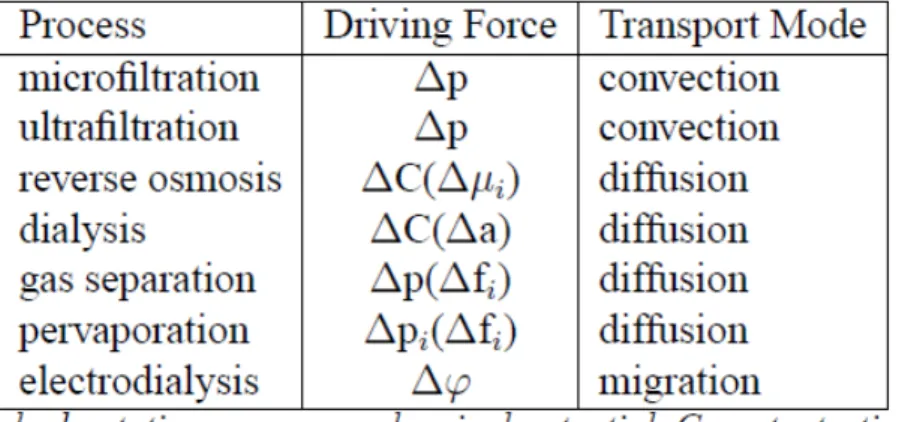
Table 1.2 lists commonly known means of separation along with their primary driving force and type of mechanism.
Table 1. 2-Various membrane separation processes and the corresponding driving forces.
Types of membranes used today include nonporous (dense) and porous polymers, ceramic and metal films with symmetric or asymmetric structures, liquid films with selective carrier components, and electrically charged barriers [1.8].
The performance of a membrane is determined by several key properties: high selectivity and permeability;
excellent chemical, thermal, and mechanical stability under the process operating conditions;
low maintenance; good space efficiency; defect-free production.
Commercially, the most widely practiced separations using membranes include the separation of oxygen and nitrogen; the recovery of hydrogen from mixtures with larger components such as nitrogen, methane and carbon dioxide; and the removal of carbon dioxide from natural gas mixtures. For these separations, membranes with adequately high fluxes of the more permeable components (oxygen, hydrogen, and carbon dioxide, respectively) and sufficient selectivity have been developed. The membrane materials used in these separations
CHAPTER I - Membrane for gas separation
are glassy polymers, which derive high selectivity from their ability to separate gases based on differences in penetrant size
Membranes can be categorized according to their geometry, bulk structure, production method, separation regime, and application [1.9]. Hollow-fiber membranes are used commonly by industries due to their high surface area and compactness. Flat-sheet membranes are easy to produce and are used in laboratory experiments. In terms of structure, membranes can be separated into two groups; asymmetric and symmetric. This simply refers to the types of pores that can be found within the membrane. Symmetric membranes have pores which do not change in diameter significantly through the sheet. On the other hand, asymmetric membranes contain pores which increase in size from one side of the sheet to the other. The new membrane composites are good example of asymmetric membranes. They are made with a thin polymer film deposited onto a porous backing material. The separation is determined by the properties of the thin film while the mass transport or rate is dependent upon the porosity of the backing.
Different production methods can result in membranes with unique characteristics. Membranes are the result of pressing a powder into a porous film and then sintering, stretching an extruded polymer into a sheet, irradiating a thin film with nuclear particles and then etching in a bath (nucleation track), dissolving a polymer in a solvent and spreading into a film followed by precipitation (solution casting), contacting two monomers in two immiscible liquids (interfacial polymerization), or condensing gaseous monomers on a substrate layer through a stimulated plasma (plasma polymerization).
2. Transport through polymer membranes
2.1. Fundamentals
Three general transport mechanisms are commonly used to describe gas separations using membranes, as illustrated in Figure 2.2 [1.10]. They are Knudsen diffusion, molecular sieving, and solution-diffusion. As the name implies, the first type of separation is based on Knudsen diffusion and separation is achieved when the mean free paths of the molecules are large relative to the membrane pore radius. The separation factor from Knudsen diffusion is based on the inverse square root ratio of two molecular weights, assuming the gas mixture consists of only the two types of molecules. The process is limited to systems with large values for the molecular weight ratio, such as is found in H2 separation. Due to their low
selectivities, Knudsen diffusion membranes are not commercially attractive.
The molecular sieving mechanism describes the ideal condition for the separation of vapour compounds of different molecular sizes through a porous membrane. Smaller molecules have the highest diffusion rates. This process can happen only with sufficient driving force.
In other words, the upstream partial pressure of the ”faster” gas should be higher than the downstream partial pressure.
CHAPTER I - Membrane for gas separation
Figure 1. 1 - General transport mechanisms for gas separations using membranes
The main limitation is that condensable gases cause fouling, and alter the structure of the membrane; therefore, it is only feasible commercially in robust systems, such as those that use ultramicroporous carbon or hollow fibre glass membranes.
Solution-diffusion separation is based on both solubility and mobility factors. It is the most commonly used model in describing gas transport in non-porous membranes and it is applied in our studies. The details of this solution-diffusion model are given in the next section.
2.2. Solution_Diffusion Model and Permeability Equations
Gas permeation can be seen as a three-stage process in the solution-diffusion model: 1. adsorption and dissolution of gas at the polymer membrane interface.
2. diffusion of the gas in and through the bulk polymer. 3. desorption of gas into the external phase.
The first to use the term “solution-diffusion mechanism” was Graham [1.9] in 1866. He postulated that the penetrant leaves the external phase by dissolving in the membrane. It then undergoes molecular diffusion in the membrane, driven towards the downstream face by for example a concentration or pressure gradient, after which it evaporates again in the external phase. Thus the permeability coefficient P, defined by the ratio between the flux J of the permeant species and its concentration gradient ∆c over the membrane of thickness d:
d c P
J (1.1)
is given by the product of the diffusion coefficient D and a solubility factor: S
D
CHAPTER I - Membrane for gas separation
A postulate of which the theoretical foundation will be shown next.
In the solution-diffusion model we consider an isothermal homogeneous stationary membrane in which particles at a position r are dissolved with a local concentration c(r).
The particle flux J is assumed to behave in the regime of a linear irreversible process with the gradient of the chemical potential as the driving force. The flux is given by:
) ( ) ( ) (r c r v r J (1.3)
where v(r) is the average velocity of the dissolved particles. In the linear regime v(r) can be written as:
(1.4)
where F is the thermodynamic force, ξ a friction coefficient Δµ(r) and the chemical potential of the dissolved particles. The latter can be written as:
) ( ) ( ln ) (r 0 RT c r r ex (1.5) in which µ0 is the standard chemical potential of the ideal gas phase based on unit molar concentration, c(r) is the local concentration and µex is the excess chemical potential of the
dissolved species with respect to the ideal gas state. The previous equations give:
) ( ) ( ) ( _ ) (r RT c r c r r J ex (1.6)
Equating RT/ ξ with the diffusion coefficient D eq. 1.6 can be written as:
RT r r c RT r D r J( ) exp ex( ) ( )expex( ) (1.7)
Equation 2.7 is still general. We now consider a membrane with thickness d in the x direction and infinite dimensions in the yz-plane. The interfaces at x = 0 are in contact with concentrations c1 and c2 (Δc = c2 – c1) and we assume that an ideal gas phase is in
equilibrium across both interfaces. Hence µ is continuous at the interfaces.
Furthermore µex is assumed to be constant throughout the homogeneous membrane. This
implies that any concentration dependence of µex is neglected. Thus: ex c RT c RT ln 0 ln (0) 1 0 (1.8) or RT c c(0) exp ex 1 (1.9) Similarly ) ( 1 1 ) (r F r v
CHAPTER I - Membrane for gas separation RT c d c( ) exp ex 2 (1.10)
If µex is constant then ∆µex is zero. Then, for a stationary flux we find that according to
equation 1.6, c(x) is a linear function of x and the gradient in equation (1.7) is equal to
d c(0) -(c(d)
. Equation (1.7) now reduces to:
d c S D J (1.11) with: RT S exp ex (1.12)
Equation 1.11 expresses the solution-diffusion mechanism P is permeability of the gas defined as:
S D
P (1.13)
The permeability is a product of the diffusivity and solubility coefficients. Thus, it can be seen that two parameters describe the solution-diffusion model: solubility and diffusivity. The permeability is a product of a thermodynamic factor (the solubility coefficient S ) and a kinetic parameter (the diffusion coefficient D). In real systems, both diffusion and solubility coefficients may be a function of concentration. Selectivity is defined by the ratio of the individual gas permeabilities. Based on pure gas permeabilities, the “ideal selectivity” for gas species “A” and “B” can be defined as:
B A B A B A AB S S D D P P (1.14)
which shows that the overall selectivity is determined by the differences in both the diffusivity and solubility coefficients, and measure the contributions of diffusivity and solubility aspects of the gas permeation, respectively.
Here, DA/DB is the ratio of the concentration-averaged diffusion coefficients of penetrants
A and B, and is referred to as the membrane’s ”diffusivity selectivity”. SA/SB is the ratio of
solubility coefficients of penetrants A and B, and is called the ”solubility selectivity” In typical gas separation applications, the downstream pressure is not negligible; however, αAB
generally provides a convenient measure for assessing the relative ability of various polymers to separate gas mixtures. High permeability and high selectivity are the most important criteria in evaluating a membrane.
CHAPTER I - Membrane for gas separation
2.3. Performance of membranes for Gases separation: Robeson Plot
Separation of gas mixtures employing polymeric membranes has been commercially utilized since the late 1970s. While the ability to separate gas mixtures was recognized much earlier, the commercial reality generated a significant amount of academic and industrial research activity. Membrane separation offers the advantage of low energy cost but has a high initial capital expense relative to the more established gas separation processes (e.g.adsorption and cryogenic distillation). With the increased cost of energy, membrane separation is reemerging as an economic option for various gas separations. Another area of emerging importance could be the recapture of CO2 from industrial processes for reuse or sequestration,
and the key separation (CO2/N2) for this area is included in the upper bound analysis. The key
parameters for gas separation are the permeability of a specific component of the gas mixture and the separation factor..Moreover, robust (i.e., long-term and stable) materials are required to be applied in a membrane gas separation process. The gas separation properties of membranes depend upon:
• the material (permeability, separation factors), • the membrane structure and thickness (permeance), • the membrane configuration (e.g., flat, hollow fiber) and • the module and system design.
Both membrane’s permeability and selectivity influence the economics of a Gas Separation membrane process.
Permeability is the rate at which any compound permeates through a membrane; depends upon a thermodynamic factor (partitioning of species between feed phase and membrane phase) and a kinetic factor (e.g., diffusion in a dense membrane or surface diffusion in a microporous membrane).
The selectivity is the ability of a membrane to accomplish a given separation (relative permeability of the membrane for the feed species). Selectivity is a key parameter to achieve high product purity at high recoveries. Membrane for gas Separation has the potential to grow enormously if more selective membranes will become available.
Process design aspects for membrane gas separations were discussed recently in detail by Baker [1.12] different system configurations were described from an industrial point of view, together with the more suitable membrane system, depending on the selectivity of the membrane and on the target performance of the process considered. In multistage membrane systems there is a tradeoff between permeate composition and permeate pressure and therefore, recompression costs.
A key technical challenges exist. Achieving higher permselectivity and higher selectivity: The modern science material is focused on the preparation of new membrane materials that combines these requirements for specifics gases separation applications.
It was recognized that these are trade-off parameters as the separation factor generally decreases with increasing permeability of the more permeable gas component.
This trade-off relationship was shown to be related to an upper bound relationship where the log of the separation factor versus the log of the higher permeability gas yielded a limit for
CHAPTER I - Membrane for gas separation
achieving the desired result of a high separation factor combined with a high permeability [1.6, 1.13] for polymeric membranes. The upper bound relationship was shown to be valid for a multitude of gas pairs including O2/N2, CO2/CH4, H2/N2, He/N2, H2/CH4, He/CH4, He/H2,
H2/CO2 and He/CO2. The upper bound relationship is expressed by: n
ij i k
P (1.15)
Where Pi is the permeability of the more permeable gas, αij is the separation factor (Pi/Pj)
referred to as the “front factor” and n is the slope of the log–log plot of the noted relationship. Below this line on a plot of log˛ij versus log Pi, virtually all the experimental data points exist. In spite of the intense investigation resulting in a much larger dataset than the original correlation, the upper bound position has had only minor shifts in position for many gas pairs. Where more significant shifts are observed, they are almost exclusively due to data now in the literature on a series of perfluorinated polymers and involve many of the gas pairs comprising He. The shift observed is primarily due to a change in the front factor, k, whereas the slope of the resultant upper bound relationship remains similar to the prior data correlations.
As would be expected, the increased emphasis on membrane separation and the improved structure/property understanding from experimental studies and group contribution approaches has resulted in a number of observations equal to and exceeding the original upper bound. The comment in the original paper [1.6] “As further structure/property optimization of polymers based on solution/diffusion transport occurs, the upper bound relationship should shift slightly higher.
The slope of the line would, however, be expected to remain reasonably constant.” will be shown to be correct. The upper bound relationship is based on homogeneous polymer films and several approaches involving heterogeneous membranes have been demonstrated to easily exceed the upper bound. Surface modification is one method that clearly exceeds the upper bound limits as would be expected from the series resistance model as noted in an earlier paper [1.14]. UV surface modification [1.15], ion beam surface carbonization [1.16] and surface fluorination [1.17; 1.18] are among the viable surface modifications yielding such behavior.
Another approach initially proposed by Koros and co-workers [1.19] is typically referred to as a mixed matrix approach where selective molecular sieving structures are incorporated into a polymeric membrane. The mixed matrix approach has been reported in many studies [1.20-1.22] with results exceeding upper bound behavior. Another approach involving carbon molecular sieving membranes produced by carbonization of aromatic polymer membranes [1.23; 1.24] also yields permselective properties well above the upper bound relationships. Molecular sieve membranes with well defined uniform pore structurewould, in essence, be considered to be the true upper bound limit for polymeric membranes. A recent paper on a novel approach to molecular sieving type structures [1.25] employed a solid-state thermal transformation of a polyimide to a benzooxazole-phenylene structure in the main chain yielding amaterial with remarkable CO2/CH4 separation.
In the new upper bond published are considered the selectivity of CO2/N2 for a very large
CHAPTER I - Membrane for gas separation
interesting CO2/N2 (polar-non polar gases) and the copolymer of the series PEBAX are very
interesting for the high selectivity polar/non polar gases and high processability.
Figure 1. 2 - Robeson upper bond for the selectivity (ALPHA) CO2/N2.
3. Free Volume
Free volume (FV) is an extremely important characteristic of polymer materials which influences their properties, such as viscosity, diffusivity and permeability and, to some extent, the parameters of sorption thermodynamics and mechanical behavior. Because of its influence on transport properties, the concept of FV is extremely important for membranescience and technology. Some excellent reviews have been written by Yampolskii [1.26-1.28].
However, in contrast to other properties of polymers, free volume can be regarded as a complex physical object within polymers that can be characterized by size and size distribution of microcavities or free volume elements (FVEs) that form it, by topology and architecture of its nanostructure. Being initially formulated for the liquid state [1.29], it was extended to amorphous polymers that are either above or below the glass transition temperature (Tg) [1.30-1.32]. At temperatures above Tg one can distinguish in the free volume the “hole” component, characterized by zero energy expenditure for redistribution of FVE, and the interstitial component that becomes accessible to transport owing to energy fluctuations greater than kT. At temperatures below Tg, yet another component of the free volume appears corresponding to the nonequilibrium thermodynamic state of glassy polymers [1.31,1.32].
Elaboration of additive incremental (group contribution) methods for inclusion of the effect of the chemical structure of the polymers on their properties became an important step
CHAPTER I - Membrane for gas separation
towards establishment of relations between the free volume using the van der Waals atomic radii and particular concepts of chain packing in polymers [1.33].
3.1. Definition of Free Volume
In the thermodynamic description of materials, it is generally distinguished between first and second order transitions [1.33]. The first order transitions are marked by a continuous free energy function of state variables (e.g. pressure p or temperature T ) which is discontinuous in the first partial derivatives with respect to the relevant state variables.
At a melting point, a typical first order transition, the Gibbs Free energy G is continuous, but there is a discontinuity in entropy S, volume V and enthalpy H:
S T G p V p G T H T T G p ) / 1 ( ) / ( (1.16)
Second order transitions are classically defined [1.34] by discontinuities in the second partial derivatives of the free energy function while the function itself as well as the first partial derivatives S, V or H are continuous, leading to discontinuities in the heat capacity Cp, compressibility κ and the thermal expansion coefficient γ:
T C T S p p V p V T p p C T H V T V p (1.17)
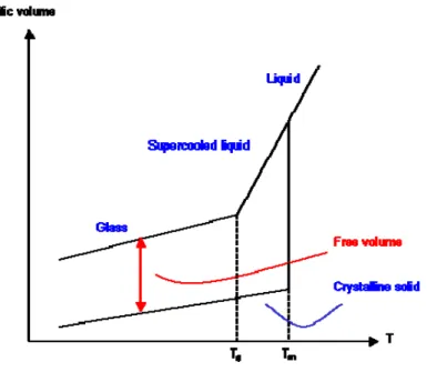
The nature of the glass transition is still the subject of discussions. Though it exhibits features of a second order transition, there is still disagreement whether it is purely kinetic or if it is a kinetic manifestation of an underlying thermodynamic transition [1.33]. However, when a liquid is cooled to form a glassy solid, it transforms from an equilibrium state (liquid) to a non equilibrium state (glass), and its appearance, i.e., the glass transition temperature Tg, is dependent on the rate or time scale of the experiment (see Figure 1.3), contradicting the definition of thermodynamic phase transitions. A way to determine the glass transition temperature Tg is provided by differential scanning calorimetry (DSC). Here, the heat flow of the sample to a reference is monitored and at the glass transition temperature Tg a step is observed that is caused by the discontinuity of the heat capacity Cp.
CHAPTER I - Membrane for gas separation
Figure 1. 3 -Schematic diagram of volume definitions in polymers and temperature dependencies.
Above the glass transition temperature, glass forming amorphous polymers are in a liquid-like or rubbery state. At these temperatures, the enhanced molecular motion permits assemblies of polymer chain-segments to move in a coordinated manner, and hence allowing the material to flow [1.35] the degree of cooperative movement depending on temperature and molecular weight. The enhanced molecular mobility mutually depends on the presence of free volume which provides the space that is required for the rearrangement of the polymer segments to take place.
With decreasing temperature, the mobility of the polymer segments decreases and hence the specific volume Vsp of the polymer decreases according to the thermal expansion coefficient of the liquid state γl, see Figure 1.3. At the glass transition temperature, long range
cooperative movement of polymer segments ceases, and while short-ranged rearrangements of individual mobile units of the polymer chain may still be possible, the restricted coordinated movement of the entangled macromolecular chains below the glass transition temperature turns the polymer into a solid glass, preserving the amorphous structure of the liquid or rubbery state.
Volume changes now follow the thermal expansion coefficient of the solid γs. The
transition temperature Tg depends on the rate of cooling, as does the amount of frozen-in free volume. At slower rates, the glass transition temperature decreases and less free volume is conserved. Starting from the specific volume of the polymer Vsp different occupied volumes
may be subtracted to give a measure of the free volume:
i) Vsp − VvdW, the van der Waals volume of the polymer chains, gives the free volume at 0
K.
ii) Vsp − Vc, the volume of a hypothetical, close packed crystal, gives the excess free
CHAPTER I - Membrane for gas separation
iii) Vsp −Vl, the extrapolated volume of an undercooled liquid, gives the amount of
unrelaxed free volume.
Commonly glassy polymers are characterized with respect to the free volume by calculation of the fractional free volume using the method of Bondi [1.33]:
sp vdW sp free FV V V V V 3 . 1 1 (1.18)
CHAPTER I - Membrane for gas separation
REFERENCES
[1.1] P. Bernardo, E. Drioli, G. Golemme, Ind. Eng. Chem. Res. 48 (2009) 4638. [1.2] F. M. Dautzenberg, M. Mukherjee Chem. Eng. Sci. 56 (2001) 251.
[1.3] W. J. Koros, Editorial. Three hundred volumes. J. Membr. Sci. 300 (2007) 1. [1.4] R. W. Baker, Ind. Eng. Chem. Res. 41 (2002) 1393.
[1.5] H. Strathmann, . AIChE J., 47 (2001) 1077. [1.6] L. M. Robeson, J. Membr. Sci. 62 (1991) 165. [1.7] B. D. Freeman, Macromolecules 32 (1999) 375.
[1.8] H. Strathmann, L. Giorno, E. Drioli, An introduction to membrane science and technology, Publisher CNR, Roma, ISBN 88-8080-063-9, 2006
[1.9] B.D. Freeman, I. Pinnau, Polymeric materials for gas separation, in: B.D. Freeman, I. Pinnau (Eds.), Polymer Membranes for Gas and Vapor Separation, ACS Symposium Series 733, American Chemical Society, Washington, DC, 1999, p.1.
[1.10] W.J. Koros and G.K. Fleming, J. Membr. Sci., 83 (1993) 180.
[1.11] R. W. Baker Gas separation. In Membrane Technology and Applications, 2nd ed.; John Wiley: Chichester UK, 2004; pp 287-335.
[1.12] L.M. Robeson, J.Membrane Sci., 320 (2008) 390.
[1.13] L.M. Robeson, W.F. Burgoyne, M. Langsam, A.C. Savoca, C.F. Tien, Polymer 35 (1994) 4970.
[1.14] K.K. Hsu, S.Nataraj, R.M. Thorogood, P.S. Puri, J. Membr. Sci. 79 (1993) 1.
[1.15] J. Won, M.H. Kim, Y.S. Kang, H.C. Park, U.Y. Kim, S.C. Choi, S.K. Koh, J. Appl. Polym. Sci. 75 (2000) 1554.
[1.16] J.D. LeRoux, D.R. Paul, J. Kampa, R.J. Lagow, J. Membr. Sci. 94 (1994) 121. [1.17] J.D. LeRoux, V.V. Teplyakov, D.R. Paul, J. Membr. Sci. 90 (1994) 55.
[1.18] C.M. Zimmerman, A. Singh, W.J. Koros, J. Membr. Sci. 137 (1997) 145. [1.19] S. Husain,W.J. Koros, J. Membr. Sci. 288 (2007) 195.
[1.20] T.-S. Chung, L.Y. Jiang, Y. Li, S. Kulprathipanja, Prog. Polym. Sci. 32 (2007) 483. [1.21] D. Sen, H. Kalipcilar, L. Yilmaz, J. Membr. Sci. 303 (2007) 194.
[1.22] C.W. Jones, W.J. Koros, Carbon 32 (1994) 1419.
[1.23] Y.K. Kim, H.B. Park, Y.M. Lee, J. Membr. Sci. 255 (2005) 265.
[1.24] H.B. Park, C.H. Jung, Y.M. Lee, A.J. Hill, S.J. Pas, S.T. Mudie, E. Van Wagner, B.D. Freeman, D.J. Cookson, Polymers with cavities tuned for fast selective transport of small molecules and ions, Science 318 (2007) 254.
[1.25] Y. Yampolskii, Russian Chemical Reviews, 2007, 76, 59-78 Chapter 2: Perfluoropolymer membranes and free volume in polymers
[1.26] A. Y. Alentiev, Y. Yampolskii, V. P. Shantarovich, S. M. Nemser, N. A. Platè, J. Memb. Sci., 126 (1997) 123.
[1.27] A. Y. Alentiev, Y. Yampolskii, J. Memb. Sci., 165 (2000) 201. [1.28] M. H. Cohen, D. Turnbull, J.Chem. Phys, 31 (1959) 1164. [1.29] D. Turnbull, .M. H. Cohen, J.Chem. Phys, 34 (1961) 120.
[1.30] J. S. Vrentas, J. L. Duda, in Encyclopedia of Polymer Science and Engineering, New York, Wiley 1986.
CHAPTER I - Membrane for gas separation
[1.31] J. L. Duda, J. M. Zelinsky, Free-Volume Theory in Diffusion in Polymers, New York, Marcel Decker, 1996.
[1.32] A. Bondi, Physical properties of Molecular Crystals, Liquids and Gases, N.Y., Wiley, 1968.
[1.33] G. B. McKenna and S. L. Simon. The Glass Transition: Its Measurement and Underlying Physics. In S. Z. D. Cheng, editor, Applications to Polymers and Plastics, volume 3 of Handbook of Thermal Analysis and Calorimetry, book chapter 2. Elsevier Science B.V., 2002.
[1.34] P. Ehrenfest. Phase Proceedings of the Koninklke Akademie Van Wetenschappen Te Amsterdam, 36 (1933) 153.
[1.35] L. H. Sperling. Introduction to Physical Polymer Science. Wiley-Interscience, New York,2001.
CHAPTER II – Theoretical Basis of Molecular Simulation
II. THEORETICAL BASIS OF MOLECULAR SIMULATION
1. Introduction
The main goal of computational materials science is the rapid and accurate prediction of properties of new materials before their development and production. In order to develop new materials and compositions with designed new properties, it is essential that these properties can be predicted before preparation, processing, and characterization.
Polymers are complex macromolecules whose structure varies from the atomistic level of the individual backbone bond of a single chain to the scale of the radius of gyration, which can reach tens of nanometers. Polymeric structures in melts, blends and solutions can range from nanometer scales to microns, millimeters and larger. The corresponding time scales of the dynamic processes relevant for different materials properties span an even wider range, from femtoseconds to milliseconds, seconds or even hours in glassy materials, or for large scale ordering processes such as phase separation in blends.
Molecular modeling and simulation combines methods that cover a range of size scales in order to study material systems [2.1].
These range from the sub-atomic scales of quantum mechanics (QM), to the atomistic level of molecular mechanics (MM), molecular dynamics (MD) and Monte Carlo (MC) methods, to the micrometer focus of mesoscale modeling.
Quantum mechanical methods have undergone enormous advances in the past 10 years, enabling simulation of systems containing several hundred atoms. Molecular mechanics is a faster and more approximate method for computing the structure and behaviour of molecules or materials. It is based on a series of assumptions that greatly simplify chemistry, e.g., atoms and the bonds that connect them behave like balls and springs. The approximations make the study of larger molecular systems feasible, or the study of smaller systems, still not possible with QM methods, very fast. Using MM force fields to describe molecular-level interactions, MD and MC methods afford the prediction of thermodynamic and dynamic properties based on the principles of equilibrium and non-equilibrium statistical mechanics [2.2-2.6] Mesoscale modeling uses a basic unit just above the molecular scale, and is particularly useful for studying the behaviour of polymers and soft materials. It can model even larger molecular systems, but with the commensurate trade-off in accuracy [2.7-2.9]. Furthermore, it is possible to transfer the simulated mesoscopic structure to finite elements modeling tools for calculating macroscopic properties for the systems of interest [2.10].
CHAPTER II – Theoretical Basis of Molecular Simulation
Figure 2. 1 – Multiscale molecular modeling: characteristic times and distances.
There are many levels at which modeling can be useful, ranging from the highly detailed ab initio quantum mechanics, through classical molecular modeling to process engineering modeling. These computations significantly reduce wasted experiments, allow products and processes to be optimized, and permit large numbers of candidate materials to be screened prior to production.
Over the last 20 years detailed atomistic molecular modeling techniques based on classical molecular mechanics have become a widely used method for the investigation of the molecular structure of membrane materials for gases separation based on amorphous polymers and the sorption and diffusion of low molecular weight penetrants in these materials [2.11]. The interest in development and application of molecular dynamics methodologies for the investigation of micro-structure of polymeric materials for gas separation is due to the fact that on the one hand major aspects of the small molecule membrane separation mechanisms are determined by the static structure on an atomistic scale and the dynamic behavior on a timescale ranging from picoseconds (ps) to nanoseconds (ns) of the separation system (membrane plus penetrants); it is impossible to get any direct experimental data about what is happening in these dimensions during the separation process.
To rectify this situation, better theoretical understanding of the transport mechanism and of the main factors which determine the permeability and permselectivity of dense amorphous polymers on a molecular level is clearly required. Furthermore, quantitative predictions of
CHAPTER II – Theoretical Basis of Molecular Simulation
separation properties on the basis of the monomer composition of amorphous polymers would be very useful.
2. Force Field Based Simulation
The interaction of particles, bonded or nonbonded, is subject to a quantum mechanical description. In principle, for the physically most accurate description available, the Schrödinger-equation for each particle (electrons and nuclei) must be devised, leading to a complex set of equations. Its solution is, though possible, beyond reasonable effort for the size of the systems and the CPU-power available. However, the properties which are under investigation in this work, i.e., static, thermodynamic and dynamic (transport and relaxational) properties of non-reactive organic polymers, are well described using forcefield based molecular mechanics (MM), molecular dynamics (MD) and classical Monte Carlo (MC) simulations [2.12, 2.13] methods based on classical mechanics of multi-particle systems. Needless to say, some quantum mechanical information and experimental data are needed to establish the forcefield in the first place.
The information is obtained for relatively small units and is, by extrapolation, assumed to be valid for larger systems of equal classes.
2.1. The ForceField
Forcefields allow the calculation of the potential energy U of an ensemble of N atoms, as a function of their coordinates (r1 . . . rN). It is composed of individual contributions which
describe the interactions of bonded atoms (bond-lengths, -angles, conformation angles) and nonbonded interactions (van der Waals, electrostatic):
(2.1) The contributions of bonded interactions are represented by anharmonic oscillators of the form [2.14]:
CHAPTER II – Theoretical Basis of Molecular Simulation
0
4 3 3 0 2 2 0 1 ) ( ij ij ij ij ij ij ij ij r k r r k r r k r r U (stretch)
0
4 3 3 0 2 2 0 1 )( ijk ijk ijk ijk ijk ijk ijk
ijk k k k U (angle)
0
4 3 3 3 0 2 2 2 0 111 cos 1 cos 1 cos
)
(il il il il
ijkl k k k
U (torsion)
(2.2) The force constants ki and the equilibrium positions rij , θijk and Φi−l are based on results of
quantum mechanics and constitute the integral part of the forcefield. The nonbonded interactions are expressed in the applied forcefield by a van derWaals term with a 9,6-potential and a coulomb-term:
ij j i ij ij ij ij j i ij ij r q q r B r A q q r U 0 6 9 ) , , ( (nonbonded) (2.3) where Aij and Bij are parameters describing the strength of the repulsive and attractive
force, qi and qj are the partial charges of the interacting atoms and ε0 is the vacuum
permittivity. The forcefield is defined by the functional form (eqns. 2.2, 2.3) and a set of parameters ki, r0ij , . . . which are specific to types of atoms, i.e., account for different bonded
states of the atoms.
For a given molecular structure, the force- field results in a potential energy surface, which can be evaluated with respect to local energy minima. These methods are known as molecular mechanics (MM) [2.14]. In the course of optimization, geometrically reasonable (static) structures can be obtained from the initially guessed geometry by varying the atom positions and minimizing the potential energy of the system.
It should be noticed that the evaluation of the nonbonded energy terms is the numerically most extensive part in molecular modeling calculations because these terms include contributions from each pair of atoms in a model. This leads to restrictions on the maximum possible size of a simulated membrane system (e. g. an amorphous polymer packing). The number of atoms N can not be much higher than 2000–10000 for typical transport simulations on modern workstations, while N may be up to about a factor of ten higher for selected simulations on currently available supercomputers.
2.2. Molecular dynamics (MD)
To perform molecular dynamics (MD) simulations, the forces that result from the forcefield and which act on each atom are applied to the system of finite temperature, i.e., finite kinetic energy Ekin.
Each of the N particles is assigned a random (Boltzmann) velocity vector r’i so that the
CHAPTER II – Theoretical Basis of Molecular Simulation
N
k T r m E n i i B i kin 2 6 3 2 1 2 1
(2.4)Here (3N −6) is the number of degrees of freedom and kB is the Boltzmann constant. in
the course of a simulation, integration of the Newtonian equations of motion:
i i N i ri i U r r mr F ( 1,..., ) (2.5)
leads to a new velocity of each particle which can be extrapolated over the time step Δt = 1 fs of the simulation to determine the new coordinates ri. The force Fi, acting on a particle i
of mass mi, results from the gradient of the potential energy Ui (see eq. 2.4) determined by the
forcefield (eq. 2.1.)
Using Eq. (2.3-4) it is then possible to follow the motions of the atoms of a polymer matrix and the diffusive movement of imbedded small penetrant molecules at a given temperature over a certain interval of time. Eq. (2.4) represents a system of usually several thousand coupled differential equations of second order. It can be solved only numerically in small timesteps Δt [2.15-2.17]. The choice of the time step Δt results from the consideration that the fastest vibration of the system should be sufficiently resolved. In a typical IR-spectrum, the C-H-bond shows a characteristic peak at υ(C-H) ≈ 3000 cm−1, which corresponds to an oscillation period of τ (C-H ) ≈10fs.
3. Condensed Phase Simulation
When simulating condensed-phase systems, it is necessary to build systems that can present the bulk of the simulated materials correctly. Therefore the size of the simulation cell must be large enough to be able to sample the configurational space of the properties of interested. On the other hand, the system size is also limited by computing power (about 10,000 atoms for molecular dynamics).
3.1. Periodic Boundary Conditions
When taking a small system out of the bulk of simulated object, the same bulky environment has to be preserved to avoid unrealistic surface effect. The common approach is to use the periodic boundary conditions, in which the primary cell (parent cell) is surrounded on all sides by replica of itself (image cells) to form a three-dimensional infinite lattice. The atoms initially in the parent cell are parent atoms, while those initially in the image cells are image atoms. There is an image centering technique to control the constant atom number, i.e. whenever an atom migrates to the edge of the primary cell, it will appear in the adjacent image cell.
However, its image will enter the primary cell on the opposite side. Thus atoms may diffuse as far as they can during the course of the simulation instead of being confined in the small parent cell, and at the same time the number of atoms in the box is always constant. In an explicit image model a parent atom will interact with any image atoms (besides parent atoms) within the user-defined cutoff while implicit image model only counts the closest image atoms [2.18].
CHAPTER II – Theoretical Basis of Molecular Simulation
3.2. Amorphous Cell Construction
Polymer chain can adopt numerous conformations due to the existence of many rotatable bonds, whereas for small molecules, only limited number of conformations are accessible. Even a short polymer chain may have a few hundred rotatable bonds that give rise to millions of different conformers. This makes it difficult to sample all the conformations of a real polymer chain with a small simulation cell. It is almost impossible to find the “global” minimum energy conformation within such a large configuration space using energy minimization scheme. Also it is very time consuming if not impossible to equilibrate polymers with unrealistic initial structure by molecular dynamics. The interdependent RIS (Rotational Isomeric State) model has been proved to be an efficient and effective way to build a polymer chain of reasonable initial structure since condensed-phase polymer chain is known to be at unperturbed state. However, the conventional pair wise RIS model does not explicitly prohibit overlapping of atoms separated by a few backbone atoms away or atoms belonging to different molecules.
A method developed by Theodorou and Suter [2.19] takes advantage of the conventional RIS model while overcomes such limitations. In their method, a Monte Carlo type bond-by-bond construction scheme is employed to build a polymer backbone.
Usually amorphous cells are built at a relatively low initial density with ease and are compressed to the experimental density gradually using high-pressure NPT dynamics.
These cells generally need to be further refined to “equilibrate” the structure. The refinement adopted in present studies is an annealing procedure, which will heat up polymer cell step by step using high temperature NPT molecular dynamics, then cool it back to the original conditions. This procedure is particular useful for rubbery polymers that have a flexible backbone. High temperature dynamics may provide sufficient amount of energy for the polymer chains to overcome local energy barriers and reach “global” minimum energy conformation.
3.3. The Concept of Ensembles
In statistical thermodynamics, details of individual particles are usually not of great importance. On the contrary, for a realistic representation of thermodynamic behaviour, the expectancy of observable properties are regarded. This may be achieved by taking the mean value with respect to time or as the average of a number of configurations.
In molecular dynamics, the evolution of a system with respect to time is observed. Depending on the property under investigation, different ensembles are evaluated, i.e., different state-variables are held constant to observe the behaviour of others.
In the microcanonical ensemble the number of particles N, the total energy E and the volume of the simulation cell V are held constant. While keeping N and E constant is quite straightforward and needs no further explanation, the volume V of a system may be kept constant by periodic boundary conditions (see 3.1), forcing a particle that leaves the virtual simulation cell to enter on the opposite side by assigning the appropriate coordinates.
CHAPTER II – Theoretical Basis of Molecular Simulation
A canonical ensemble is characterized by constant N, V and temperature T. The easiest way to control the temperature is to directly scale the particle velocities ri, whenever the
system temperature Tsys leaves a predefined temperature window T0 ± ΔT:
2 1 0 , , sys old i now i T T r r (2.6)
More refined methods like the Berendsen thermostat [2.20] are more commonly used because a temperature change per simulation time step leads to a more smooth progression of the temperature. In this work, molecular dynamics are applied to canonical ensembles as part of the equilibration steps in the packing procedure (see Chapter 3 section 1.3). and referred to as NVT -MD (according to the state variables N, V and T that are kept constant).
If, at constant N and T, the pressure p is held constant instead of the volume V the ensemble is called isothermal-isobaric. The pressure is evaluated using the virial Ξ and kinetic energy Ekin NkBT based on centers of mass [2.20]:
j i ij ij t F t r t ( ) ( ) 2 1 ) ( (2.7)It is controlled by changing the volume V of the simulation cell according to the relation: 3 2 T Nk pV B (2.8)
Molecular dynamics simulations of isothermal-isobaric ensembles (NpT -MD) are performed as final equilibration procedure of the packing models (see Chapter 3 section 1.3).
An ensemble of constant pressure, volume, temperature and chemical potential μ is called grand canonical. Here, the number of particles N is allowed to fluctuate. This is achieved by randomly inserting or deleting molecules. The chemical potential of the molecules within the matrix is balanced with a reference chemical potential, e.g. that of a surrounding gas phase at corresponding pressure and temperature. Using a Monte Carlo algorithm, a new configuration is energetically evaluated and accepted if more favourable than the previous and otherwise rejected, allowing for thermal fluctuations using a temperature dependent Boltzmann factor. Grand Canonical Monte Carlo (GCMC) simulations are used in this work to calculate sorption equilibrium on static packing models for several pressures (chemical potentials) at constant volume and temperature to determine concentration-pressure isotherms which are referred to as GCMC-isotherms (see Section 4.3.1).
4. Simulation of gas transport properties
4.1. Calculation of diffusion coefficients
CHAPTER II – Theoretical Basis of Molecular Simulation
i
i D a
J (2. 9)
where Ji denotes the flux of particles of species i and ai is its activity (usually we assume the
activity equals the concentration). Fick’s law holds in the case of thermal and mechanical equilibrium (constant T and p).
From the microscopic point of view, the diffusion coefficient can be related to the autocorrelation function of particle velocity:
i i i i i v t dt v D (0) ( ) 3 1 (2.10)if the diffusion species concentration is low and the interaction between these particles is a short-range interaction, Equation 2.9 can be simplified to
i vi t vi dt D ( ) (0) 3 1 (2.11)which is know as the Green-Kubo relation for the diffusion coefficient.
This equation states that the diffusivity is given by the time integral of the single particle center-of-mass velocity autocorrelation function. Under the long-time condition, Equation 2.8 was shown to be equivalent to the Einstein equation:
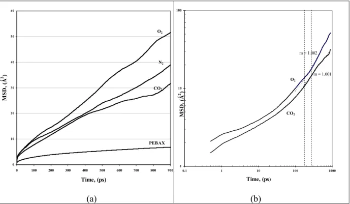
2 ) 0 ( ) ( lim 6 1 i i t t N D r r (2.12)
Where N is the number of diffusing molecules of type α, ) ri(0 and )ri(t are the initial and final positions of molecules (mass centres of particle i) over the time interval t, and
2 ) 0 ( ) ( i i t r
r is the mean square displacement (MSD) averaged over the possible ensemble. The Einstein relationship assumes a random-walk motion for the diffusing particles [2.22].
In this case, Dα is linearly proportional to the MSD. For slow diffusing species, anomalous diffusion is sometime observed and characterized by:
n i i t t 2 ) 0 ( ) ( r r (2.13)
where n < 1 (for Einstein diffusion regime, n = 1). At short dynamics time range, the MSD may be quadratic to time (i.e. n = 2), this represents the occurrence of free flight of diffusing species. At sufficient long time (i.e. hydrodynamic limit), a transition from anomalous to Einstein diffusion (n =1) may be observed.
The resulted diffusion coefficient (Dα) is often called the tracer diffusion coefficient or the self-diffusion coefficient. It’s a dynamic property under equilibrium state. While the diffusivities obtained from experiments ( Dij ) are often referred as transport coefficients. The
relationship of these two diffusion coefficients in a two components (A, B) system is often expressed by Darken’s equation [2.23, 2.24]: