Synthesis of Metamaterial-Enhanced Radiating Devices

(1)

UNIVERSITY

OF TRENTO

DIPARTIMENTO DI INGEGNERIA E SCIENZA DELL’INFORMAZIONE

38123 Povo – Trento (Italy), Via Sommarive 14

http://www.disi.unitn.it

SYNTHESIS OF METAMATERIAL-ENHANCED RADIATING

DEVICES

E. T. Bekele, F. Viani, L. Manica, and Douglas H. Werner

October 2012

(2)

(3)

1 Introduction

This report presents description of the qTO software package. The application of the software is demonstrated with an example test case provided with the software. An additional test case considering theoretical Transformation Electromag-netics is also reported.

(5)

2 Description of the qTO software

The software package implements a quasi-conformal transformation (qTO) in two dimensions. In its canonical applica-tion, polygons in virtual plane are transformed to rectangular regions in the physical plane. The polygon in the virtual plane is expected to have a constant material properties (εr,µr) and the software computes the material properties in the

rectangular region that can support equivalent electromagnetic properties. The reverse transformation from a rectangle in virtual plane to polygon in physical plane is also supported but material properties are not computed in this case.

The software is organized as a package qTO and the core of the software is the class Transformation. This class contains routines (methods) to perform “normal” and inverse transformations. The normal transformation is implemented by the function Transformation.build(path,cornerpoints,gridx,varargin). The argument path defines the (x, y) coordinates of the boundary of the virtual polygon. In the construction of the shape, consecutive points in path are joined by straight line, therefore curved regions need to be sampled more densely. A grid is generated(How?) in the virtual and physical planes, and the software requires four(Why four? Which four?) corners of the polygon as input for grid generation. The argument cornerpoints defines these corners. The inverse mapping is implemented in the function T.Inverse(). In addition, the package contains extensive tools for graphical output.

(6)

3 Example 1: Double Convex Lens

This example is included with the software as a demonstration. The example includes design of a Transformation Optics (TO) flat biconvex lens extended with a box (in the sense of optical focusing).

3.1 Virtual Object parameters:

The classical constant refractive index (constant εrand µr) lens (in the virtual plane) has the following parameters:

• Radius of curvature: r = 50 (arbitrary units) • Lens Width: w = 30(arbitrary units)

• Lens thickness at corner: t = 5 (arbitrary units) • Lens angle: thb = 150

• Relative permittivity: εr= 4

• Non-magnetic lens: µr= 1

3.2 Result and Discussion

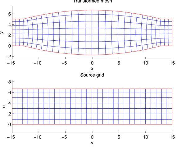
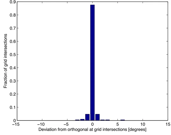
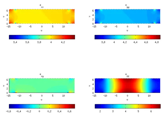
The result of the transformation is described as follows. Figure 1 shows geometries and grids in virtual(top) and phys-ical(bottom) plane. It is stated that quasi conformal mapping perturbs orthogonality of the grid(How?). This means accuracy of isotropic medium approximation is reduced(How?). It is also stated that this effect is small and can be ne-glected. Additional figures are provided to demonstrate that the effect of the perturbation is “small” and can be nene-glected. Towards this end, Figure 4 shows the fraction of grid intersections that deviate from orthogonality. It can be seen that very few fraction of entries deviate from orthogonality. Figure 5 shows the actual material properties, with no isotropic approximation. The off-diagonal entries in this figure (exy) are approximately zero nearly throughout the rectangle, hence

can be “reasonably” approximated to be constant zero. Values for exxand eyyare nearly constant throughout the region

(7)

−15 −10 −5 0 5 10 15 −2 0 2 4 6 x y Transformed mesh −15 −10 −5 0 5 10 15 0 2 4 6 8 v u Source grid

Figure 1: qTO transformation of biconvex lens: Transformed(virtual plane) and Source(physical plane) grids.

−15 −10 −5 0 5 10 −6 −4 −2 0 2 4 6 8 10 12 u

Isotropic transformation permittivity ( !_zz ) gradient

v

2 2.5 3 3.5 4 4.5 5 5.5 6 6.5

(8)

2.5 2.5 2.25 2.25 2 2 1.75 1.75 2.5 2.5 2.25 2.25 2 2 1.75 1.75 −15 −10 −5 0 5 10 15 −6 −4 −2 0 2 4 6 8 10 12 u v

Isotropic transformation index ( n ) gradient

1.75 1.75 2 2 2.25 2.25 _2.5 2.5 1.8 1.9 2 2.1 2.2 2.3 2.4 2.5

Figure 3: qTO transformation of biconvex lens: Isotropic transformation Refractive index, (n), gradient in the physical plane.

−150 −10 −5 0 5 10 15 0.1 0.2 0.3 0.4 0.5 0.6 0.7 0.8 0.9

Fraction of grid intersections

Deviation from orthogonal at grid intersections [degrees]

(9)

(10)

4 Example 2: Field Concentrator

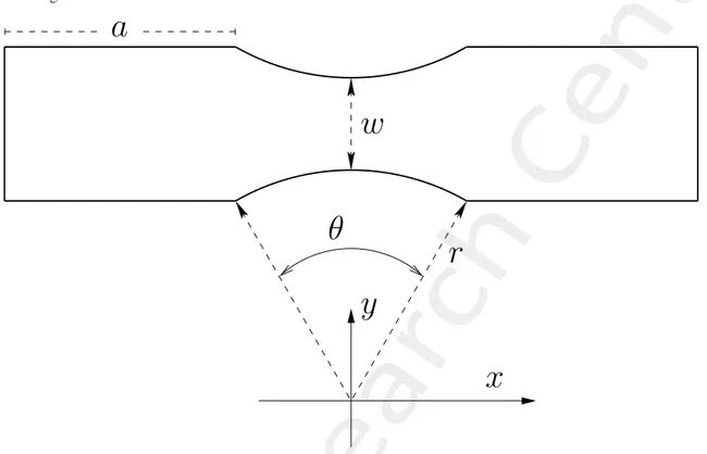
To demonstrate use of the software package in the context of transformation electromagnetics (TE), an example different from the one provided with the software is considered. Here a synthesis of theoretical field concentrator is attempted based on the a simple coordinate transformation example provided in [1]. In the virtual plane, the propagation medium is constricted at its center and the wave is forced to traverse this narrow region. The geometry of the proposed virtual object is shown in Figure 6.

y

x

r

w

a

θ

Figure 6: qTO transformation of field concentrator: Geometry of proposed virtual structure.

4.1 Virtual Object parameters:

With reference to the labels in Figure 6, the virtual object is parametrized as follows: • Radius : r = 50 (arbitrary units)

• w = 20(arbitrary units) • a = 50 (arbitrary units) • Arc angle: θ = 600

• Constant relative permittivity: εr= 4

• Non-magnetic medium: µr= 1

4.2 Result and Discussion

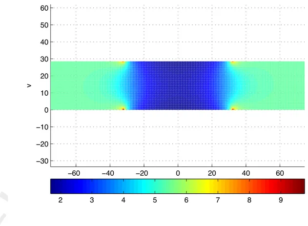
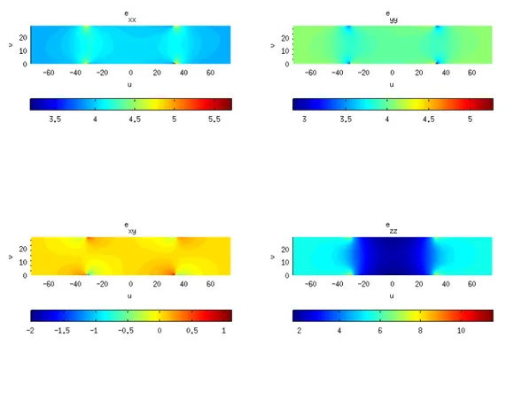
The transformation was peformed mimicking the previous example, and the result of the transformation are presented as follows. Figure 7 shows the transformation grid in both physical and virtual planes. Figure 8 reports medium permittivity for with isotropic approximation. The gradient of the refractive index is reported in Figure 9. When compared to the previous example (Figure 4 vs Figure 10), one can see that the fraction of non-orthogonal grid crossings has increased. The exact (anisotropic) medium parameters are reported in Figure 11. Also in this case, exy component of the relative

permittivity tensor has near zero values throughout most the region of interest. Similarly, the components exxand eyyare

(11)

−60 −40 −20 0 20 40 60 40 50 60 70 80 x y Transformed mesh −60 −40 −20 0 20 40 60 −10 0 10 20 30 v u Source grid

Figure 7: qTO transformation of field concentrator: Transformed(virtual plane) and Source(physical plane) grids.

−60 −40 −20 0 20 40 60 −30 −20 −10 0 10 20 30 40 50 60 u

Isotropic transformation permittivity ( !_zz ) gradient

v

2 3 4 5 6 7 8 9

(12)

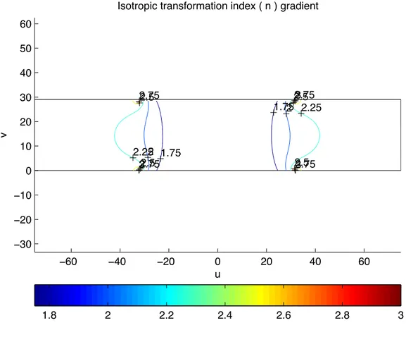
3 3 3 2.75 2.75 2.75 2.75 2.5 2.5 2.5 2.5 2.25 2.25 2 2 1.75 1.75 3 3 3 2.75 2.75 2.75 2.75 2.5 2.5 2.5 2.5 2.25 2.25 2 2 1.75 1.75 −60 −40 −20 0 20 40 60 −30 −20 −10 0 10 20 30 40 50 60 u v

Isotropic transformation index ( n ) gradient

1.75 1.75 2 2 2.25 2.25 2.5 2.5 2.5 2.5 2.75 2.75 2.75 2.75 3 3 3 1.8 2 2.2 2.4 2.6 2.8 3

Figure 9: qTO transformation of field concentrator: Isotropic transformation Refractive index, (n), gradient in the physical plane.

−150 −10 −5 0 5 10 15 0.1 0.2 0.3 0.4 0.5 0.6 0.7

Fraction of grid intersections

Deviation from orthogonal at grid intersections [degrees]

(13)

(14)

Acknowledgment

This work is supported by Autonomous Province of Trento - Call for proposal “Team 2011”.

References

[1] D.-H. Kwon and D. H. Werner, “Transformation electromagnetics: An overview of the theory and applications,”

IEEE Antennas Propag. Mag., vol. 52, no. 1, pp. 24-26, Feb. 2010.

[2] P. Rocca, M. Benedetti, M. Donelli, D. Franceschini, and A. Massa, ”Evolutionary optimization as applied to inverse problems,” Inverse Problems - 25th Year Special Issue of Inverse Problems, Invited Topical Review, vol. 25, pp. 1-41, Dec. 2009.

[3] P. Rocca, G. Oliveri, and A. Massa, ”Differential Evolution as applied to electromagnetics,” IEEE Antennas and Propagation Magazine, vol. 53, no. 1, pp. 38-49, Feb. 2011.

[4] G. Oliveri and A. Massa, ”GA-Enhanced ADS-based approach for array thinning,” IET Microwaves, Antennas & Propagation , vol. 5, no. 3, pp. 305-315, 2011.

[5] G. Oliveri, F. Caramanica, and A. Massa, ”Hybrid ADS-based techniques for radio astronomy array design,” IEEE Transactions on Antennas and Propagation - Special Issue on ”Antennas for Next Generation Radio Telescopes,” vol. 59, no. 6, pp. 1817-1827, Jun. 2011.

[6] L. Poli, P. Rocca, G. Oliveri, and A. Massa, ”Harmonic beamforming in time-modulated linear arrays,” IEEE Trans-actions on Antennas and Propagation, vol. 59, no. 7, pp. 2538-2545, Jul. 2011.

[7] L. Poli, P. Rocca, L. Manica, and A. Massa, ”Handling sideband radiations in time-modulated arrays through particle swarm optimization,” IEEE Transactions on Antennas and Propagation, vol. 58, no. 4, pp. 1408-1411, Apr. 2010. [8] L. Poli, P. Rocca, L. Manica, and A. Massa, ”Time modulated planar arrays - Analysis and optimization of the

sideband radiations,” IET Microwaves, Antennas & Propagation, vol. 4, no. 9, pp. 1165-1171, 2010.

[9] L. Lizzi, F. Viani, R. Azaro, and A. Massa, ”Optimization of a spline-shaped UWB antenna by PSO,” IEEE Antennas and Wireless Propagation Letters, vol. 6, pp. 182-185, 2007.

[10] L. Lizzi, F. Viani, R. Azaro, and A. Massa, ”A PSO-driven spline-based shaping approach for ultra-wideband (UWB) antenna synthesis,” IEEE Transactions on Antennas and Propagation, vol. 56, no. 8, pp. 2613-2621, Aug. 2008. [11] P. Rocca, L. Manica, and A. Massa, ”An improved excitation matching method based on an ant colony

optimiza-tion for suboptimal-free clustering in sum-difference compromise synthesis,” IEEE Transacoptimiza-tions on Antennas and Propagation, vol. 57, no. 8, pp. 2297-2306, Aug. 2009.

[12] P. Rocca, L. Manica, and A. Massa, ”Ant colony based hybrid approach for optimal compromise sum-difference patterns synthesis,” Microwave and Optical Technology Letters, vol. 52, no. 1, pp. 128-132, Jan. 2010.

[13] P. Rocca, L. Manica, F. Stringari, and A. Massa, ”Ant colony optimization for tree-searching based synthesis of monopulse array antenna,” Electronics Letters, vol. 44, no. 13, pp. 783-785, Jun. 19, 2008.

[14] G. Oliveri and L. Poli, ”Optimal sub-arraying of compromise planar arrays through an innovative ACO-weighted procedure,” Progress in Electromagnetic Research, vol. 109, pp. 279-299, 2010.

[15] G. Oliveri, ”Improving the reliability of frequency domain simulators in the presence of homogeneous metamaterials â A preliminary numerical assessment,” Progress In Electromagnetics Research, vol. 122, pp. 497-518, 2012.