Author: Maria Armengol i D´ıaz
Facultat de F´ısica, Universitat de Barcelona, Diagonal 645, 08028 Barcelona, Spain.
Advisor: Ana Maria Vila i Arbones
Abstract: In this project we study two circuits that allow us to create a simple Theremin, one of them based on analog components and the other one on digital devices. First, we design the circuits and study them analytically, checking that in theory both are valid for our purpose. Then, we simulate them using LTSpice and we observe their behavior. Finally, we try to built them in order to create our own Theremin but we are only successful implementing the analog one.
I. INTRODUCTION
Lev Sergeevich Termen (1896-1993) was a Russian physicist and musician. While he was working at Iofee Physical Technical Institute on high-frequency measure-ment methods he discovered that the movemeasure-ment of ob-jects nearby a circuit affected the capacitance of elec-tronic devices and caused the variation of the resonant frequency. He used that effect to create a musical in-strument that is played without any physical contact between it and the interpreter. Its original name was aetherphone, but it became popular with the name of its creator: Theremin [1].
The Theremin consists of two antennas mounted hor-izontally and vertically respectively. The pitch is con-trolled by the distance between the right hand of the musician and the vertical antenna, being higher with the proximity. The distance between the left hand and the horizontal antenna determines the volume: the musician can lower the volume by approaching his or her hand.
Throughout history, different circuits have been de-signed to implement this instrument. The original design proposed by Lev Termen was based on vacuum valves. Later on, Robert Moog marketed a Theremin based on transistors. Today we can find several designs proposed by professionals from the area as well as for amateur builders. Regardless of the electronics behind the cir-cuit all the designs share the same operating principle - based on the oscillation of a resonant circuit and the principle of heterodynamics - to control the pitch.
In this article we will study analytically two pitch cir-cuits, an analog and a digital one, which could be used to implement a very basic Theremin: from a variation of few picofarads of the capacity of the antenna they achieve an oscillation in audio frequency. This theoretical study will be supported by computer simulations using LTSpice in order to verify our calculations. Finally we will try to implement them to see how changes our previous study by working with real devices.
II. CAPACITANCE OF THE ANTENNA
Before starting the design of the Theremin circuit we must study the antenna capacitance and the influence of
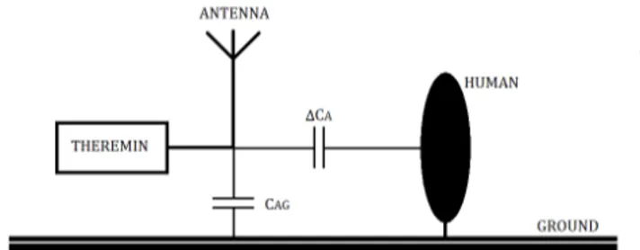
the player. The antenna acts as a plate of a capacitor, creating cylindrical lines of charge in space. Without the presence of a human body, the capacitance CAGbetween the antenna and the ground depends on the electrical, geometrical and location characteristics of the antenna. The hand of the musician acts as a ground plate at a variable distance of the antenna, adding a new capaci-tance ∆CA in parallel (Fig.1) which increases when the performer approach his or her hand [2].
We will use a radio antenna, around 48cm high, to build our Theremin. We experimentally measure its ca-pacitance using a Caca-pacitance Meter model 72B available in our laboratory. Due to the initial offset we can not be able to measure the fixed CAG. We can only measure the variable capacitance ∆CA being 0pF when the musician is far away from the antenna and arround 5pF when he or she almost touches it. As a result of both contributions the antenna capacitance is given by CA= CAG+ ∆CA
Due to the impossibility of measuring CAGwe will use the value of 7pF given in [3] to run our simulations.
FIG. 1: Circuit diagram of capacity antenna model
III. ANALOG THEREMIN DESIGN
To design the Analog Theremin we have based on tra-ditional designs in which two oscillators and a multiplica-tive mixer are used. We use a Wien Bridge as a oscillator, allowing us to study in depth a circuit presented in Elec-tronica Aplicada subject of the degree of Physics. The mixer used is the diode double balanced mixer which al-lows us to work at the desired frequencies. The basic concept is shown schematically in Fig.2
FIG. 2: Block diagram for Analog Theremin
A. Theoretical analysis
The fixed oscillator is a traditional Wien Bridge. Ac-cording to [4] the frequency of oscillation is calculated equaling to zero the imaginary part of the feedback fac-tor, β = V+ Vout, being ff ix= 1 2π√R1R2C1C2 Re[β] = R1 R1(1 +CC12) + R2 (1)
To build a variable oscillator from a Wien Bridge, we locate the antenna in parallel with R3 and C3 as we see in Fig.3. Therefore, we must add a new variable capacity CAin (1), obtaining this new expression:
fvar= 1 2πpR3R4C4(C3+ CA) Re[β] = R3 R3(1 +C3C+CA 4 ) + R4 (2)
As we see in (2) the frequency decreases with CA. In-creasing the value of this variable capacity - by approach-ing the hand - fvar is more different from ff ix
A mixer is a device that creates new frequencies by combining two input frequencies, using the heterodyn-ing technique. The double balanced mixer uses the non-linear property of the diodes to multiply two signals. The signal of the oscillators can be expressed mathematically as A1cos ω1t and A2cos ω2t. The multiplicative mixer provides an output given by
VM IXER= A1A2
2 [cos (ω1− ω2)t − cos (ω1+ ω2)t] (3) where we have used a standard trigonometric identity to obtain that. Thus the output signal has two fre-quency components. By using a low pass filter, with a cutoff frequency fc = 2πRC1 , we attenuated the sum frequency leaving only the beat frequency as an output of the Theremin. By choosing right values of R and C this output can be an audible signal that varies with the movement of the hand. By approaching the hand ∆CA increases therefore the difference between fvar and ff ix also increases consequently the sound is higher.
B. Simulation
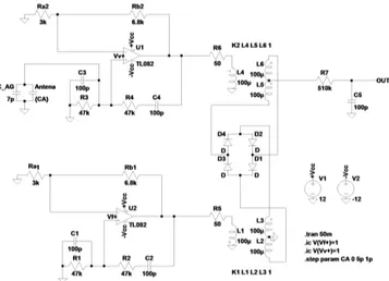
We used the OpAmp TL082 polarized at Vcc= ±12V in order to work with a real device available in the lab-oratory. The selected values of resistance, capacitance and inductance of the components are available in the market.
FIG. 3: Complete Analog Theremin circuit simulation using LTSpice
We choose values of C1,2,3,4 of the order of picofarads, as we can see in Fig.3, so that a minor change of CAwill vary the output some hundreds of Hz. We must note that the closed-loop gain must be Aβ ≥ 1 for all values of CA, otherwise Barkhausen conditions will be broken and the oscillation will be attenuated to zero. Only in the case of equality the output has a sinus shape, in other cases it is saturated near the Vccvoltage.
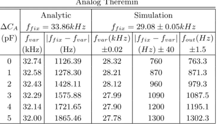
As shown in Table I, simulated values of the resonant frequency are lower than the ones given by (1) and (2), with a relative error of about 13%. By changing the values of R and C we see that we only obtain the exactly theoretical solution by simulating the ideal Wien Bridge, with R1= R2, C1= C2 and Rb= 2Ra, and with values of capacitance around few nanofarads. Despite this, the frecuency variates with ∆CA as expected and the beat frequency |ff ix− fvar| is still in the audio range so we can continue working with this non-ideal circuit.
The mixer’s output have the contributions of the sum and the difference frequency as expected. To filter the signal we choose values of R7 and C5 that cuttoff fre-quencies above 3120Hz to attenuate the sum frefre-quencies. The Output is a sinus wave with ripple - because the attenuation of the sum frequency is not perfect - and this frequency matches perfectly to the difference between simulation values of ff ix and fvar, confirming the ideal operation of the simulated mixer.
Analog Theremin
Analytic Simulation
∆CA ff ix= 33.86kHz ff ix= 29.08 ± 0.05kHz
(pF) fvar |ff ix− fvar| fvar(kHz) |ff ix− fvar| fout(Hz)
(kHz) (Hz) ±0.02 (Hz) ± 40 ±1.5 0 32.74 1126.39 28.32 760 763.3 1 32.58 1278.30 28.21 870 871.3 2 32.43 1428.11 28.12 960 979.3 3 32.29 1575.88 27.99 1090 1087.5 4 32.14 1721.65 27.90 1200 1195.1 5 32.00 1865.46 27.78 1300 1302.3
TABLE I: Analytical and simulation values of frequency of the oscillators signal and the Theremin output of the
Analog Theremin
IV. DIGITAL THEREMIN DESIGN
We design a Digital Theremin using a simplification of the circuit proposed in [3], which uses logic gates as fundamental components. The general idea is the same as the analog circuit: to obtain an audio-frequency sig-nal from the frequency difference between two oscillators. The basic concept is shown schematically in Fig.4.
FIG. 4: Block diagram for Digital Theremin
A. Theoretical analysis
A Schmitt Trigger is a comparator with hysteresis. The gate switches at different points for positive-going and negative-going signal. The threshold voltages are VT + and VT − and the power supply Vdd is referenced to Vss (usually ground). We can use it to built an oscillator as shown in Fig.5. First, Vin is lower than VT + so Vout goes high (Vdd) and starts charging C1,2 through R1,2. When Vin crosses the threshold voltage VT +, Vout goes low (Vss) and discharging of C1,2 through R1,2 begins. When Vin crosses the negative threshold voltage VT −, Vout goes high, hence the process starts again creating an oscillating output which frequency is given by the fol-lowing equation
f = 1
RC lnVT +(V cc−VT −)
VT −(V cc−VT +)
(4)
In the variable oscillator we have the contribution of the capacitance of the antenna, located in parallel with C2, being C = C2+ CA variable and inversely propor-tional to fvar.
The output of the two oscillators is the input of a XOR gate, giving a signal whose duty cycle varies at the differ-ence of the input frequencies. By integrating this signal through a low-pass filter we achieve a pseudo-triangular signal with the beat frequency. Through the well-known Schmitt Trigger gate, we convert this signal into a square wave to eliminate the noise. If we have correctly designed the circuit this signal will be audible and the sound will be higher with the proximity of the hand, similarly to the analog design.
B. Simulation
We polarize all the components of the circuit between Vss= 0V (ground) and Vdd = 5V .
We used simulated 4093B, a two-input NAND gate with VT += 2.9V and VT −= 2.1V , as a Schmitt Trigger. As in the Analog Theremin, we use values of C1,2 of the order of picofarads, obtaining a 5V square signal that varies with CAaccording to (4). In Table II are shown the values of the frequency depending on ∆CA, which mach with the theoretical ones with only 3% of discrepancy.
FIG. 5: Complete Digital Theremin circuit simulation using LTSpice
The XOR must have a quick response time to follow the small variations between ff ix and fvar. We simulate a XOR gate with a response time of 20ns that allows us to obtain the desired signal. Since the difference between the oscillators is at most 1500Hz, we choose the appropri-ate R3and C3to allow pass frequencies of this order and attenuate higher ones. The signal obtained is a sinusoidal wave with ripple. We must ensure that its amplitude is large enough to exceed the VT + and VT − limits of the Schmitt Trigger below. Can be seen in Table II how the final output is in agreement with |ff ix− fvar| besides it is audible and increases with ∆CA.
Digital Theremin
Analytic Simulation
∆CA ff ix= 20.25kHz ff ix= 19.73 ± 0.02kHz
(pF) fvar |ff ix− ff ix| fvar(kHz) |ff ix− fvar| fout(Hz)
(kHz) (Hz) ±0.02 (Hz) ± 40 ±1.5 0 19.35 902.84 18.88 850 860 1 19.22 1025.28 18.76 970 977 2 19.10 1146.19 18.64 1090 1092 3 18.98 1265.58 18.53 1200 1206 4 18.86 1383.50 18.42 1310 1317 5 18.75 1499.95 18.31 1420 1430
TABLE II: Analytical and simulation values of frequency of the oscillators signal and the Theremin
output of the Digital Theremin
V. BUILDING A THEREMIN
During the experimental assembly of the circuits many of the technical problems of this project have emerged. It is also when we have seen the limitations of the dif-ferent components used and we have observed the actual operation of these.
We have used the Power Supply FAC-662B to polarize our circuits, and by means of a TBS 1052B-EDU Digital Oscilloscope we have visualized the output signal of each stage.
A. Analog Theremin
We had technical complications building this circuit, which we will explain below. First we mount the fixed os-cillator successfully obtaining an output of 46.7 ± 0.1kHz - with a relative error of 27% respect the analytic solu-tion that we could attribute to experimental and mea-surement uncertainties-. It is at the time of mounting the variable oscillator when we have a problem. Without con-necting the antenna, the circuit oscillates like the fixed one at 46.7 ± 0.1kHz but when we connect the antenna we see that the oscillation frequency does not change, and by approaching the hand it still does not decreases as we expected. The circuit is not sensitive to the pres-ence of the antenna. We attribute this fact to that the capacitance variation is too small to change significantly the oscillation frequency of the TL082.
B. Digital Theremin
We have been able to successfully build a very simple Theremin from the digital circuit previously studied.
We start with the construction of the oscillators. We use a Schmitt Trigger CD4093B and we verify experi-mentally that VT += 2.9V and VT −= 2.1V . We use the
values of C1,2 and R1,2 indicated in Fig.4 - initially we try to use lower values but thanks to the experimental re-alisation, and according to the Datasheet, we have found that for a correct operation of the oscillating circuit it must be 50kΩ ≤ R ≤ 1M Ω and 100pF ≤ C ≤ 1µF -. Before connecting the antenna in the variable circuit we see that the frequency of the output of the two circuits is slightly different, being 23.0 ± 0.1kHz for the fixed one and 22.5 ± 0.1kHz for the variable, when they should be the same. It is because of working with real compo-nents and not with simulated ones. Both values are suf-ficiently similar (10% of relative error) to the analytical and simulated ones in Table II. Connecting the antenna to the variable circuit causes an immediate decrease of the frequency to 21.4 ± 0.1kHz which, as we have said previously, we attributes to the capacity CAG between the antenna and the ground. Approaching the hand to the antenna we get a signal of 21.0 ± 0.1kHz. Those re-sults are accord to (4), being C = C2+CAG+∆CAwhere CAG = 8 ± 1pF - instead of 7pF as we assumed at the beginning of the work - is fixed and ∆CA= 0 − 4 ± 1pF varies with the movement of the hand.
We introduce the two signals into the XOR 74ls86 ob-taining a periodic signal that, filtered, gives us a signal whose frequency is the difference between them, about 1.6 − 2.1 ± 0.1kHz. We use a third Schmitt Trigger to eliminate the noise and achieve a square wave of 5V of amplitude. This output is in the audio-frequency so we can hear it using a 0.25W ROHS speaker properly con-nected.
(a) VarOsc (blue), FixOsc (yellow)
(b) XOR (blue), LowPassFilter (yellow)
(c) LowPassFilter (yellow), OUT (blue)
FIG. 6: Signal of each block visualized on the oscilloscope
By using a Chromatic tuner CA-30, we verify that the range of notes on the music scale of our Theremin goes from a low G#6 (1661.22Hz) to a C7 (2093.00Hz).
VI. CONCLUSIONS
• We have been able to perform a theoretical study of the operation of two different circuits, understand-ing the physics behind each of their stages and the equations that govern them.
• Through the simulations with LTSpice we have been able to visualize the signal and its dependence with the values of the different components, as well as see how the operation moved away from the ideal analysis.
• Building the experimental setup we have known the limitations of our circuits. We have discarded the analog circuit when we see that it did not work as we expected, attributing this fact to problems of sensibility of the devices. For future work, these experimental problems could be studied in depth in order to solve them and built successfully an Ana-logic Theremin based on Wien Bridges. In contrast, we have been able to develop a very basic Theremin from the digital design studied. This Theremin is purely an academic work, since it allows us to study each of the stages of the circuit, but it can not be considered a musical instrument. Its sound is
un-stable and imprecise, and only supplies a half of an octave therefore is very limited to play music. In addition, the antenna only detects the presence of the hand at a very short distance, so we must work practically by touching the antenna to change the note, which makes the performance very difficult.
• An obvious difference between the two circuits is the form of the output signal, being sinusoidal in the analog one and square in the digital one. This entails a different loudness that we have not been able to hear since we have not been able to build the first circuit.
Acknowledgments
I would like to thank my advisor Ana Maria Vila for the original idea of this work and her guidance during the project. I would also like to thank the department of Enginyeria Electronica for let me access in their lab-oratory and use their equipment throughout the circuit construction phases. Finally I want to thank my family and friends, for their encouragement during all the years of my education.
[1] P. V. Nikitin, “Leon Theremin (Lev Termen)”, IEEE An-tennas and Propagation Magazine 54 (2012) 252-257. [2] W. Buller and W. Brian, “Measurement and Modeling
Mutual Capacitance of Electrical Wiring and Humans”, IEEE Transactions on Instrumentation and Measurement 55 (2006) 1519-1522.
[3] K. D. Skeldon, L. M. Reid, V. McInally, B. Dougan and C. Fulton, “Physics of the Theremin”, American Journal of Physics 66 (1998) 945-955
[4] J. M. Fiore, Amplificadores operacionales y circuitos inte-grados lineales (Delmar Thomson Learning, Madrid, 2001)