A partially unsupervised cascade classifier for the analysis of multitemporal remote-sensing images

UNIVERSITY

OF TRENTO

DEPARTMENT OF INFORMATION AND COMMUNICATION TECHNOLOGY 38050 Povo – Trento (Italy), Via Sommarive 14

http://www.dit.unitn.it

A PARTIALLY UNSUPERVISED CASCADE CLASSIFIER FOR THE ANALYSIS OF MULTITEMPORAL REMOTE-SENSING IMAGES

Lorenzo Bruzzone and Diego Fernández Prieto

2002

Technical Report # DIT-02-0029

A partially unsupervised cascade classifier for the analysis of

multitemporal remote-sensing images

Lorenzo Bruzzone and Diego Fernández Prieto

DICA - University of Trento, Via Mesiano 77, I-38050, Trento, Italy

Telephone: +39-0461-882623; Fax: +39-0461-882672; e-mail: lorenzo.bruzzone@ing.unitn.it

Abstract

A partially unsupervised approach to the classification of multitemporal remote-sensing images is presented. Such an approach allows the automatic classification of a remote-sensing image for which training data are not available, drawing on the information derived from an image acquired in the same area at a previous time. In particular, the proposed technique is based on a cascade classifier approach and on a specific formulation of the expectation-maximization (EM) algorithm used for the unsupervised estimation of the statistical parameters of the image to be classified. The results of experiments carried out on a multitemporal data set confirm the validity of the proposed approach.

Keywords: Multitemporal classification, cascade classifier, unsupervised parameter estimation, remote sensing.

1. Introduction.

In the past few years, there has been a growing interest in the use of remote-sensing systems for a regular monitoring of the earth’s surface. In this context, images acquired on the same area at different times (i.e., multitemporal images) represent a valuable source of information for the observation of the temporal behavior of the land-cover classes that characterize a given region of interest. From an operational point of view, the monitoring

process can be carried out by applying specific supervised classification techniques to the analysis of multitemporal data (Swain, 1978; Kalayeh and Landgrebe, 1986; Khazenie and Crawford, 1990; Jeon and Landgrebe, 1992; Jeon and Landgrebe, 1999; Bruzzone et al., 1999). Unlike standard algorithms for the classification of single-date images, such techniques exploit the temporal correlation between images in order to increase the classification accuracy (a description of these techniques is provided in (Bruzzone et al., 1999)).

A problem arising from the above-mentioned supervised approaches to multitemporal remote-sensing data analysis is that, in general, they require the availability of suitable training data for each image to be categorized. Unfortunately, in most applications, this requirement is not satisfied. In fact, gathering a sufficient number of training samples for each specific image considered, by either photo-interpretation or the collection of “ground truth” information, is very expensive in terms of time and economic cost. Therefore, in many cases, it is not possible to rely on training data for each single image in a multitemporal data set. This prevents the generation of the corresponding land-cover maps by supervised approaches and, consequently, may affect the accurate and efficient monitoring of the considered site.

In this paper, we propose a partially unsupervised approach to the classification of temporal series of multispectral images that overcomes the aforesaid problem. In particular, it allows the automatic classification of a remote-sensing image, for which training data are not available, drawing on the information derived from earlier observations. The authors already faced this problem in (Bruzzone and Fernàndez Prieto, 2001), where an unsupervised method for the retraining of a maximum-likelihood (ML) classifier was described. The present work is an extension to such a method. In particular, the proposed technique, unlike the previous one, makes use of a cascade-classifier approach to the categorization of multitemporal remote-sensing images, thus allowing the exploitation of the temporal correlation between successive scenes. This approach is based on a specific formulation of the

expectation-maximization (EM) algorithm (Dempster et al., 1977) in terms of the joint density function of pairs of sequential images. This formulation of the EM algorithm allows the unsupervised estimation of both the class-conditional density functions in the second-date image (for which training data are not available) and the prior joint probabilities of classes in the two images considered. An interesting peculiarity of the proposed technique lies in the capability to include in the estimation process additional prior information (if available) about the possible land-cover transitions occurred in the area of interest between the considered dates; this may result in a more robust estimation procedure.

2. General formulation of the problem. Let

{

1 1

}

2 1 1,x ,..,xI J x _× = 1 X and

{

22 2

}

2 1,x ,..,xI J x _× = 2

X denote two co-registered multispectral images (of

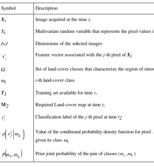
dimensions I×J) acquired in the same geographical area (area of interest) at two different times, t1 and t2, respectively (Table 1 provides a summary of the notations used in the paper). Let _{x be the feature vector associated with the j-th pixel of the ti (i=1,2) image, and} i_j let Ω={ω₁,ω₂,...,ω_C} be the set of C land-cover classes that characterize the geographical area. In developing our approach, we make two important assumptions, which are considered in several approaches to multitemporal classification (Jeon and Landgrebe, 1999; Solberg, 1999). One implies that the land-cover classes present in the area of interest are the same at the two different times (only the spatial distributions of such classes may change over time). The other implies that the two images are acquired in similar periods of the year in order to avoid incoherent responses from the corresponding types of surface covers. In fact, land-cover classes, especially vegetation classes, may present different spectral behaviors depending on the particular season considered.

Let us assume that only the training set T1, corresponding to the first image X1, is available. We aim at classifying the area of interest at the time t2 by exploiting the

information derived from the previous observations X1 and the corresponding training set T1. This process involves the generation of a land-cover map

M

₂

=

{

l

₁2

,l

₂2

,..,l

_I2_×J

}

, where 2

j

l ∈ Ω is the classification label of the j-th pixel at the time t2.

We face this problem by applying the Bayes rule for the minimum error to a “cascade classifier” (Swain, 1978), i.e.

2 j l =ω_m∈ Ω if and only if x , x P max x , x P _m 1_j 2_{j k} 1_j 2_j k         =     ∈ ω ω Ω ω (1)

where Pω_k x1_j,x2_j is the value of the probability that the j-th pixel belongs to class ω_{k at t2,} given the observations x1_j and x2_j. Under the conventional assumption of class-conditional independence (Swain, 1978; Bruzzone et al., 1999), the above decision rule can be rewritten as: 2 j l =ω_m∈ Ω if and only if

(

)

(

)

_               =        

∑

∑

= ∈ = C 1 n k n k 2 j n 1 j C 1 n m n m 2 j n 1 j , P x p x p max , P x p x p k ω ω ω ω ω ω ω ω Ω ω (2)

where pxi_j ω_k is the value of the conditional density function for the pixel i j

x , given the class ω_k∈ Ω , and P

(

ωn,ω_k

)

is the prior joint probability of the pair of classes (ωn,ωk). The

latter term takes into account the temporal correlation between the two images.

On the basis of the previous expression (2), the classification of X2 involves the estimation of the class-conditional densities at time t1, the class-conditional densities at time t2, and the prior joint probability for each possible pair of classes. These estimates cannot be obtained by using classical supervised techniques, as the lack of training data for the second image X2

prevents the conventional application of such techniques. In this context, we adopt a partially unsupervised approach to the estimation of such probabilistic terms. On the one hand, the class-conditional densities at time t1 can be estimated from the available training set T1 by using a supervised approach to density estimation problems (Duda and Hart, 1973). On the other hand, an unsupervised approach based on the EM algorithm (Dempster et al., 1977) is proposed for the estimation of the remaining terms: the class-conditional densities at time t2 and the prior joint probabilities of classes.

3. The proposed partially unsupervised estimation procedure

The proposed estimation procedure is based on the observation that, under the assumption of class-conditional independence over time, the joint density function of images X1 and X2 (i.e., p(X1, X2)) can be described as a mixture density with C×C components (as many components as possible pairs of classes):

(

)

(

)

(

)

∑ ∑

∑ ∑

= = = =         ≅     = C 1 n C 1 m m n m 2 n 1 C 1 n C 1 m m n m n 2 1 2 1 , P X p X p , P , X , X p X , X p ω ω ω ω ω ω ω ω (3)

where X1 and X2 are two multivariate random variables that represent the pixel values (i.e., the feature vector values) in X1 and X2, respectively. In this context, the estimation of the above terms becomes a mixture density estimation problem, which can be solved by applying the EM algorithm (Dempster et al., 1977; Moon, 1996; Shashahani and Landgrebe, 1994; Bruzzone et al., 1999). In particular, we propose an iterative technique based on a specific formulation of the EM algorithm in terms of the prior joint probabilities of classes in the two images considered. This formulation allows one to derive accurate estimates of both the class-conditional densities of classes p

(

X₂ ω_m

)

_{at time t2 and the prior joint probabilities}

(

n, m

)

In order to further explain the presented technique, let us assume that the probability density function of each class can be described by a Gaussian distribution (i.e. by a mean vector µand a covariance matrixΣ ). Under this common assumption (widely adopted for multispectral image classification problems), the estimation of the above-mentioned statistical terms involves the computation of the following vector parameter ϑ (it is worth noting that such an estimation only concerns the X2 image and the prior joint probabilities):

(

) (

)

(

,

) (

,P ,

)

]. P ...., ,... , P , , P , , ,..., , [ C C 1 C C 2 1 1 1 2 C 2 C 2 1 2 1 ω ω ω ω ω ω ω ω Σ µ Σ µ ϑ − = (4)

In this context, it can be proved that the recursive equations to be used in order to estimate the required parameters are (Dempster, 1977):

[ ]

∑ ∑

∑ ∑

× = = × = = +                     = J I 1 j C 1 n 2 j 1 j m n t J I 1 j 2 j C 1 n 2 j 1 j m n t 1 t 2 m x , x , P x x , x , P ω ω ω ω µ ₍₅₎

[ ]

[ ]

∑ ∑

∑ ∑

× = = × = = +             −             = J I 1 j C 1 n 2 j 1 j m n t J I 1 j 2 t 2 m 2 j C 1 n 2 j 1 j m n t 1 t 2 m x , x , P x x , x , P ω ω µ ω ω Σ ₍₆₎

(

)

J

I

x

,

x

,

P

,

P

J I 1 j 2 j 1 j m n t 1 t m n

_×









=

∑

× = +

ω

ω

ω

ω

(7)

where, the superscripts t and t+1 refer to the values of the parameters at the current and next iterations, respectively. Under the adopted assumption of class-conditional independence in the time domain, the term 

     2 j 1 j m n t _{, x ,x}

(

) (

)

(

)

(

) (

)

(

)

∑ ∑

= = =     C 1 n C 1 m m n t m 2 j t n 1 j m n t m 2 j t n 1 j 2 j 1 j m n t , P x p x p , P x p x p x , x , P ω ω ω ω ω ω ω ω ω ω ₍₈₎

It is worth noting that the terms associated with the class-conditional densities pX₁ ω_n at time t1 do not present any superscript, as their values are estimated by using a classical supervised procedure and remain fixed during the estimation process.

It is possible to prove (Dempster, 1977) that, at each iteration, the estimated parameters evolve from their initial values, thus providing an increase in the log-likelihood function

(

₁, ₂ ϑ

)

L X X :

(

)

∑

×

∑ ∑

(

) (

)

(

)

= = =      =I J 1 j C 1 n C 1 m m n m 2 j n 1 j 2 1, log p x px P , L X X ϑ ω ω ω ω ₍₉₎

until a local maximum is reached. The estimates of the parameters obtained at convergence and those achieved by the classical supervised procedure are then substituted into (2) in order to derive the required set of pixel labels M2.

Concerning the initialization of the considered statistical terms, we adopt the following strategies. The initial values of the parameters that characterize the class-conditional densities at time t2 are obtained by exploiting the corresponding values estimated at time t1 by supervised learning, as proposed in (Bruzzone and Fernàndez Prieto, 2001). Concerning the prior joint probabilities, two possible initialization strategies can be followed depending on the prior knowledge available. One can be used in the cases where no prior knowledge exists concerning the possible land-cover transitions that occurred in the area of interest between the two dates considered. In particular, this strategy assigns equal probabilities to each pair of classes. The other strategy can be adopted when the end-user relies on prior information about the temporal evolution of some land-cover classes. Such information can be translated into probabilistic terms by determining if some of the possible land-cover transitions are likely to

have occurred between the two considered dates (e.g., in many cases, urban areas do not change to a forest during short and medium-term time periods; this means that

P(urban,forest)=0). In particular, we can impose explicit constraints on the permitted values

of the prior joint probabilities of classes P

(

ω ,n ωm

)

. Such constraints may be integrated in the

proposed estimation process by fixing the values of the related prior joint probabilities on the basis of the existing knowledge. Then these values remain constant during the iterative estimation process; only the values of the prior joint probabilities for which no information is available are allowed to vary. This results in a more robust and more accurate estimation process.

4. Experimental results and discussion

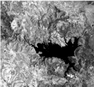
In order to assess the effectiveness of the proposed technique, different experiments were carried out on a data set composed of two multispectral images acquired by the Thematic Mapper (TM) sensor of the Landsat 5 satellite. The selected test site was a section (412×382 pixels) of a scene including Lake Mulargias on the Island of Sardinia, Italy. The two images used in the experiments were acquired in September 1995 (t1) and in July 1996 (t2). Figure 1 shows channels 5 of both images. The available ground truth was used to derive a training set and a test set for each image (see Table 2). In particular, five classes of interest (i.e., pasture, forest, urban area, water body, and vineyard), which characterize the study area over time, were identified. To carry out the experiments, we assumed that only the training set associated with the image acquired in September 1995 was available.

We applied the proposed cascade-classifier approach to the above-described images in order to analyze the July 1996 image by using the estimates of the statistical parameters obtained for the September 1995 image (thanks to the available September 1995 training set), but without using the July 1996 training set. In our experiments, the assumption of normal

distribution was made for the density functions of the classes (this was a reasonable assumption, as we considered TM images).

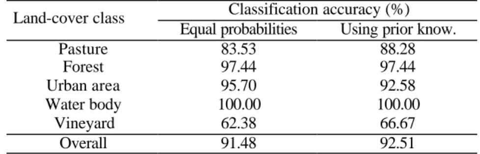
The mean values and the covariance matrices of the Gaussian density functions of the classes at t1 were computed by using the related training set. Concerning the parameters of the density functions of the classes at t2 and the prior joint probabilities of the classes, they were estimated in an unsupervised way by using the proposed formulation of the iterative EM algorithm. In the first experiment, the parameters of the density functions of the classes at t2 were initialized with the values achieved at t1, whereas the values of the prior joint probabilities of the classes were assumed to be the same (no prior information on the land-cover transitions was used in this experiment). The EM algorithm converged in 11 iterations (258 sec on a Sun Workstation Ultra-Sparc 80). At the end of the iterative process, the resulting estimates were used to perform the classification of the July 1996 image. The results obtained are shown in Table 3. As one can see, we obtained a high overall classification accuracy at t2 (i.e., 91.48%), even though the training set was not used. The value of the coefficient of accuracy K (i.e., 0.88) also confirms the effectiveness of the presented technique.

In order to better understand the capabilities of the proposed approach, we carried out a second experiment in which we exploited some a priori information in the initialization of the prior joint probabilities of the classes and, consequently, in the estimation process. In particular, as in the considered region no changes affected the vineyard class between the two dates, we assumed P(vineyard, vineyard)=P(vineyard), whereas all the remaining prior joint probabilities related to the vineyard class were fixed to zero (e.g., P(vineyard,urban)=0,

P(urban,vineyard)=0, etc.). The results obtained by using the above-mentioned prior

information (see Table 3), show a slight increase in the overall classification accuracy (i.e., about 1%) and a sharp increase in the classification accuracy of the vineyard class (i.e., about

4.3%). In addition, the value of the coefficient of accuracy K increased significantly from 0.88 to 0.90. This is also confirmed by a comparison with the accuracies provided by the previous version of the method (Bruzzone and Fernández Prieto, 2001), where no prior knowledge was used. For example, with respect to that method, an increase in the classification accuracy of the vineyard class of about 2.6% was obtained (see (Bruzzone and Fernández Prieto, 2001)).

A further insight into the capabilities of the proposed technique can be derived from Tables 4(a) and 4(b), where the confusion matrices that resulted from the aforementioned experiments are shown. In the matrices, the true land-cover classes (determined according to the ground truth) are given in the rows, and the land-cover classes identified with the proposed technique are given in the columns. Therefore, the values on the diagonals of such matrices represent correctly recognized land-cover classes, while the other values represent errors on the recognition of the classes. As one can see, the use of the prior information about the vineyard class (i.e., P(vineyard, vineyard)=P(vineyard)) in the estimation process resulted in a significant reduction in the omission errors for such a class.

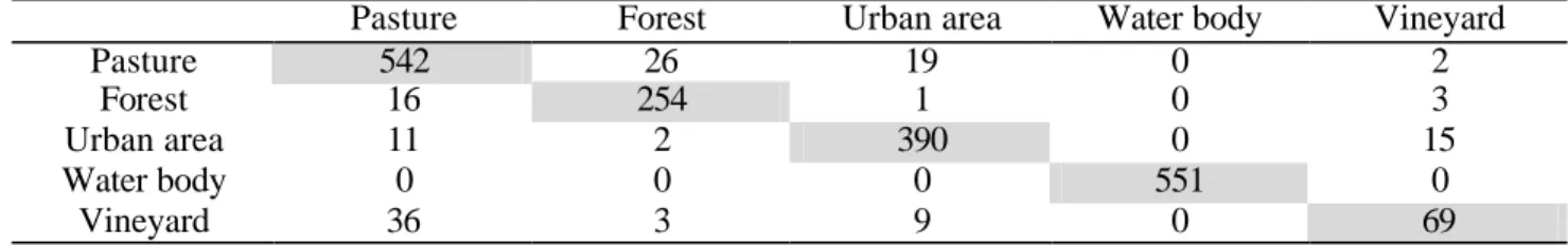
In the third experiment, for the sake of comparison, a supervised ML classifier was trained and subsequently tested on the July 1996 image by the classical approach (i.e., by using a training set for the supervised parameter estimation). The results obtained are presented in Tables 5 and 6, where the classification errors and the confusion matrix are given, respectively. As one can see, the overall classification accuracies achieved by the proposed approach on the July test set (91.48% and 92.51% in Table 3) are very similar to that yielded by the supervised ML classifier (92.66% in Table 5). In greater detail, the accuracies are comparable for all the classes. In addition, the value of the coefficient of accuracy K obtained by the proposed technique when the prior knowledge was used (i.e., 0.90) was equal to the value obtained by the classical supervised approach.

Finally, a further experiment was carried out to assess the accuracies of the initial estimates of the class-conditional densities at time t₂. According to our approach, such estimates were assumed to be equal to the corresponding values obtained for the t₁ image. To this end, a classical ML classifier was trained on the t₁ image (i.e., the September 1995 image). After training, the effectiveness of the classifier was evaluated on the test set of the t₂ image (i.e., the July 1996 image). The classification accuracies obtained (see Table 7) were very low. In particular, the overall classification accuracy for the July test set was equal to 50.43%, which cannot be considered an acceptable result. The meaning of this result is twofold. On the one hand, it highlights the implicit difficulty of the multitemporal data set considered, as the estimates on the September training set proved unsuitable to providing acceptable classification accuracies for the July test set. On the other hand, it confirms the capability of the proposed approach to iteratively improve the accuracies of the estimates of the class-conditional densities at time t₂.

5. Conclusions

In this paper, a partially unsupervised approach to the classification of multitemporal remote-sensing images has been presented. Such an approach allows the classification of a remote-sensing image acquired in a specific geographical area at a given time, in the cases where training data are not available. The classification is performed using the statistical parameters estimated for an image acquired in the same area before the one under analysis.

The proposed method is based on a cascade-classifier approach and on a specific formulation of the EM algorithm. The iterative EM algorithm allows the unsupervised estimation of both the prior joint probabilities of classes and the density functions of classes at time t2 on the basis of the available information: i.e., the known density functions of classes at time t1 (derived from the available training set) and the joint density function p(X1, X2) of

the two images considered. In addition, the proposed technique allows the exploitation of the prior information (if available) about the possible land-cover transitions that occurred in the area of interest between the two considered times; this may increase the robustness of the classification procedure.

It is worth noting that, in some cases, the values of the parameters that characterize the density functions of classes at time t1 may not provide accurate approximations for the same terms at time t2. This may depend on differences in atmospheric and light conditions that alter the spectral signatures of land-cover classes in different images and consequently the distributions of the classes in the feature space. Such differences may lead to the use of initialization values of the parameters of the density functions of classes at t2 significantly different from the true values. Therefore, in these cases, before applying the proposed approach, we recommend performing a simple pre-processing phase aimed at reducing, if possible, the effects of the aforesaid differences. This may provide better starting points for the estimation procedure.

Experiments carried out on a multitemporal data set confirmed the validity of the proposed technique. In particular, they pointed out its capability to accurately estimate the class-conditional densities at time t2 as well as the prior joint probabilities of classes. Consequently, the adopted classifier proved very effective and attained high classification accuracies for the second image, without relying on the corresponding training set.

6. Acknowledgment

7. References

Bruzzone L., Fernàndez Prieto D., and Serpico S. B., “A neural statistical approach to multitemporal and multisource remote-sensing image classification,” IEEE Transactions on Geoscience and

Remote Sensing, vol. 37, no. 3, pp.1350-1359, 1999.

Bruzzone L. and Fernàndez Prieto D., “Unsupervised retraining of a maximum-likelihhod classifier for the analysis of multitemporal remote-sensing images,” IEEE Transactions on Geoscience

and remote Sensing, vol. 39, no. 2, pp. 456-460, 2001.

Dempster A.P., Laird, N.M., and Rubin D.B., “ Maximum likelihood from incomplete data via the EM algorithm,” Journal of Royal Statistic. Soc., vol. 39, no. 1, pp. 1-38, 1977.

Duda R. O. and Hart P. E., Pattern Classification and Scene Analysis. New York: John Wiley & Sons, 1973.

Kalayeh H. M. and Landgrebe D. A., “Utilizing multitemporal data by a stochastic model,” IEEE

Transactions on Geoscience and Remote Sensing, vol. GE-24, no. 5, pp. 792-795, September

1986.

Khazenie N. and Crawford M. M., “Spatial-temporal autocorrelated model for contextual classification,” IEEE Transactions on Geoscience and Remote Sensing, vol. 28, no. 4, pp. 529-539, July 1990.

Jeon B. and Landgrebe D. A., “Classification with spatio-temporal interpixel class dependency contexts,” IEEE Transactions on Geoscience and Remote Sensing, vol. 30, no. 4, pp. 663-672, January 1992.

Jeon B. and Landgrebe D. A., “Data fusion approach to multitemporal classification,” IEEE

Transactions on Geoscience and Remote Sensing, vol. 37, no. 3, pp. 1227-1233, 1999.

Moon T.K., “The Expectation-Maximization algorithm,” Signal Processing Magazine, vol.13, no.6, pp. 47-60, November 1996.

A. H. S. Solberg, “Contextual data fusion applied to forest map revision,” IEEE Transactions on

Geoscience and Remote Sensing, vol. 37, no. 3, pp. 1234-1243, 1999.

Shahshahani B. M. and Langrebe D. A., “The effect of unlabeled samples in reducing the small size problem and mitigating the Hughes phenomenon,” IEEE Transactions on Geoscience and

Remote Sensing, vol. 32, no. 5, pp. 1087-1095, September 1994.

Swain P. H., “Bayesian classification in a time-varying environment,” IEEE Transactions on

(a) (b)

Fig. 1. Bands 5 of the Landsat-5 TM images utilized for the experiments: (a) image acquired in September 1995; (b) image acquired in July 1996.

Table 1. Legend of notations used in this paper

Symbol Description

Xi Image acquired at the time ti

Xi Multivariate random variable that represents the pixel values in Xi

I×J Dimensions of the selected images i

j

x Feature vector associated with the j-th pixel of Xi

Ω Set of land-cover classes that characterize the region of interest

ωi i-th land-cover class

T1 Training set available for time t1

M2 Required Land-cover map at time t2

2

j

l Classification label of the j-th pixel at time t2

    k i j x

p ω Value of the conditional probability density function for pixel xij, given its class ω_k

(

n, k

)

Table 2. Number of patterns in the training and test sets of both the September 1995 and July 1996 images

Number of patterns Land-cover classes

Training set Test set Pasture 554 589 Forest 304 274 Urban area 408 418 Water body 804 551 Vineyard 179 117 Overall 2249 1949

Table 3. Classification accuracies obtained by using the proposed technique with two different initialization strategies for the joint probabilities of classes: a) equal probabilities; b) prior knowledge

of the vineyard class

Classification accuracy (%) Land-cover class

Equal probabilities Using prior know. Pasture 83.53 88.28 Forest 97.44 97.44 Urban area 95.70 92.58 Water body 100.00 100.00 Vineyard 62.38 66.67 Overall 91.48 92.51

Table 4. Confusion matrices that resulted from the classification of the July 1996 test set by using the proposed technique with two different initialization strategies for the joint probabilities of classes: (a)

equal probabilities; (b) prior knowledge of the vineyard class

Pasture Forest Urban area Water body Vineyard Pasture 492 12 85 0 0 Forest 2 267 2 0 3 Urban area 5 5 400 0 8 Water body 0 0 0 551 0 Vineyard 23 11 10 0 73 (a)

Pasture Forest Urban area Water body Vineyard Pasture 520 13 56 0 0 Forest 2 267 2 0 3 Urban area 7 7 387 0 17 Water body 0 0 0 551 0 Vineyard 22 9 8 0 78 (b)

Table 5. Classification accuracies obtained on the July 1996 test set by using a classical supervised ML classifier trained for the July 1996 training set

Land-cover class Classification accuracy (%) Pasture 92.02 Forest 92.70 Urban area 93.30 Water body 100.00 Vineyard 58.97 Overall 92.66

Table 6. Confusion matrix that resulted from the classification of the July 1996 test set by using a classical supervised ML classifier trained on the July 1996 training set

.

Pasture Forest Urban area Water body Vineyard Pasture 542 26 19 0 2

Forest 16 254 1 0 3 Urban area 11 2 390 0 15 Water body 0 0 0 551 0

Vineyard 36 3 9 0 69

Table 7. Classification accuracies obtained for the July 1996 test set by using a classical supervised ML classifier trained on the September 1995 training set

Land-cover class Classification accuracy (%) Pasture 19.52 Forest 95.62 Urban area 90.43 Water body 36.11 Vineyard 24.78 Overall 50.43