Encoding the satisfiability of modal and description logics into SAT: the case study of K(m)/ALC

(1)

UNIVERSITY

OF TRENTO

DEPARTMENT OF INFORMATION AND COMMUNICATION TECHNOLOGY

38050 Povo – Trento (Italy), Via Sommarive 14

http://www.dit.unitn.it

ENCODING THE SATISFIABILITY OF MODAL AND

DESCRIPTION LOGICS INTO SAT: THE CASE STUDY OF

K(M)/ALC

Roberto Sebastiani and Michele Vescovi

May 2006

(2)

(3)

Encoding the satisfiability of modal and description

logics into SAT: the case study of K(m)/

ALC

Roberto Sebastiani and Michele Vescovi

DIT, Universit`a di Trento, Via Sommarive 14, I-38050, Povo, Trento, Italy.

roberto.sebastiani@dit.unitn.it, michele.vescovi@studenti.unitn.it

Abstract. In the last two decades, modal and description logics have been

ap-plied to numerous areas of computer science, including artificial intelligence, formal verification, database theory, and distributed computing. For this reason, the problem of automated reasoning in modal and description logics has been throughly investigated.

In particular, many approaches have been proposed for efficiently handling the satisfiability of the core normal modal logic Km, and of its notational variant, the description logicALC. Although simple in structure, Km/ALC is computation-ally very hard to reason on, its satisfiability being PSPACE-complete.

In this paper we explore the idea of encoding Km/ALC-satisfiability into SAT, so that to be handled by state-of-the-art SAT tools. We propose an efficient encoding, and we test it on an extensive set of benchmarks, comparing the approach with the main state-of-the-art tools available.

Although the encoding is necessarily worst-case exponential, from our experi-ments we notice that, in practice, this approach can handle most or all the prob-lems which are at the reach of the other approaches, with performances which are comparable with, or even better than, those of the current state-of-the-art tools.

1 Introduction

In the last two decades, modal and description logics have been applied to numerous areas of computer science, including artificial intelligence, formal verification, database theory, and distributed computing. For this reason, the problem of automated reasoning in modal and description logics has been throughly investigated (see, e.g., [5, 17, 10, 18]). Many approaches have been proposed for efficiently handling the satisfiability of modal and description logics, in particular of the core normal modal logic Kmand of its notational variant, the description logic

ALC

(see, e.g., [5, 18, 7, 8, 12, 15, 14, 3, 19, 20]). Notice that, although simple in structure, Km/

ALC

is computationally very hard to reason on, as its satisfiability is PSPACE-complete [17, 10].

In this paper we explore the idea of encoding Km/

ALC

-satisfiability into SAT, so that to be handled by state-of-the-art SAT tools. We propose an efficient encoding, with four simple variations. We test (the four variations of) it on an extensive set of benchmarks, comparing the results with those of the main state-of-the-art tools for Km -satisfiability available.

Although the encoding is necessarily worst-case exponential (unless PSPACE=NP), from our experiments we notice that, in practice, this approach can handle most or all

(4)

the problems which are at the reach of the other approaches, with performances which are comparable with, or even better than, those of the current state-of-the-art tools.

Related work. First, we briefly overview the most successful approaches for the satisfiability of modal logics, and of Kmin particular. The “classic” tableau-based ap-proach [5, 17, 10, 18] is based on the construction of propositional tableau branches, which are recursively expanded on demand by generating successor nodes in a candi-date Kripke model. (Tools based on this approach are no more state-of-the-art.) In the

SAT-based approach [7, 8] a DPLL procedure, which treats the modal subformulas as

propositions, is used as boolean engine at each nesting level of the modal operators: when a satisfying assignment is found, the corresponding set of modal subformulas is recursively checked for modal consistency. Among the tools employing (and extending) this approach, we recall KSAT [7, 6], *SAT [25], FACT and DLP [12], and RACER [26].1 _{In the translational approach [15, 1] the modal formula is encoded into} first-order logic (FOL), and the encoded formula can be decided efficiently by a FOL the-orem prover [1]. MSPASS[14] is the most representative tool of this approach. In the

Automata-theoretic approach, (a BDD-based symbolic representation of) a tree

automa-ton accepting all the tree models of the input formula is implicitly built and checked for emptiness [19, 20]. KBDD [20] is the representative tool of this approach. [20] presents also an encoding of K-satisfiability into QBF-satisfiability (that is a PSPACE-complete problem too), combined with the use of a state-of-the-art QBF solver.

Moreover, we briefly recall some approaches based on SAT encoding which have been successful in other domains: planning has been fruitfully encoded into SAT [16], and a similar encoding has been proposed for the problem of (bounded) LTL model checking [2]; in both cases, these approaches are currently state-of-the-art in the re-spective communities. Effective encodings into SAT have been proposed also for the satisfiability problems in some quantifier-free FOL theories which are of interest for formal verification, including these of separation logic (SL) [24], of SL with equality

and uninterpreted functions [22], and of linear arithmetic [23].

Structure of the paper. In §2 we provide the necessary background notions. In §3 we describe the encoding, and provide some examples. In §4 we present an exten-sive empirical evaluation, and discuss the results. In §5 we conclude, an describe some possible future evolutions.

2 Background

We recall some basic definitions and properties of Km. Given a non-empty set of prim-itive propositions

A

= {A1, A2, . . .} and a set of m modal operators

B

= {21, . . . , 2m}, the language of Km is the least set of formulas containing

A

, closed under the set of propositional connectives {¬, ∧} and the set of modal operators in

B

. Notation-ally, we use the Greek letters α, β, ϕ, ψ, ν, π to denote formulas in the language of

Km (Km-formulas hereafter). We use the standard abbreviations, that is: “3rϕ” for “¬2r¬ϕ”, “ϕ1∨ϕ2” for “¬(¬ϕ1∧¬ϕ2)”, “ϕ1→ ϕ2” for “¬(ϕ1∧¬ϕ2)”, “ϕ1↔ ϕ2” for

1_{Notice that, for historical reasons, tools like F}_A_{CT, DLP, and R}_ACER_{are called “tableau”,}

(5)

“¬(ϕ1∧ ¬ϕ2) ∧ ¬(ϕ2∧ ¬ϕ1)”, “>” and “⊥” for the constants “true” and “false”. (Here-after formulas like ¬¬ψ are implicitly assumed to be simplified into ψ, so that, if ψ is

¬φ, then by “¬ψ” we mean “φ”.) We call depth of ϕ, written depth(ϕ), the maximum

number of nested modal operators in ϕ. We call a propositional atom every primitive proposition in

A

, and a propositional literal every propositional atom (positive literal) or its negation (negative literal).

In order to make our presentation more uniform, we adopt from [5, 18] the repre-sentation of Km-formulas from the following table:

α α1 α2 β β1 β2 πr πr0 νr νr0

(ϕ1∧ ϕ2) ϕ1 ϕ2 (ϕ1∨ ϕ2) ϕ1 ϕ2 3rϕ1 ϕ1 2rϕ1 ϕ1

¬(ϕ1∨ ϕ2) ¬ϕ1 ¬ϕ2 ¬(ϕ1∧ ϕ2) ¬ϕ1¬ϕ2 ¬2rϕ1¬ϕ1 ¬3rϕ1¬ϕ1

, u |= β1or

M

, u |= β2;

M

, u |= πr _⇐⇒

_M

_{, w |= π}r

0for some w ∈

U

s.t.

R

r(u, w) holds in

M

;

M

, u |= νr _⇐⇒

_M

_{, w |= ν}r

0for every w ∈

we sometimes drop the prefix “Km-”.) We say that w is a successor of u through

R

riff

R

r(u, w) holds in

M

.

The problem of determining the Km-satisfiability of a Km-formula ϕ is decidable and PSPACE-complete [17, 10], even restricting the language to a single boolean atom (i.e.,

A

= {A1}) [9]; if we impose a bound on the modal depth of the Km-formulas, the prob-lem reduces to NP-complete [9]. For a more detailed description on Km— including, e.g., axiomatic characterization, decidability and complexity results — see [10, 9].

A Km-formula is said to be in Negative Normal Form (NNF) if it is written in terms of the symbols 2r, 3r, ∧, ∨ and propositional literals Ai, ¬Ai(i.e., if all negations occur only before propositional atoms in

A

). Every Km-formula ϕ can be converted into an equivalent one NNF(ϕ) by recursively applying the rewriting rules: ¬2rϕ=⇒3r¬ϕ,

¬3rϕ=⇒2r¬ϕ, ¬(ϕ1∧ ϕ2)=⇒(¬ϕ1∨ ¬ϕ2), ¬(ϕ1∨ ϕ2)=⇒(¬ϕ1∧ ¬ϕ2), ¬¬ϕ=⇒ϕ. A Km-formula is said to be in Box Normal Form (BNF) [19, 20] if it is written in terms of the symbols 2r, ¬2r, ∧, ∨, and propositional literals Ai, ¬Ai (i.e., if no diamonds are there, and all negations occurs only before boxes or before propositional atoms in

A

). Every Km-formula ϕ can be converted into an equivalent one BNF(ϕ) by

(6)

recursively applying the rewriting rules: 3rϕ=⇒¬2r¬ϕ, ¬(ϕ1∧ ϕ2)=⇒(¬ϕ1∨ ¬ϕ2),

¬(ϕ1∨ ϕ2)=⇒(¬ϕ1∧ ¬ϕ2), ¬¬ϕ=⇒ϕ.

3 The Encoding

We borrow some notation from the Single Step Tableau (SST) framework [18, 4]. We represent univocally states in

M

as labels σ, represented as non empty sequences of integers 1.nr1

1.nr22. ... .nrkk, s.t. the label 1 represents the root state, and σ.nr represents the n-th successor of σ through the relation

R

r. With a little abuse of notation, hereafter we may say “a state σ” meaning “a state labeled by σ”.

Notationally, we often write “(V_ili) → W

jlj” for the clause “ W j¬li∨ W jlj”, and “(V_ili) → ( V

jlj)” for the conjunction of clauses “ V

j( W

i¬li∨ lj)”.

3.1 The Basic Encoding

Let A_{[, ]}be an injective function which maps a pair hσ, ψi, s.t. σ is a state label and ψ is a Km-formula which is not in the form ¬φ, into a boolean variable A[σ, ψ]. Let L[σ, ψ] denote ¬A[σ, φ] if ψ is in the form ¬φ, A[σ, ψ] otherwise. Given a Km-formula ϕ, the encoder Km2SAT builds a boolean CNF formula as follows:

Km2SAT (ϕ) := A[1, ϕ]∧ De f (1, ϕ), (1) De f (σ, Ai), := > (2) De f (σ, ¬Ai) := > (3) De f (σ, α) := (L_{[σ, α]}→ (L_{[σ, α}₁_]∧ L_{[σ, α}₂_])) ∧ De f (σ, α1) ∧ De f (σ, α2) (4) De f (σ, β) := (L[σ, β]→ (L[σ, β1]∨ L[σ, β2])) ∧ De f (σ, β1) ∧ De f (σ, β2) (5) De f (σ, πr, j) := (L_{[σ, π}r, j_]→ L [σ. j, πr, j0 ]) ∧ De f (σ. j, π r, j 0 ) (6) De f (σ, νr) := ^ hσ:πr,i_i ((L[σ, νr_]∧ L_{[σ, π}r,i_]) → L_{[σ.i, ν}r 0]) ∧ ^ hσ:πr,i_i De f (σ.i, νr₀). (7)

We assume that the Km-formulas are represented as DAGs, so that to avoid the expan-sion of the same De f (σ, ψ) more than once. Moreover, following [18], we assume that, for each σ, the De f (σ, ψ)’s are expanded in the order: α, β, π, ν. Thus, each De f (σ, νr₎ is expanded after the expansion of all De f (σ, πr,i_{)’s, so that De f (σ, ν}r_{) will generate} one clause ((L_{[σ, π}r,i_]∧ L_[σ,₂_r_νr

0]) → L[σ.i, νr0]) and one novel definition De f (σ.i, ν

r 0) for each De f (σ, πr,i_{) expanded.}

Intuitively, it is easy to see that Km2SAT (ϕ) mimics the construction of an SST tableau expansion [18, 4]. We have the following fact.

Theorem 1. A Km-formula ϕ is Km-satisfiable if and only if the corresponding boolean

formula Km2SAT (ϕ) is satisfiable.

The complete proof of Theorem 1 can be found in the Appendix.

Notice that, due to (7), the number of variables and clauses in Km2SAT (ϕ) may grow exponentially with depth(ϕ). This is in accordance to what stated in [9].

(7)

3.2 Variants

Before the encoding, some potentially useful preprocessing can be performed.

First, the input Km-formulas can be converted into NNF (like, e.g., in [18, 4]) or into BNF (like, e.g., in [7, 19]). One potential advantage of the latter is that, when one

2rψ occurs both positively and negatively (like, e.g., in (2rψ ∨ ...) ∧ (¬2rψ ∨ ...) ∧ ...), then both occurrences of 2rψ are labeled by the same boolean atom A[σ,2rψ], and hence

they are always assigned the same truth value by DPLL; with NNF, instead, the negative occurrence ¬2rψ is rewritten into 3r¬ψ, so that two distinct boolean atoms A[σ,2rψ]

and A[σ,3r¬ψ]are generated; DPLL can assign them the same truth value, creating a

hidden conflict which may require some extra boolean search to reveal.

Example 1 (NNF). Let ϕnn f be (3A1∨ 3(A2∨ A3)) ∧ 2¬A1 ∧ 2¬A2 ∧ 2¬A3.2It is easy to see that ϕnn f is K1-unsatisfiable. Km2SAT (ϕnn f) is:

1. A[1, ϕnn f]

2. ∧ ( A_{[1, ϕ}_{nn f}_]→ (A_[1,3A1∨3(A2∨A3)]∧ A[1,2¬A1]∧ A[1,2¬A2]∧ A[1,2¬A3]) ) 3. ∧ ( A[1,3A1∨3(A2∨A3)]→ (A[1,3A1]∨ A[1,3(A2∨A3)]) ) 4. ∧ ( A_[1,3A1]→ A[1.1, A1]) 5. ∧ ( A[1,3(A2∨A3)]→ A[1.2, A2∨A3]) 6. ∧ ( (A[1,2¬A1]∧ A[1,3A1]) → ¬A[1.1, A1]) 7. ∧ ( (A_[1,2¬A2]∧ A[1,3A1]) → ¬A[1.1, A2]) 8. ∧ ( (A[1,2¬A3]∧ A[1,3A1]) → ¬A[1.1, A3]) 9. ∧ ( (A[1,2¬A1]∧ A[1,3(A2∨A3)]) → ¬A[1.2, A1]) 10. ∧ ( (A_[1,2¬A2]∧ A[1,3(A2∨A3)]) → ¬A[1.2, A2]) 11. ∧ ( (A[1,2¬A3]∧ A[1,3(A2∨A3)]) → ¬A[1.2, A3]) 12. ∧ ( A_{[1.2, A}₂_∨A₃_]→ (A_{[1.2, A}₂_]∨ A_{[1.2, A}₃_]) )

After a run of BCP, 3. reduces to a disjunction. If the first element A[1,3A1]is assigned, then by BCP we have a conflict on 4.,6. If the second element A[1,3(A2∨A3)]is assigned, then by BCP we have a conflict on 12. Thus Km2SAT (ϕnn f) is unsatisfiable. ¦

Example 2 (BNF). Let ϕbn f = (¬2¬A1∨ ¬2(¬A2∧ ¬A3)) ∧ 2¬A1 ∧ 2¬A2 ∧ 2¬A3. It is easy to see that ϕbn f is K1-unsatisfiable. Km2SAT (ϕbn f) is: 3

2_{For K}

1formulas, we omit the box and diamond indexes.

(8)

1. A[1, ϕbn f]

2. ∧ ( A[1, ϕbn f]→ (A[1, (¬2¬A1∨¬2(¬A2∧¬A3))]∧ A[1,2¬A1]∧ A[1,2¬A2]∧ A[1,2¬A3]) ) 3. ∧ ( A_{[1, (¬}2¬A1∨¬2(¬A2∧¬A3))]→ (¬A[1,2¬A1]∨ ¬A[1,2(¬A2∧¬A3)]) )

4. ∧ ( ¬A[1,2¬A1]→ A[1.1, A1])

5. ∧ ( ¬A_[1,2(¬A2∧¬A3)]→ ¬A[1.2, (¬A2∧¬A3)]) 6. ∧ ( (A[1,2¬A1]∧ ¬A[1,2¬A1]) → ¬A[1.1, A1]) 7. ∧ ( (A[1,2¬A2]∧ ¬A[1,2¬A1]) → ¬A[1.1, A2]) 8. ∧ ( (A_[1,2¬A3]∧ ¬A[1,2¬A1]) → ¬A[1.1, A3]) 9. ∧ ( (A[1,2¬A1]∧ ¬A[1,2(¬A2∧¬A3)]) → ¬A[1.2, A1]) 10. ∧ ( (A[1,2¬A2]∧ ¬A[1,2(¬A2∧¬A3)]) → ¬A[1.2, A2]) 11. ∧ ( (A_[1,2¬A3]∧ ¬A[1,2(¬A2∧¬A3)]) → ¬A[1.2, A3]) 12. ∧ ( ¬A[1.2, (¬A2∧¬A3)]→ (A[1.2, A2]∨ A[1.2, A3]) )

Unlike with NNF, Km2SAT (ϕbn f) is found unsatisfiable directly by BCP. Notice that the unit-propagation of A_[1,2¬A1]from 2. causes ¬A[1,2¬A1]in 3. to be false, so that one of the two (unsatisfiable) branches induced by the disjunction is cut a priori. With NNF, the corresponding atoms A_[1,2¬A1]and A[1,3A1]are not recognized to be one the nega-tion of the other, s.t. DPLL may need exploring one boolean branch more. ¦

Second, the (NNF or BNF) Km-formula can also be rewritten by recursively apply-ing the validity-preservapply-ing “box/diamond liftapply-ing rules”:

(2rϕ1∧ 2rϕ2) =⇒ 2r(ϕ1∧ ϕ2), (3rϕ1∨ 3rϕ2) =⇒ 3r(ϕ1∨ ϕ2). (8) This has the potential benefit of reducing the number of πr,i formulas, and hence the number of labels σ.i to take into account in the expansion of the De f (σ, νr_{)’s (7).}

Example 3 (NNF with LIFT). Let ϕnn f li f t = 3(A1∨ A2∨ A3) ∧ 2(¬A1∧ ¬A2∧ ¬A3). It is easy to see that ϕbn f li f t is K1-unsatisfiable. Km2SAT (ϕbn f li f t) is:

A_{[1, ϕ}_{nn f li f t}_]

∧ ( A[1, ϕnn f li f t]→ (A[1,3(A1∨A2∨A3)]∧ A[1,2(¬A1∧¬A2∧¬A3)]) )

∧ ( A[1,3(A1∨A2∨A3)]→ A[1.1, A1∨A2∨A3])

∧ ( (A_[1,2(¬A1∧¬A2∧¬A3)]∧ A[1,3(A1∨A2∨A3)]) → A[1.1, (¬A1∧¬A2∧¬A3)])

∧ ( A[1.1, A1∨A2∨A3]→ (A[1.1, A1]∨ A[1.1, A2]∨ A[1.1, A3]) )

∧ ( A[1.1, (¬A1∧¬A2∧¬A3)]→ (¬A[1.1, A1]∧ ¬A[1.1, A2]∧ ¬A[1.1, A3]) )

Km2SAT (ϕnn f li f t) is found unsatisfiable by BCP. ¦

Example 4 (BNF with LIFT). Let ϕbn f li f t = ¬2(¬A1∧ ¬A2∧ ¬A3) ∧ 2(¬A1∧ ¬A2∧ ¬A3). It is easy to see that ϕbn f li f t is K1-unsatisfiable. Km2SAT (ϕbn f li f t) is:

1. A_{[1, ϕ}_{bn f li f t}_]

2. ∧ ( A_{[1, ϕ}_{bn f li f t}_]→ (¬A_[1,2(¬A1∧¬A2∧¬A3)]∧ A[1,2(¬A1∧¬A2∧¬A3)]) ) 3. ∧ ( ¬A[1,2(¬A1∧¬A2∧¬A3)]→ ¬A[1.1, (¬A1∧¬A2∧¬A3)])

4. ∧ ( ¬A_{[1.1, (¬A}₁_∧¬A₂_∧¬A₃_)]→ (A_{[1.1, A}₁_]∨ A_{[1.1, A}₂_]∨ A_{[1.1, A}₃_]) )

Km2SAT (ϕbn f li f t) is found unsatisfiable by BCP. ¦ One potential drawback of applying the lifting rules is that, by collapsing (2rϕ1∧

2rϕ2) into 2r(ϕ1∧ ϕ2) and (3rϕ1∨ 3rϕ2) into 3r(ϕ1∨ ϕ2), the possibility of sharing box/diamond subformulas in the DAG representation of ϕ is reduced.

(9)

4 Empirical Evaluation

In order to verify empirically the effectiveness of this approach, we have performed an extensive empirical test session. We have implemented the encoder Km2SAT in C++, with two flags: NNF/BNF, performing a pre-conversion into NNF/BNF before the en-coding, and lift/nolift, performing box lifting before the encoding. We have tried many SAT solvers on our encoded formulas (including ZCHAFF2004.11.15, SIEGE v4, BERKMIN5.6.1, MINISATv1.13, SAT-ELITEv1.0 and SAT-ELITEGTI 2005 submission). ). After a preliminary evaluation, we have selected ZCHAFFand SAT-ELITEGTI (hereafter SAT-ELITE).

Among the state-of-the-art tools for Km-satisfiability, we have selected RACER[26] and *SAT [25] as the best representers of the tableaux/DPLL-based tools, MSPASS [15, 14] as the best representer of the FOL-encoding approach, 4 _{KBDD [19, 20]} 5 as the representer of the automata-theoretic approach, and the K-QBF translator [20] combined with the SEMPROPQBF solver (which seems to be the best QBF solver for these kinds of problems 6_{) as representant of the QBF-encoding approach.} 7

All tests presented in this section have been performed on a two-processor Intel Xeon 3.0GHz computer, with 1 MByte Cache each processor, 4 GByte RAM, with Red Hat Linux 3.0 Enterprise Server, where four processes can run in parallel. When reporting the results for one Km2SAT +DPLL version, the CPU times reported are the sums of both the encoding and DPLL solving times.

In order to make the results reproducible, the encoder, the benchmarks and the files with all the plots are available.8

4.1 Test description

As a first group of benchmark formulas we used the LWB benchmark suite used in a comparison at Tableaux’98 [11]. It consists on 9 classes of parameterized formulas (each in two versions, valid “ p” or invalid “ n”), for a total amount of 378 formulas. The parameter allows for creating formulas of increasing size and difficulty.

The benchmark methodology is to test formulas from each class, in increasing dif-ficulty, until one formula cannot be solved within a given timeout (1000 seconds in our tests)9_{. The result from this class is the parameter’s value of the largest (and hardest)} formula that can be solved within the time limit. (The parameter ranges only from 1 to

4_{We have run} _M_SPASS _{with the options -EMLTranslation=2 -EMLFuncNary=1}

-Sorts=0 -CNFOptSkolem=0 -CNFStrSkolem=0 -Select=2 -Split=-1 -DocProof=0

-PProblem=0 -PKept=0 -PGiven=0, which are suggested for Km-formulas in the MSPASS

README file.

5_{KBDD has been run with the default internal memory bound of 384MB.}

6_{In results we report only S}_EMPROP_{times, since the time spent by K-QBF is almost}

negli-giable.

7_{Other tools like}_LEAN_{K, 2KE, LWB, K}_RIS_{are not competitive with the ones listed above}

[13]. Tools like DLP and FACT are similar in spirit and performances to RACERand *SAT.

KSAT [7, 8, 6] has been reimplemented into *SAT.

8_{Available at http://www.dit.unitn.it/˜rseba/sat06/allmaterial.tar.gz.}

9_{We also set a 1GB file-size limit for the encoding produced by K}

(10)

21 so that, if a system can solve all 21 instances of a class, the result is given as 21.) For a discussion on this benchmark suite, we refer the reader to [11, 13].

As a second group of benchmark formulas, we have selected the random 2m-CNF testbed described in [13, 21]. This is a generalization of the well-known random k-SAT test methods, and is the final result on a long discussion in the communities of modal and description logics on how to to obtain significant and flawless random benchmarks for modal/description logics (see [7, 15, 6, 13, 21]).

In the 2m-CNF test methodology, a 2m-CNF formula is randomly generated ac-cording to the following parameters:

– the (maximum) modal depth d;

– the number of top-level clauses L;

– the number of literal per clause clauses k;

– the number of distinct propositional variables N;

– the number of distinct box symbols m;

– the percentage p of purely propositional literals in clauses occurring at depth < d.10 (We refer the reader to [13, 21] for a more detailed description.)

A typical problem set is characterized by fixed values of d, k, N, m, and p: L is varied in such a way as to empirically cover the “100% satisfiable—100% unsatisfiable” transition. Then, for each tuple of the five values in a problem set, a certain number of

2m-CNF formulas are randomly generated, and the resulting formulas are given in input to the procedure under test, with a maximum time bound. The fraction of formulas which were solved within a given timeout, and the median/percentile values of CPU times are plotted against the ratio L/N. Also, the fraction of satisfiable/unsatisfiable formulas is plotted for a better understanding.

Following [13, 21], we have fixed m = 1, k = 3 and 100 samples/point in all our tests, and we have selected two groups: d = 1, p = 0.5, and N = 6, 7, 8, 9, L/N = 10..60, and

d = 2, p = 0.5, 0.6, N = 3, 4, L/N = 30..150, for a total amount of 12,000 formulas. In

each test, we imposed a timeout of 500 seconds per sample11_{and we plot the number} of samples which were solved within the timeout, and the 50%th and 90%th percentiles of CPU time. In order to correlate the performances with the (un)satisfiability of the sample formulas, in the background of each plot we plot the satisfiable/unsatisfiable ratio.

For both benchmark suites, for all formulas, all tools under test —both all the vari-ants of Km2SAT +DPLL and all the state-of-the-art Km-satisfiability solvers— agreed on the satisfiability/unsatisfiability result when terminating within the timeout. 4.2 An empirical comparison of the different variants of Km2SAT

We have evaluated the four variants of the encoding, with both ZCHAFF and SAT-ELITE.

10_{Each modal clause of length k contains on average p · k randomly-picked boolean literals and}

k − p·k randomly-generated modal literals 2rψ, ¬2rψ. More precisely, the number of boolean

literals in a clause is bp·kc (resp. dp·ke) with probability dp·ke− p·k (resp. 1−(dp·ke− p·k)). Notice that typically the smaller is p, the harder is the problem [13, 21].

11_{With also a 512MB file-size limit for the encoding produced by K}

(11)

number of variables (·103) number of clauses (·103) ZCHAFF SAT-ELITE

Encoding NNF BNF NNF BNF NNF BNF NNF BNF

Lifting yes no yes no yes no yes no yes no yes no yes no yes no

k branch n 1000 1000 1000 1000 1000 1000 1000 1000 4 4 4 4 4 4 4 4 k branch p 1000 1000 1000 1000 1000 1000 1000 1000 4 4 4 4 4 4 4 4 k d4 n 500 2000 2000 1000 600 2000 3000 2000 4 4 6 6 5 6 5 5 k d4 p 5000 5000 9000 9000 6000 6000 11000 11000 9 9 9 9 9 9 10 10 k dum n 5000 5000 5000 5000 6000 6000 6000 6000 18 18 18 18 18 18 18 17 k dum p 7000 7000 5000 6000 8000 9000 7000 7000 17 17 17 17 16 16 16 15 k grz n 10 10 10 10 10 10 10 10 21 21 21 21 21 21 21 21 k grz p 10 10 9 8 10 10 9 8 21 21 21 21 21 21 21 21 k lin n 30 30 30 30 50 50 500 50 21 21 21 21 21 21 21 21 k lin p 4 10 4 10 5 10 5 10 21 21 21 21 21 21 21 21 k path n 2000 2000 2000 2000 2000 2000 2000 2000 5 5 5 6 6 6 6 6 k path p 2000 12000 2000 11000 2000 14000 2000 13000 7 7 7 7 7 8 7 8 k ph n 300 50 300 50 300 50 300 50 21 21 21 21 21 21 21 21 k ph p 10 4 10 5 10 5 10 6 11 11 11 12 11 11 10 11 k poly n 20 200 20 200 20 200 20 200 21 21 21 21 21 21 21 21 k poly p 20 200 20 200 20 200 20 200 21 21 21 21 21 21 21 21 k t4p n 800 1000 3000 4000 900 1000 3000 4000 4 4 5 5 4 4 5 4 k t4p p 3000 3000 4000 4000 3000 4000 4000 5000 8 8 9 9 8 8 9 9

Table 1. Comparison of the variants of Km2SAT +ZCHAFF/SAT-ELITEon the LWB benchmarks.

The results on the LWB benchmark are summarized in Table 1. The first block reports the number of variables and clauses of Km2SAT (ϕ) (referring to the highest case solved). The second block reports the maximum parameter’s value of the hardest formula solved within the timeout. (E.g., the BNF-nolifting encoding of k d4 p(10) contains 9 · 106_{variables and 11 · 10}6_{clauses, it is the hardest k d4 p problem solved} by SAT-ELITE, and it is the first which is not solved by ZCHAFF.)

Looking at the number of clauses and variables, we notice a few facts: first, lifting in many cases reduces the size of the encoded formula (e.g., in k path p), with a few exceptions (e.g., in k grz p); second, BNF in many cases produces smaller formulas than NNF (e.g., in k dum p), with a few exceptions (e.g., in k ph p).

Looking at the CPU times, we notice that the performance gaps are rather small, and there is no absolute winner neither between the SAT solvers nor among the en-codings, although the BNF-nolifting version with ZCHAFFseems to behave slightly better than the others on the whole. We also notice that there seems not to be an absolute correlation between a reduction in size of the encoded formula and an improvement of performances. (E.g., with k path p and BNF, lifting reduces significantly the size of the formula, but it causes a worse performance of SAT-ELITE.)

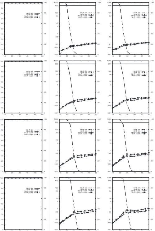
In the random 2m-CNF benchmarks the gaps are more relevant. (For better read-ability, we report only the results for ZCHAFFbecause it turned out to be significantly better then SAT-ELITE on these formula, with a noteworthy exception of the second row in Figure 4, where we reported also the values for SAT-ELITE.)

(12)

For lack of space, we do not present the plots of the number of variables and clauses of the encoded formulas. Anyway, we report a few facts: first, in all the tests, these values grow linearly (or slightly sub-linearly12_{) with the number of clauses L of the K}

m -formula; second, the values are very regular: the gaps between 50% and 90% percentiles are negligible; third, BNF produces slightly smaller formulas than NNF in most cases, but the gaps are small; fourth, lifting increases significantly the number of variables and clauses generated. 13 _{To give a coarse idea of the values, with the hardest problems} (d = 2, p = 0.5, N = 4, L/N = 150) and the worst encoder (lift, NNF), we have about 2.5 · 106_{clauses and 1.5 · 10}6_{variables, whilst with the best encoder (nolift, BNF) we} have about 1.2 · 106_{clauses and 0.7 · 10}6_variables.

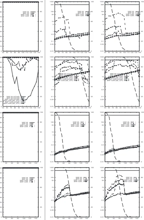
The CPU times are reported in Figures 1 and 2. The tests of Figure 1 are simply too easy for Km2SAT +ZCHAFF (but not for its competitors, see later) which solved every sample formula in less than 1 second. The tests of Figure 2 are more challenging. In general, it seems that in the majority of cases nolifting beats lifting and BNF beats NNF, although this seems not to be a general rule. In the hardest benchmark with

p = 0.5 and N = 4 (2nd row), we also reported the SAT-ELITEplots, because it beats significantly ZCHAFF.

Finally, we notice that for Km2SAT +ZCHAFFthe problems tend to be harder within the satisfiability/unsatisfiability transition area. This fact holds also for RACER and *SAT, see figures 1 and 2. This seems to confirm the fact that the easy-hard-easy pattern of random k-SAT extends also to 2m-CNF, as already observed in [7, 8, 6, 13, 21]. 4.3 An empirical comparison wrt. other approaches

We have evaluated the Km2SAT +DPLL approach against the other Km-satisfiability solvers listed above.

The results on the LWB benchmark are summarized in Table 2. We notice a few facts: first, RACERand *SAT are the best scorers (confirming the analysis in [13]); sec-ond, there is no definite winner between KBDD and MSPASS; third, K-QBF +SEMPROP is the worst performer among the state-of-the-art tools, way below the performances of RACERand *SAT; fourth, Km2SAT +DPLL is the worst performer on k branch, k d4, k dum the second worst performer on k path, k t4p, it equals the competitors on k grz and k lin, and it is (one of) the best performer(s) on k ph and k Pol.

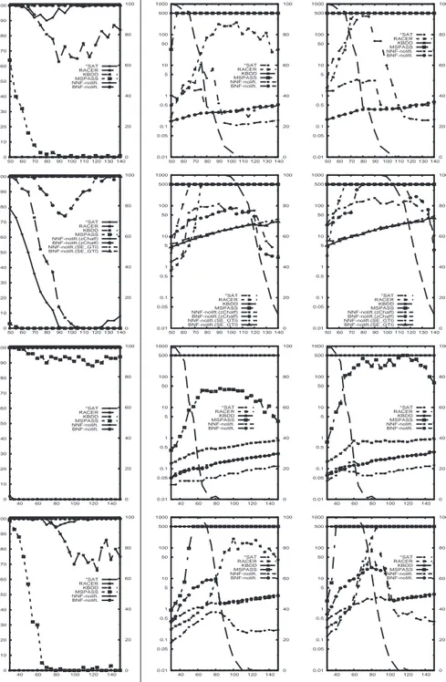
In the random 2m-CNF benchmarks the results are much better for Km2SAT . In Fig-ure 3 (center and right) Km2SAT +ZCHAFFis nearly always the best scorer, followed by *SAT and RACER. From Figure 3 (left) notice that K-QBF +SEMPROP, MSPASS, and KBDD do not terminate within the timeout for most values, whilst Km2SAT +ZCHAFF always terminates (below 1 second). In Figure 4 (center and right) we notice that, for

p = 0.5 (1st and 2nd row) Km2SAT +ZCHAFFis nearly always the best scorer (notice that with N = 4 SAT-ELITEbeats ZCHAFF); for p = 0.6 (3rd and 4th row) Km2SAT +ZCHAFFis beaten only by *SAT. In all these tests, K-QBF +SEMPROP, MSPASSand KBDD are not competitive.

12_{The more clauses are a in 2}

m-CNF formula, the higher are the chances of sharing

sub-formulas.

13_{We believe that this may be due to the fact that random 2}

m-CNF formulas may contain lots of

(13)

state-of-the-art tools Km2SAT best

K-QBF (BNF-nolift + ZCHAFF)

test + SEMPROPKBDD MSPASSRACER*SAT solved encoded

k branch n 10 8 10 15 14 4 4 k branch p 10 8 10 21 21 4 4 k d4 n 9 21 21 21 21 6 7 k d4 p 15 21 21 21 21 9 11 k dum n 21 21 21 21 21 18 20 k dum p 21 21 21 21 21 17 19 k grz n 11 21 21 21 21 21 21 k grz p 13 21 21 21 21 21 21 k lin n 21 21 21 21 21 21 21 k lin p 3 21 3 21 21 21 21 k path n 9 10 4 21 21 5 7 k path p 10 15 5 21 21 7 8 k ph n 8 4 12 21 13 21 21 k ph p 7 4 8 9 9 11 21 k poly n 21 8 7 21 21 21 21 k poly p 21 7 7 21 21 21 21 k t4p n 4 21 12 21 21 5 6 k t4p p 6 21 21 21 21 9 11

Table 2. Comparison of Km2SAT +ZCHAFFagaints the state-of-the-art tools on the LWB

bench-marks. The righmost columns represents the biggest formula encoded within the 1GB bound.

4.4 Discussion

As highlighted in [6, 13], the satisfiability problem in modal logics like Kmis charac-terized by the alternation of two orthogonal components of reasoning: a boolean com-ponent, performing boolean reasoning within each state, and a modal comcom-ponent, gen-erating the successor states of each state. The latter must cope with the fact that the candidate models may be up to exponentially big wrt. depth(ϕ), whilst the former must cope with the fact that there may be up to exponentially many candidate (sub)models to explore. In the Km2SAT +DPLL approach the encoder has to handle the whole modal component ((6) and (7)), whilst the handling of the whole boolean component is dele-gated to the SAT solver.

From the results displayed in this section we notice that, there are formulas for which the Km2SAT +DPLL approach is much more inefficient than other state-of-the-art approaches (e.g., the k branch n formulas), and others for which it is much more efficient (e.g., the k ph p or the 2m-CNF formulas with d = 1).

On one extreme, the k branch n formulas are very hard from the perspective of modal reasoning, because they require finding one model

M

with 2d+1_{− 1 states [10]} (but no boolean reasoning within each state is really required [6, 13]14_{). Thus, the size} of the Km2SAT (ϕ) formulas blows up very quickly. On the other extreme, k ph p(d)

14_{A tool like *SAT solves k branch n(d) with 2}d+1_{− 1 calls to its embedded DPLL engine,}

(14)

is the modal encoding of a hard boolean problem [11], so that the modal component of reasoning is limited. Thus, the Km2SAT (ϕ) formulas have a reasonable size even for d = 21, although they are very hard boolean formulas even for d = 12 (anyway, ZCHAFFcan handle them much better than other tools can handle the corresponding

Km-formulas).

On the whole, the Km2SAT +DPLL approach is outperformed by other approaches on problems where the modal component of reasoning dominates (like, e.g., the k branch n formulas), and outperforms them on problems where the boolean component of reason-ing dominates (like, e.g., the k ph n or the 2m-CNF formulas with d = 1), For for-mulas in which both components are relevant (e.g., the 2m-CNF formulas with d = 2 and p = 0.5, see [21]), the Km2SAT +DPLL approach is competitive wrt. the other approaches, although no absolute winner can be established.

5 Conclusions and future work

In this paper we have explored the idea of encoding Km/

ALC

-satisfiability into SAT, so that to be handled by state-of-the-art SAT tools. We have showed that, despite the intrinsic risk of blowup in the size of the encoded formulas, the performances of this approach are comparable with those of current state-of-the-art tools on a rather exten-sive variety of empirical tests. (Notice that, as a byproduct of this work, the encoding of hard Km-formulas could be used as benchmarks for SAT solvers.)

We see many possible direction to explore in order to enhance and extend this ap-proach. First, our current implementation of the encoder is very straightforward, and optimizations for making the formula more compact can be introduced. Second, tech-niques implemented in other approaches (e.g., the pure literal optimization of [20]) could be imported. Third, hybrid approaches between Km2SAT and KSAT-style tools could be investigated.

Another important open research line is to explore encodings for other modal and description logics. Whilst for logics like Tm the extension should be straightforward, logics like S4m, or more elaborated description logics than

ALC

, should be challenging.

References

1. C. Areces, R. Gennari, J. Heguiabehere, and M. de Rijke. Tree-Based Heuristics in Modal Theorem Proving. In Proc. ECAI’00, 2000.

2. A. Biere, A. Cimatti, E. M. Clarke, and Yunshan Zhu. Symbolic Model Checking without BDDs. In Proc. TACAS’99, pages 193–207, 1999.

3. S. Brand, R. Gennari, and M. de Rijke. Constraint Programming for Modelling and Solving Modal Satisfability. In Proc. CP 2003, volume 3010 of LNAI. Springer, 2003.

4. F. Donini and F. Massacci. EXPTIME tableaux for ALC. Artificial Intelligence, 124(1):87– 138, 2000.

5. M. Fitting. Proof Methods for Modal and Intuitionistic Logics. D. Reidel Publishg, 1983.

6. E. Giunchiglia, F. Giunchiglia, R. Sebastiani, and A. Tacchella. SAT vs. Translation based decision procedures for modal logics: a comparative evaluation. Journal of Applied

(15)

7. F. Giunchiglia and R. Sebastiani. Building decision procedures for modal logics from propo-sitional decision procedures - the case study of modal K. In Proc. CADE’13. Springer, 1996.

8. F. Giunchiglia and R. Sebastiani. Building decision procedures for modal logics from propo-sitional decision procedures - the case study of modal K(m). Information and Computation, 162(1/2), 2000.

9. J. Y. Halpern. The effect of bounding the number of primitive propositions and the depth of nesting on the complexity of modal logic. Artificial Intelligence, 75(3):361–372, 1995.

10. J.Y. Halpern and Y. Moses. A guide to the completeness and complexity for modal logics of knowledge and belief. Artificial Intelligence, 54(3):319–379, 1992.

11. A. Heuerding and S. Schwendimann. A benchmark method for the propositional modal logics K, KT, S4. Technical Report IAM-96-015, University of Bern, Switzerland, 1996.

12. I. Horrocks and P. F. Patel-Schneider. Optimizing Description Logic Subsumption. Journal

of Logic and Computation, 9(3):267–293, 1999.

13. I. Horrocks, P. F. Patel-Schneider, and R. Sebastiani. An Analysis of Empirical Testing for Modal Decision Procedures. Logic Journal of the IGPL, 8(3), 2000.

14. U. Hustadt, R. A. Schmidt, and C. Weidenbach. MSPASS: Subsumption Testing with SPASS. In Proc. DL’99, pages 136–137, 1999.

15. U. Hustadt and R.A. Schmidt. An empirical analysis of modal theorem provers. Journal of

Applied Non-Classical Logics, 9(4), 1999.

16. H. Kautz, D. McAllester, and B. Selman. Encoding Plans in Propositional Logic. In

Pro-ceedings KR’96. AAAI Press, 1996.

17. R. Ladner. The computational complexity of provability in systems of modal propositional logic. SIAM J. Comp., 6(3):467–480, 1977.

18. F. Massacci. Single Step Tableaux for modal logics: methodology, computations, algorithms.

Journal of Automated Reasoning, Vol. 24(3), 2000.

19. G. Pan, U. Sattler, and M. Y. Vardi. BDD-Based Decision Procedures for K. In Proc. CADE, LNAI. Springer, 2002.

20. G. Pan and M. Y. Vardi. Optimizing a BDD-based modal solver. In Proc. CADE, LNAI. Springer, 2003.

21. P. F. Patel-Schneider and R. Sebastiani. A New General Method to Generate Random Modal Formulae for Testing Decision Procedures. Journal of Artificial Intelligence Research,

(JAIR), 18, 2003. Morgan Kaufmann.

22. S. A. Seshia, S. K. Lahiri, and R. E. Bryant. A Hybrid SAT-Based Decision Procedure for Separation Logic with Uninterpreted Functions. In Proc. DAC’03, 2003.

23. O. Strichman. On Solving Presburger and Linear Arithmetic with SAT. In Proc. of Formal

Methods in Computer-Aided Design (FMCAD 2002), LNCS. Springer, 2002.

24. O. Strichman, S. Seshia, and R. Bryant. Deciding separation formulas with SAT. In Proc.

CAV’02, LNCS. Springer, 2002.

25. Armando Tacchella. *SAT system description. In Proc. DL’99, pages 142–144, 1999.

26. R. Moeller V. Haarslev. RACER System Description. In Proc. IJCAR-2001, volume 2083 of

(16)

Appendix: The proof of correctness & completeness

Some further notation

Let ψ be a Km-formula. We denote by ψ the representation of ¬ψ in the current formal-ism: in NNF, 3rψ := 2rψ, 2rψ := 3rψ, ψ1∧ ψ2:= ψ1∨ ψ2, ψ1∨ ψ2:= ψ1∧ ψ2,

Ai := ¬Ai, ¬Ai:= Ai; in BNF, ¬2rψ := 2rψ, 2rψ := ¬2rψ, ψ1∧ ψ2:= ψ1∨ ψ2, ψ1∨ ψ2:= ψ1∧ ψ2, Ai:= ¬Ai, ¬Ai:= Ai.

We represent a truth assignment µ as a set of literals, with the intended meaning that a positive literal Ai(resp. negative literal ¬Ai) in µ means that Aiis assigned to true (resp. false). We say that µ assigns a literal l if it assigns a truth value to the atom of l. We say that a literal l occurs in a boolean formula φ iff its atom occurs in φ.

Notice that each De f (σ, ψ) in (4), (5), (6), (9) is written in the general form (L_{[σ, ψ]}→ Φ_hσ:ψi) ∧ ^

hσ0_:ψ0_i

De f (σ0, ψ0). (10)

We call definition implication for De f (σ, ψ) the expressions “(L[σ, ψ]→ Φhσ:ψi)”.

The proof

Let ϕ be a Km-formula. We prove the following theorem, which states the soundness and completeness of Km2SAT .

Theorem 2. A Km-formula ϕ is Km-satisfiable if and only if Km2SAT (ϕ) is satisfiable.

(17)

Lemma 1. Given a Km-formula ϕ, if Km2SAT (ϕ) is satisfiable, then there exists a

Kripke model

M

s.t.

M

, 1 |= ϕ.

Proof. Let µ be a total truth assignment satisfying Km2SAT (ϕ). We build from µ a Kripke model

M

= h

U

,

L

,

R

1, . . . ,

R

mi as follows:

U

:= {σ : A_{[σ, ψ]}occurs in Km2SAT (ϕ) f or some ψ} (11)

L

(σ, Ai) := ½ True i f L[σ, Ai]∈ µ False i f ¬L[σ, Ai]∈ µ (12)

R

r:= {hσ, σ.ii : L[σ, πr,i_]∈ µ}. (13)

We show by induction on the structure of ϕ that, for every hσ : ψi s.t. L[σ, ψ]occurs on Km2SAT (ϕ),

hσ : ψi ∈

M

if L[σ, ψ]∈ µ. (14) Base.

ψ = Aior ψ = ¬Ai. Then (14) follows trivially from (12). Step.

ψ = α. Let L_{[σ, α]}∈ µ.

[σ, πr, j_]∈ µ.

As µ satisfies (6), L_{[σ. j, π}r, j_]∈ µ.

By inductive hypothesis, hσ. j : πr, j₀ i ∈

M

. Then, by definition and by (13), hσ : πr, j_{i ∈}

_M

_. Thus, hσ : πr, j_{i ∈}

_M

_{if L}

[σ, πr, j_]∈ µ.

ψ = νr_. _{Let L}

[σ, νr_]∈ µ.

As µ satisfies (7), for every hσ : πr,i_{i s.t. L}

[σ, πr,i_]∈ µ, we have that L_{[σ.i, ν}r

M

and L[σ, αi]∈ µM f or every i ∈ {1, 2}} (19)

∪ {¬L_{[σ, α]}∈ Km2SAT (ϕ) : σ 6∈

M

and ¬L[σ, αi]∈ µM f or some i ∈ {1, 2}}

∪ {L_{[σ, β]}∈ Km2SAT (ϕ) : σ 6∈

M

and L[σ, βi]∈ µM f or some i ∈ {1, 2}}

∪ {¬L_{[σ, β]}∈ Km2SAT (ϕ) : σ 6∈

M

and ¬L[σ, βi]∈ µM f or every i ∈ {1, 2}}.

By construction, for every L_{[σ, ψ]} in Km2SAT (ϕ), µ assigns L[σ, ψ]to true iff it assigns

L_{[σ, ψ]}to false and vice versa, so that µ is a consistent truth assignment.

First, we show that µ_M satisfies the definition implications of all De f (σ, ψ)’s and

M

(and hence hσ : βi ∈

M

), then for some i hσ : αii 6∈

M

and

hσ : βii ∈

M

. Thus, by (16), {¬L[σ, α], L[σ, βi]} ⊆ µM, so that µM satisfies the

definition implications of both De f (σ, α) and De f (σ, β).

ψ = β. Like in the previous case, inverting ψ and ψ.

_{(and hence hσ : ν}r_{i ∈}

_M

_{), then by (16) ¬L}

[σ, πr, j_]∈ µ_M, so

that µ_M satisfies the definition implications of De f (σ, πr, j_).

15_{We assume that µ}

M, µπνand µαβare generated in order, so that µαβis generated recursively

starting from µπν. Intuitively, µM assigns the literals L[σ, ψ]s.t. σ ∈M in such a way to mimic

M; µ_M assigns the other literals in such a way to mimic the fact that no state outside those

inM is generated (i.e., all L[σ, π]’s are assigned false and the L[σ, ν]’s, L[σ, α]’s, L[σ, β]’s are

(19)

As far as De f (σ, νr_{) is concerned, we partition the clauses in (7):} ((L[σ, νr_]∧ L_{[σ, π}r,i_]) → L_{[σ.i, ν}r

0]) (20) into two subsets. The first is the set of clauses (20) for which hσ : πr,i_{i ∈}

_M

_{. As}

hσ : νr_{i ∈}

_M

_{, we have that hσ.i : ν}r

0i ∈

M

. Thus, by (16), L[σ.i, νr0]∈ µM, so that

µ_M satisfies (20). The second is the set of clauses (20) for which hσ : πr,i_{i 6∈}

M

. By (16) we have that ¬L_{[σ, π}r,i_]∈ µ_M, so that µ_M satisfies (20). Thus, µ_M

satisfies the definition implications also of De f (σ, νr_). ψ = νr_. _{Like in the previous case, inverting ψ and ψ.}

Notice that, if σ 6∈

M

, then σ.i 6∈

M

for every i. Thus, for every De f (σ, ψ) s.t. σ 6∈

M

, all atoms in the implication definition of De f (σ, ψ) are not assigned by µ_M.

Second, we show by induction on the recursive structure of µ_M that µ_M satisfies the definition implications of all De f (σ, ψ)’s and De f (σ, ψ)’s s.t. σ 6∈

M

. Let σ 6∈

M

.

As a base step, by (18), µπνsatisfies the definition implications of all De f (σ, πr,i)’s and De f (σ, νr_{)’s because it assigns false to all L}

[σ, πr,i_]’s.

As inductive step, we show on the inductive structure of µ_αβ that µ_αβ satisfies the definition implications of all De f (σ, α)’s and De f (σ, β)’s. Let ψ := α and ψ = β s.t. βi= αi(or vice versa). Then we have that:

– if both L[σ, αi]’s are assigned true by µM (and hence both L[σ, βi]’s are assigned

false), then by (19) L[σ, α]is assigned true and L[σ, β]is assigned false by µαβ, which satisfies the definition implications of both De f (σ, α) and De f (σ, β);

– if one L[σ, αi]is assigned false by µM (and hence L[σ, βi]is assigned true), then by

(19) L[σ, α]is assigned false and L[σ, β]is assigned true by µαβ, which satisfies the definition implications of both De f (σ, α) and De f (σ, β).

Thus µ_M satisfies the definition implications of all De f (σ, ψ)’s and De f (σ, ψ)’s s.t. σ 6∈

M

.

On the whole, µ |= De f (σ, ψ) for every De f (σ, ψ). By construction, µ_M |= A[1, ϕ].

(20)

0 10 20 30 40 50 60 70 80 90 100 10 20 30 40 50 60 0 20 40 60 80 100 NNF-lift. BNF-lift. NNF-nolift. BNF-nolift. 1000 500 100 50 10 5 1 0.5 0.1 0.05 0.01 10 20 30 40 50 60 0 20 40 60 80 100 NNF-lift. BNF-lift. NNF-nolift. BNF-nolift. 1000 500 100 50 10 5 1 0.5 0.1 0.05 0.01 10 20 30 40 50 60 0 20 40 60 80 100 NNF-lift. BNF-lift. NNF-nolift. BNF-nolift. 0 10 20 30 40 50 60 70 80 90 100 10 20 30 40 50 60 0 20 40 60 80 100 NNF-lift. BNF-lift. NNF-nolift. BNF-nolift. 1000 500 100 50 10 5 1 0.5 0.1 0.05 0.01 10 20 30 40 50 60 0 20 40 60 80 100 NNF-lift. BNF-lift. NNF-nolift. BNF-nolift. 1000 500 100 50 10 5 1 0.5 0.1 0.05 0.01 10 20 30 40 50 60 0 20 40 60 80 100 NNF-lift. BNF-lift. NNF-nolift. BNF-nolift. 0 10 20 30 40 50 60 70 80 90 100 10 20 30 40 50 60 0 20 40 60 80 100 NNF-lift. BNF-lift. NNF-nolift. BNF-nolift. 1000 500 100 50 10 5 1 0.5 0.1 0.05 0.01 10 20 30 40 50 60 0 20 40 60 80 100 NNF-lift. BNF-lift. NNF-nolift. BNF-nolift. 1000 500 100 50 10 5 1 0.5 0.1 0.05 0.01 10 20 30 40 50 60 0 20 40 60 80 100 NNF-lift. BNF-lift. NNF-nolift. BNF-nolift. 0 10 20 30 40 50 60 70 80 90 100 10 20 30 40 50 60 0 20 40 60 80 100 NNF-lift. BNF-lift. NNF-nolift. BNF-nolift. 1000 500 100 50 10 5 1 0.5 0.1 0.05 0.01 10 20 30 40 50 60 0 20 40 60 80 100 NNF-lift. BNF-lift. NNF-nolift. BNF-nolift. 1000 500 100 50 10 5 1 0.5 0.1 0.05 0.01 10 20 30 40 50 60 0 20 40 60 80 100 NNF-lift. BNF-lift. NNF-nolift. BNF-nolift.

Fig. 1. Comparison among different variants of Km2SAT +ZCHAFFon random problems, d = 1,

p = 0.5, 100 samples/point. X axis: #clauses/N. Y axis: 1st column: % of problems solved

within the timeout; 2nd and 3rd columns: CPU time, 50th and 90th percentiles. 1st to 4th row:

(21)

0 10 20 30 40 50 60 70 80 90 100 50 60 70 80 90 100 110 120 130 140 0 20 40 60 80 100 NNF-lift. BNF-lift. NNF-nolift. BNF-nolift. 1000 500 100 50 10 5 1 0.5 0.1 0.05 0.01 50 60 70 80 90 100 110 120 130 140 0 20 40 60 80 100 NNF-lift. BNF-lift. NNF-nolift. BNF-nolift. 1000 500 100 50 10 5 1 0.5 0.1 0.05 0.01 50 60 70 80 90 100 110 120 130 140 0 20 40 60 80 100 NNF-lift. BNF-lift. NNF-nolift. BNF-nolift. 0 10 20 30 40 50 60 70 80 90 100 50 60 70 80 90 100 110 120 130 140 0 20 40 60 80 100 NNF-lift.(zChaff) BNF-lift.(zChaff) NNF-nolift.(zChaff) NNF-nolift.(SE_GTI) BNF-nolift.(zchaff) BNF-nolift.(SE_GTI) 1000 500 100 50 10 5 1 0.5 0.1 0.05 0.01 50 60 70 80 90 100 110 120 130 140 0 20 40 60 80 100 NNF-lift.(zChaff) BNF-lift.(zChaff) NNF-nolift.(zChaff) NNF-nolift.(SE_GTI) BNF-nolift.(zchaff) BNF-nolift.(SE_GTI) 1000 500 100 50 10 5 1 0.5 0.1 0.05 0.01 50 60 70 80 90 100 110 120 130 140 0 20 40 60 80 100 NNF-lift.(zChaff) BNF-lift.(zChaff) NNF-nolift.(zChaff) NNF-nolift.(SE_GTI) BNF-nolift.(zchaff) BNF-nolift.(SE_GTI) 0 10 20 30 40 50 60 70 80 90 100 40 60 80 100 120 140 0 20 40 60 80 100 NNF-lift. BNF-lift. NNF-nolift. BNF-nolift. 1000 500 100 50 10 5 1 0.5 0.1 0.05 0.01 40 60 80 100 120 140 0 20 40 60 80 100 NNF-lift. BNF-lift. NNF-nolift. BNF-nolift. 1000 500 100 50 10 5 1 0.5 0.1 0.05 0.01 40 60 80 100 120 140 0 20 40 60 80 100 NNF-lift. BNF-lift. NNF-nolift. BNF-nolift. 0 10 20 30 40 50 60 70 80 90 100 40 60 80 100 120 140 0 20 40 60 80 100 NNF-lift. BNF-lift. NNF-nolift. BNF-nolift. 1000 500 100 50 10 5 1 0.5 0.1 0.05 0.01 40 60 80 100 120 140 0 20 40 60 80 100 NNF-lift. BNF-lift. NNF-nolift. BNF-nolift. 1000 500 100 50 10 5 1 0.5 0.1 0.05 0.01 40 60 80 100 120 140 0 20 40 60 80 100 NNF-lift. BNF-lift. NNF-nolift. BNF-nolift.

Fig. 2. Comparison among different variants of Km2SAT +ZCHAFFon random problems, d = 2,

100 samples/point. X axis: #clauses/N. Y axis: 1st column: % of problems solved within the timeout; 2nd and 3rd columns: CPU time, 50th and 90th percentiles. 1st and 2nd row: p = 0.5,

(22)

0 10 20 30 40 50 60 70 80 90 100 10 20 30 40 50 60 0 20 40 60 80 100 *SAT RACER KBDD MSPASS NNF-nolift. BNF-nolift. 1000 500 100 50 10 5 1 0.5 0.1 0.05 0.01 10 20 30 40 50 60 0 20 40 60 80 100 *SAT RACER KBDD MSPASS NNF-nolift. BNF-nolift. 1000 500 100 50 10 5 1 0.5 0.1 0.05 0.01 10 20 30 40 50 60 0 20 40 60 80 100 *SAT RACER KBDD MSPASS NNF-nolift. BNF-nolift. 0 10 20 30 40 50 60 70 80 90 100 10 20 30 40 50 60 0 20 40 60 80 100 *SAT RACER KBDD MSPASS NNF-nolift. BNF-nolift. 1000 500 100 50 10 5 1 0.5 0.1 0.05 0.01 10 20 30 40 50 60 0 20 40 60 80 100 *SAT RACER KBDD MSPASS NNF-nolift. BNF-nolift. 1000 500 100 50 10 5 1 0.5 0.1 0.05 0.01 10 20 30 40 50 60 0 20 40 60 80 100 *SAT RACER KBDD MSPASS NNF-nolift. BNF-nolift. 0 10 20 30 40 50 60 70 80 90 100 10 20 30 40 50 60 0 20 40 60 80 100 *SAT RACER KBDD MSPASS NNF-nolift. BNF-nolift. 1000 500 100 50 10 5 1 0.5 0.1 0.05 0.01 10 20 30 40 50 60 0 20 40 60 80 100 *SAT RACER KBDD MSPASS NNF-nolift. BNF-nolift. 1000 500 100 50 10 5 1 0.5 0.1 0.05 0.01 10 20 30 40 50 60 0 20 40 60 80 100 *SAT RACER KBDD MSPASS NNF-nolift. BNF-nolift. 0 10 20 30 40 50 60 70 80 90 100 10 20 30 40 50 60 0 20 40 60 80 100 *SAT RACER KBDD MSPASS NNF-nolift. BNF-nolift. 1000 500 100 50 10 5 1 0.5 0.1 0.05 0.01 10 20 30 40 50 60 0 20 40 60 80 100 *SAT RACER KBDD MSPASS NNF-nolift. BNF-nolift. 1000 500 100 50 10 5 1 0.5 0.1 0.05 0.01 10 20 30 40 50 60 0 20 40 60 80 100 *SAT RACER KBDD MSPASS NNF-nolift. BNF-nolift.

Fig. 3. Comparison against other approaches on random problems, d = 1, p = 0.5, 100 sam-ples/point. X axis: #clauses/N. Y axis: 1st column: % of problems solved within the timeout; 2nd and 3rd columns: CPU time, 50th and 90th percentiles. 1st to 4th row: N = 6, 7, 8, 9. Back-ground: % of satisfiable instances.

(23)

0 10 20 30 40 50 60 70 80 90 100 50 60 70 80 90 100 110 120 130 140 0 20 40 60 80 100 *SAT RACER KBDD MSPASS NNF-nolift. BNF-nolift. 1000 500 100 50 10 5 1 0.5 0.1 0.05 0.01 50 60 70 80 90 100 110 120 130 140 0 20 40 60 80 100 *SAT RACER KBDD MSPASS NNF-nolift. BNF-nolift. 1000 500 100 50 10 5 1 0.5 0.1 0.05 0.01 50 60 70 80 90 100 110 120 130 140 0 20 40 60 80 100 *SAT RACER KBDD MSPASS NNF-nolift. BNF-nolift. 0 10 20 30 40 50 60 70 80 90 100 50 60 70 80 90 100 110 120 130 140 0 20 40 60 80 100 *SAT RACER KBDD MSPASS NNF-nolift.(zChaff) BNF-nolift.(zChaff) NNF-nolift.(SE_GTI) BNF-nolift.(SE_GTI) 1000 500 100 50 10 5 1 0.5 0.1 0.05 0.01 50 60 70 80 90 100 110 120 130 140 0 20 40 60 80 100 *SAT RACER KBDD MSPASS NNF-nolift.(zChaff) BNF-nolift.(zChaff) NNF-nolift.(SE_GTI) BNF-nolift.(SE_GTI) 1000 500 100 50 10 5 1 0.5 0.1 0.05 0.01 50 60 70 80 90 100 110 120 130 140 0 20 40 60 80 100 *SAT RACER KBDD MSPASS NNF-nolift.(zChaff) BNF-nolift.(zChaff) NNF-nolift.(SE_GTI) BNF-nolift.(SE_GTI) 0 10 20 30 40 50 60 70 80 90 100 40 60 80 100 120 140 0 20 40 60 80 100 *SAT RACER KBDD MSPASS NNF-nolift. BNF-nolift. 1000 500 100 50 10 5 1 0.5 0.1 0.05 0.01 40 60 80 100 120 140 0 20 40 60 80 100 *SAT RACER KBDD MSPASS NNF-nolift. BNF-nolift. 1000 500 100 50 10 5 1 0.5 0.1 0.05 0.01 40 60 80 100 120 140 0 20 40 60 80 100 *SAT RACER KBDD MSPASS NNF-nolift. BNF-nolift. 0 10 20 30 40 50 60 70 80 90 100 40 60 80 100 120 140 0 20 40 60 80 100 *SAT RACER KBDD MSPASS NNF-nolift. BNF-nolift. 1000 500 100 50 10 5 1 0.5 0.1 0.05 0.01 40 60 80 100 120 140 0 20 40 60 80 100 *SAT RACER KBDD MSPASS NNF-nolift. BNF-nolift. 1000 500 100 50 10 5 1 0.5 0.1 0.05 0.01 40 60 80 100 120 140 0 20 40 60 80 100 *SAT RACER KBDD MSPASS NNF-nolift. BNF-nolift.

Fig. 4. Comparison against other approaches on random problems, d = 2, 100 samples/point. X axis: #clauses/N. Y axis: 1st column: % of problems solved within the timeout; 2nd and 3rd columns: CPU time, 50th and 90th percentiles. 1st and 2nd row: p = 0.5, N = 3, 4; 3rd and 4th row: p = 0.6, N = 3, 4. Background: % of satisfiable instances.