TESTS AND ASYMPTOTIC NORMALITY FOR MIXED BIVARIATE MEASURE
Rachid Sabre
1. INTRODUCTION
Consider a pair of random variables ( , )X Y whose joint probability measure is
the sum of an absolutely continuous measure, a discrete measure and a finite number of absolutely continuous measures on some lines (called jump lines):
( 1 , 2 ) 1 ( ,1 1 ) =1 =1 = ( , ) ( ) , ' q q ' j j j i u a u bi i j i d f x y dxdy
a
u (1)The motivation for the choice of such model is illustrated through the concrete example that we study in the last section. This example concerns the study of struc-tural fissure of the agriculstruc-tural soil. On a homogenous soil, measures of the resis-tance variable X and the humidity variable Y are taken on several locations at a depth of 30cm. The measurement values are distributed according to a continuous law, except in certain locations where the experimentalist finds small galleries where measurement values of resistance and humidity decrease (the presence of jumps). When the measures are made in places where the passage of tractors is frequent, the variable Y becomes linear with respect to the variable X and their measures follow a new distribution noted (the presence of some measures continuous on i the lines determined by the frequent passages of tractors).
In Sabre 2003, an asymptotically unbiased estimates of the continuous part density f is constructed from a finite number of observations of two-dimensional -distributed random variables ( , ).X Y Indeed, in the
neighbor-hood of the jump points and on the jump lines, is chosen the double kernel method using four windows satisfying same conditions. The same technique is used to estimate the amplitude of the jump points a and to estimate the densities j of i the jump lines.
For these estimates it is assumed that we know exactly the jump line and the jump points ( 1j, 2j) are unknown but can be localized in a block
1 1 2 2
[ j, j] [ j, j]. The block is assumed sufficiently small to contain only one
jump point. The last assumption is not easy to satisfy in practice. Indeed, in order
to determine these blocks, several samples must be taken which is impossible in some cases.
This work aims at finding a resolution to this problem. Its goal is to give a statistical test in order to check if any pair ( , )x y is a jump point (ie. if
1 2
( , ) (x y j, j)). For that, we show the limit theorems for the amplitude esti-mate given in Sabre (2003). To achieve that, we first establish the optimal rates of the convergence for the variance of the amplitude estimate ˆ'a and for the vari-j ance of the density estimates on jump lines . ˆi
This paper is organized as following: the section 2 gives some preliminaries about estimations of f , a and j . The section 3 is devoted to the study of the i rates of convergence for the variances of the estimates ˆ'a and j (theorems 3.1, ˆi 3.2). The section 4, presents the limits theorems for these estimates ˆ'a (theorem 4.1 j and corollary 4.1) that we use for studying some tests on the existence of the jump
points. The section 5 is reserved to prove the theorems. In the section 6 we study a
concrete example where we apply the statistical tests proposed in section 4. 2. THE ESTIMATION AND THE OPTIMAL RATES OF CONVERGENCE
Suppose that we have n observations ( ,x y1 2),( ,x y2 2),...( ,x y independ-n n) ent identically distributed (iid) from the random variables ( , )X Y for which the
joint probability measure, , is defined in (1). The numbers q and 'q are
as-sumed nonnegative integers and known. f is the density of the continuous vari-able which is assumed to be a nonnegative uniformly continuous function. The real positive number a is the amplitude of the jump at j ( 1j, 2j) and is assumed unknown. The densities are nonnegative uniformly continuous functions as-i sumed unknown. The coefficients of the lines a , i b are real numbers assumed i unknown. is the Dirac measure. Suppose that the jump points don’t belong to the jump lines (ie. w2j a wi 1j for all i and j ). bi
2.1. Estimation of the continuous part density
In order to estimate the density f , Sabre (2003) has assumed, that any jump
point ( 1j, 2j) can be localized in a small block [ 1j, 1j] [ 2j,2j]. Thus, the estimate of the density ( , )f x y purposed is different according to the position of
( , ) = ( , ) ( , ) . ( , ) ( , ) = n n g x y if x y A f x y f x y if x y A with 2 =1 1 ( , ) = n i , i n i n n n x x y y f x y K h h nh
1 2 1 2 1 2 2 ( , ) = ( ) ( ) ( , ) n n n n R g x y
S x u R y u f u u du du (2) where =1 1 1 2 2 = qj ([ j, j] ) ( [ j, j]) A R R B 2 ={( , ) {1,..., }: =' }. i i with B x y R such as i q y a x bThe kernel K is defined by K u v( , ) = ( ) ( )K u K v with 1 2 K and 1 K two con-2
tinuous, even, decreasing kernels such that:
y K y dy2 i( ) < i= 1, 2. The smoothing parameter h , converges to zero and n nh converges to the infinite, n2 where: (2) (2) (2) (1) (3) (4) (1) (1) (2) (2) (1) (1) ( ) ( ) ( ) ( ) ( ) = ( ) = 1 1 n n n n n n n n n n n n n n M L W z W z W t W t M L S z and R t M L M L The windows functions are defined as follows:
(1)( ) = (1) (1)( (1)) n n n W t M W tM ; (2)( ) = (2) (2)( (2)) n n n W t M W tM (3)( ) = (1) (3)( (1)) n n n W t L W tL and Wn(4)( ) =t L W(2)n (4)(tL(2)n ) where (1), (2), (1) n n n M M L and (2) n
L are nonnegative real sequences satisfying:
( )r ; ( )r ; ( )r 0; ( )r 0; n n n n n n M L M h L h n(2)(1) 0 and (2)(1)n 0 n n M L M L
The function W is a nonnegative, even, integrable function vanishing out-( )i
side the interval [ 1,1] such that 1 ( )
1 ( ) = 1
i
W x dx
, = 1, 2,3,4i . Moreover W ( )i satisfying the following equalities:(2) (2) (1) (1) (1) (1) 1 1 ( n ) ( n ) = 0 , . n n W M W M M M (3) (4) (2) (3) (1) (1) (1) 1 1 ( n ) ( n ) = 0 , . n n W L W L L L (4) Assume that 1 (1) 1 1 n n n K h h M and 2 (1) 1 1 n n n K h h L
converge to zero, for example
2 1 1 2 1 ( ) = exp 2 (2 ) x K x .
2.2. The amplitude jump estimate and the density on jump line estimate
The estimator purposed is defined as follows: =1 1 ( , ) = , , (0,0) n i i n i n n x x y y a x y K nK
the smoothing parameter n satisfy0;
n n n
and 2 0
n
n . It is shown that ( , )a x yn is an asymptotically unbiased and consistent estimate of a x y( , ) defined by:
1 2 10 20 0 0 if ( , ) = ( , ) = 1,..., ( , ) = if ( , ) = ( , ); 1 j j j j j x y for all j q a x y a x y j q
In order to estimate the density, , it is given that the following estimator: i
1 2 1 2 =1 2 1 1 ( , ) = , (0) n i i i '' '' i n n n n x y K K nh h h h
where '' 0 n h ; ' 0 n h ; 0 n '' n h h ; nh ; n nh and n'' nh h . Then it is shown that n'2 ''n i( , )1 2
is an asymptotically unbiased and consistent estimate of if i( )1 2=ai1 . bi 3. THE OPTIMAL RATES OF CONVERGENCE
In this section we establish that precise asymptotic expressions for the vari-ances of the amplitude estimate ( , )a x yn and of the density estimate i( , )1 2 . The following theorems give optimal rates of convergence that we will use in the sequel.
Theorem 3.1 Let ( , )x y be an element of R . 2
1) If ( , )x y is neither a jump point nor an element of jump lines (ie. if
1 2 ( , ) (x y w j,w j) and y a x b i ii j ), then 2 2 2 1 2 1 2 2 1 ˆ ( ( , )) = ( , ) ( , ) . (0,0) n n Var a x y f x y K t t dt dt o n K n
2) If ( , )x y is a jump point (ie. ( , ) = (x y w1j0,w2j0); 1 j 0 ) q
0 1 ˆ ( ( , )) = . ' j a Var a x y o n n
3) If ( , )x y belongs to one jump line (ie.
0 0 = i i y a x b with 1 i ), then 0 q 0 2 1 2 2 0 ( ) ( ( , )) = ( ) ( ) . (0,0) i n n n i x Var a x y K z K a z dz o n K n
Theorem 3.2 Let ( , )x y be an element of R . 2
1) If ( , )x y belongs to one jump line:
0 0 = i i y a x b , then 0 0 1 1 ( i ( , )) = i ( ) . n n Var x y x o nh nh 2) If y a x b i and i ( , ) = (x y w1j0,w2j0), then 2 1 2 0 2 1 1 ( ( , )) =i ' j (0) ' . n n Var x y a K o nh nh 3) If y a x b i and i ( =x w1j0;y w 2j0), then 2 1 2 1 2 2 1 ( ( , )) = ( , ) ( , ) . (0) n n i '' '' n n h h Var x y f x y K t t dt dt o nh K nh
4. LIMIT THEOREMS2 2 1 2 2 1 2 1 2 ( ) 0 2 0 0 2 2 1 1 2 0 2 1 2 0 10 2 0 1 ( , ) ( , ) ( , ) and (0,0) if ( , ) (0,0) ( , ) = if = ( ) ( ) if ( , ) = ( , ) n j j i i i x n n i i i ' j j j f x y x y w w n K y a x b K t t dt dt n K U x y y a x b K z K a z dz dz a x y w w n
Theorem 4.1 Let ( , )x y be an element of R , then 2 1/2 ˆ ( , ) ( ( , ))ˆ (0,1), ( ( , )) n n n a x y E a x y N U x y
where (0,1)N is the standard gaussian random variable. Corollary 4.1 Let ( , )x y be an element of R , then. 2
1) If ( , ) (x y w1j,w2j) and y a x b i , then i 1/2 2 2 2 1/2 1 2 1 2 ˆ ( , ) ( , ) (0,1) ˆ ( (0,0) ( , ) ( , ) ) n a x y a x y n N K f x y K t t dt dt
2) If 1 2 0 0 ( , ) = (x y w j ,w j ), then 1/2 2 1/2 ˆ ( , ) ( , ) (0,1). ˆ ( (0,0) ( , )) n a x y a x y n N K a x y 4.1. Statistical testLet ( , )x y be an element of R not belonging to any jump line (ie. 2
i i
y a x b for all i ). In order to test if ( , )x y is a jump point, we consider the
null hypothesis H : ( , )0 x y is not a jump point (ie. ( , ) = 0a x y ).
The alternative hypothesisH is: ( , )1 x y is a jump point. Under H , we have 0
1 2
1/2 2 2 2 1/2 1 2 1 2 ˆ ( , ) = ˆ ( (0,0) ( , ) ( , ) ) n a x y n L K f x y K t t dt dt
.If L belongs to [Z/2;Z/2] we accept the hypothesis H (ie. ( , )0 x y is not
a jump point). If not, we conclude that ( , )x y a jump point.
5. PROOFS
5.1 Proof of the theorem 3.1
With the same arguments used to show the equality (16) in sabre (2003), we can show that:
1 2 3 4 ˆ ( ( , )) = , Var a x y H H H H where 2 1 2 1 2 1 2 1 2 1 = , ( , ) (0,0) n n x z y z H K f z z dz dz nK
1 2 2 2 2 =1 1 = , (0,0) q j j j j n n x w x w H a K nK
2 3 2 =1 1 = , ( ) (0,0) q i i i j n n x a u b x u H K u du nK
2 4 2 1 = , (0,0) i i n n x x y y H E K nK Write 2 2 1= 2(0, 0)( ) * ( , ) ' n n H K K f x y nK
where 2 1 2 2 1 2 2 1 2 1 2 1 , ( , ) = ( , ) n n n ' n t t K K t t K r r dr dr
.Since the function
2 2 1 2 1 2 ( , ) ( , ) ( , ) K a b a b K t t dt dt
is a Parzen kernel, * ( , ) ' n K f x y converges to ( , )f x y . Thus, 2 1 1 2 1 2 2 1 = ( , ) ( , ) lim (0,0) n n n H f x y K t t dt dt K
(5)a) First case: If
0 0
= i i
y a x b
In this case, we have x w 1 j or y w 2 j for all y w 2 j. Therefore, we get 2 2 2 2 1 2 4 2 2 1 1 1 1 = sup ; . n n n n n n H O K K (6)
On the other hand, the expression of H can be written as the following sum: 3
3= , H A B where 2 2 0 1 2 2 2 0 1 2 ( ) 1 = ( ) (0) (0) i i n n a x u x u A K K u du nK K
2 2 0 0 1 2 2 2 1 2 0 1 = ( ) (0) (0) q i i i i i i i n n a x b a u b x u B K K u du nK K
Since the function
2 2 0 1 2 2 2 1 2 0 1 ( ) = ( ) ( ) i n n ' n n i a z z K K z K z K z K a z dz
is a kernel, we get 2 2 1 2 0 2 2 0 1 2 ( ) ( ) = ( ) . lim (0) (0) i i n n K z K a z dz n A x K K
(7)Showing now that limn = 0 n
n B
. Indeed, we split the integral of the
expres-sion of B as follows: 0 0 0 0 0 0 0 0 0 = a x bi i bi a x bi i bi q x x ai ai a x b b a x b b x x i i i i i i i i ai ai B
1 2 3 4 5 0 = q [ ]. i i Z Z Z Z Z
2 2 0 0 1 1 2 1 1 = ( ) . (0,0) x i i i i i n n n n a x b a u b n Z K x u K u du K
Since x u and 0 0 0 0 ] , [, i i i i a x b a u b u x it is obvious that 2 2 0 0 1 2 1 i i i i n n n a x b a u b x u K K
converges to zero. The kernels K and 1
2
K are bounded, then we obtain 1
n
n Z
converging to zero. Same arguments used
to see that 3 n n Z and 5 n n Z
converge to zero. We can bound 2
n n Z as follows: 2 0 0 2 2 2 [ , ] 2 1 1 sup (0,0) 1 ( ) i i i i t x x n n i n n a x b a t b n Z K K x u K u du
2K being uniformly continuous on [x,x , then there exists ]
[ , ] t x x such that 2 0 0 2 0 0 2 2 [ , ] supt x x i i i i = i i i i n n a x b a t b a x b a t b K K . Since the
numerator of the last expression is not vanishing, it converges to zero. On the other hand, since 2
1 1 ( ) i n n x u K u du
converges to i( )x K t dt
12( ) , we ob-tain 2 n n Z converging to zero. Same arguments used to prove that 4
n
n Z
con-verges to zero. Consequently, limn = 0 n
n B
. Thus from (7), we have
0 0 2 1 2 3 2 ( ) ( ) ( ) = . lim (0,0) i i n n u K z K a z dz n H K
From (5) and (6), we obtain 1 0
n n H and 2 0 n n H Since 2 4 2 2 1 = , 0 (0,0) n i i n n n n x x y y n H E K K , we get 2 1 2 0 0 2 2 1 2 ( ) ( ) ( ) ˆ ( ( , )) = . (0) (0) i i n x K z K a z dz n Var a x y o n K K n
(8)b) Second case: If ( , ) = (x y w1j0,w2j0) 2 2 4 1 1 2 2 0 0 0 2 2 1 2 0 1 1 = . (0,0) ' q j n ' j j j j j j j n n n n a w w w w H a K K n nK
Therefore 2 0 = . lim 'j nnH a (9)Since ( , ) = (x y w1j0,w2j0), then y a x b i for all i . i
1 1 2 0 2 0 3 2 1 2 =1 1 = ( ) (0,0) q' j j i i i i n n w u w a u b H K K u du nK
Using the same bounds shown to prove limn = 0 n
n B
, we get that nH con-3
verges to zero. From (8) and (9), we obtain ( ( , )) =ˆ 0 1 .
' j a Var a x y o n n c) Third case: If y a x b i and i ( , ) (x y w w1j, 2j) ,i j
Using the same arguments that show limn = 0 n n B , we get 2 3 0. n n H From (6), we obtain 2 2 = 0 limn n n H and 2 4 2 2 1 2 1 2 1 = ( , ) ( , ) . lim (0,0) n n n H f x y K t t dt dt K
Thus, 2 2 2 1 2 1 2 2 1 ˆ ( ( , )) = ( , ) ( , ) . (0,0) n n Var a x y f x y K t t dt dt o n K n
From theasymptotic expressions of the variance, follows the result of the theorem. 5.2 Proof of the theorem 3.2
Consider the following estimate
1 2 1 2 =1 2 ˆ( , ) = 1 1 , (0) n i i i '' i n n n x y K K nh h h
a) First case: If 1 1 = i i1 2 3 4 ˆ ( ( , )) = Var x y HHHH 2 1 2 1 2 2 1 2 1 2 2 1 = , ( , ) (0)n' n ''n x z y z H K f z z dz dz h nK h h
2 2 1 2 1 1 2 2 1 2 , 2 1 = ( ) ( ) * ( , ) (0) '' n '' '' h hn n n nh H K z K z dz dz K f x y h K
where 2 2 1 2 2 2 , 1 1 2 2 1 2 1 1 ( , ) = ( ) ( ) '' n n n n '' h hn n y x K K h h h h K x y K z K z dz dz
. Therefore 2 2 1 2 1 1 2 2 1 2 2 1 = ( , ) ( ) ( ) lim (0) '' n '' n n nh H f x y K z K z dz dz h K
(10)The second term of the right handside of expression of the variance is
1 2 2 2 2 2 =1 2 1 = , (0) q j j '' j ' '' j n n n x w y w H a K h nK h h
Since x w 1 j or y w 2 j, it is easy to obtain 2 2= 0
lim 'n ''
nnh H (11)
The third term of the right handside of expression of the variance is
2 2 0 3 2 2 1 2 2 ( ) 1 = ( ) (0) i '' i ' '' n n n a x u x u H K K u du h nK h h
2 2 0 0 1 2 2 2 2 0 1 ( ) (0) i i i i i ' '' i i n n n a x b a u b x u K K u du h nK h h
=S R Putting = n x u v h in the integral of the expression of S .
2 2 1 2 2 2 0 2 1 = ( ) ( ) (0) n n i i ' '' n n h h S K v K a v x vh dv nK h h
(12)2 2 1 2 2 0 2 1 = ( ) ( ) . (0) n n i '' i n h nh S K v K a v x vh dv K h
(13)The functions K and 2 are continuous and bounded, we have i
2 1
= ( ) ( )
limnnh Sn i x K v dv
. From (10), (11) and (13), we obtain2 1 ˆ ( ) 1 ( ( , )) = i ( ) . n n x Var x y K t dt o nh nh
b) Second case: if 1 2 0 0 ( , ) = (x y w j ,w j ) 2 1 2 2 2 2 0 2 2 1 2 2 1 2 1 2 0 1 = (0) . (0) '' j j j j '' n ' ' '' '' j j n n n n n a h a x w x w H K K K h nh nK h h h
Therefore nh Hn'2 2''a Kj0 12(0) . As above, we get that nh H converges to zero. 'n2 3''
From (10), 2 1 ' '' n nh H converges to zero. 2 1 0 2 2 ˆ (0) 1 ( ( , )) = j ' ' . n n a K Var x y o nh nh c) Third case: If 1 2 0 0 ( , ) (x y w j ,w j ) and y a x b i i 2 2 1 2 1 1 2 2 1 2 2 1 ( , ) ( ) ( ) (0) ' n '' n nh H f x y K z K z dz dz h K
2 3 2 2 2 2 2 1 2 2 2 ( ) 1 1 1 1 sup ; (0) '' '' n n n '' ' '' '' n n n n n nh h h H K K h h K h h h Thus, limn ''n 2''= 0 n nh H h . We show that limn ''n 3''= 0
n nh H h . Then, 2 1 2 1 2 2 2 ˆ ( ( , )) = ( , ) ( , ) . (0) '' '' n n i ' n n h h Var x y f x y K z z dz dz o nh K nh
5.3 Proof of the theorem 4.1Denote by =ˆ ( , ) ( ( , ))ˆ1/2 = =1 ( ( , )) n n n n i ni n a x y E a x y Z Z U x y
where1 1 ˆ 1 = , [ ( , )] (0,0) ( , ) i i ni n n n n x x y y Z K E a x y nK n U x y
Showing that for some > 0 , (Var Z( n)) 2 ni=1E Zni 2
converges to zero.Indeed, due to the fact that the sample is iid, we obtain
1/2 1 1 ˆ ( ) = , ( , ) ( ( , )) = 0. (0,0) i i ni n n n n x x y y E Z EK Ea x y U x y nK n Thus, we have 1 2 2 2 2 1 1 ˆ ( ) = ( , ) , ( , ) (0,0) i i ni n n n n x x y y Var Z U x y EK E a x y n K 1( , ) 1 1 ˆ ( ) = n ( ( , )) = . ni n U x y Var Z Var a x y o n n n
On the other hand, since the sample is iid, we have =1 2 = 12
n ni n i E Z nE Z
, then 1 2 2 1 2 2 1 1 1 ˆ ( ) = , ( , ) (0,0) i i n n n n n x x y y E Z U E K Ea x y K 2 1 1 2 3 ( n ) , nE Z S S S where 2 2 2 1 2 1 1 1 2 1 2 1 1 ˆ = , ( , ) ( , ) (0,0) n n n n U x t y t S K Ea x y f t t dt dt K n n
2 2 2 1 2 2 1 2 =1 1 ˆ = , ( , ) (0,0) ' q j n n i n n a U x t y t S K Ea x y n n K
2 2 2 3 1 2 =1 ( ) 1 ˆ = , ( , ) . (0,0) ' q n i i i n i n n U u x u y a u b S K E a x y du n n K
Putting 1 1 = n x t z and 2 2 = n y t z
in the integral of S , we obtain 1 2 2 2 1 2 1 2 1 2 1 2 1 ˆ = ( , ) ( , ) (0,0) ( , ) . , n n n n nU S K z z Ea x y n nK f x z y z dz dz Thus
2 2 2 2 1 1 2 1 2 2 2 ( , ) ( , ) . (0,0) n n U n f x y S K z z dz dz n K
a) First case: If 0 0 = i iy a x b From the definition of U , we have n
2 2 2 2 2 2 0 2 1 /2 2 ( ) = = lim lim (0,0) i n n n n n x U n n n K
b) Second case: If ( , ) (x y w1j,w2j) and y a x i yi
From the expression of U , we obtain n
1 2 2 2 2 1 2 1 2 2 1 = ( ) ( , ) ( , ) (0,0) n n n U n n f x y K t t dt dt K n
Since n , then n 1 2 2 2 n n U n n . c) Third case: If 1 2 0 0 ( , ) = (x y w j ,w j ) 1 2 /2 2 1 2 2 = ( 0) 2 . ' n j n n U n n a n Then, 1 2 2 2 n n U n n . Therefore S . Using 1 0 the same arguments, we show that S and 2 S converge to zero. Therefore 32
1 0
n
nE Z . From Liapounov's theorem, we have (0,1). ( ) n n Z N var Z
5.4 Proof of the corollary 4.1
ˆn( , ) ( , ) = ( ( , )ˆn ( ( , ))) ( ( ( , ))ˆn ˆn ( , )).
a x y a x y a x y E a x y E a x y a x y
The second term of right hand side of the last equality can be written as follows: 1 ˆ ( ( , )) ( , ) = , ( , ) (0,0) i i n n n x x y y E a x y a x y EK a x y K 1 2 1 2 1 2 1 = , ( , ) (0,0) n n x z y z K f z z dz dz K
1 2 =1 1 , ( , ) (0,0) q j j ' j j n n x w y w a K a x y K
1 1 1 1 =1 1 , ( ) (0,0) ' q i i i i n n y a v b x v K v dv K
=H1 H2 H2 Showing that 2 1= ( n) H O , 2 2= ( n) H O and 2 3= ( n) H O . Indeed, 1 2 1 1 2 1 2 2 2 1 1 = , ( , ) (0,0) n n n n x z y z H K f z z dz dz K
. Since K is a kernel, 1 2 1 = (( , ) lim nn H f x y If ( , ) (x y w wj1, j2) , we have 2 1 2 2 1 = 1 1 1 1 . n n n n n H O K K (14) Since 1 1 1 n n K converges to zero, 2 2= ( n) H O . If ( , ) = (x y w1j0,w2j0) , we have 1 2 2 0 1 = , . (0,0) q j j ' j j j n n x w y w H a K K
Therefore 2 2= ( n) H O .< i i y b x a
(same arguments in the case where > i) i
y b x
a
and we split the inte-gral, in the expression of H as follows: 3
1 1 3 1 2 1 1 2 2 =1 1 = 1 q' x i i ( ) i i n n n n y a v b x v H K K v dv
1 1 1 2 1 1 2 =1 1 ( ) ' q x i i i x i n n n y a v b x v K K v dv
1 1 1 2 1 1 2 =1 1 ( ) ' y b q i i i ai i x i n n n y a v b x v K K v dv
1 1 1 2 1 1 2 =1 1 q' y bi ( ) ai i i i y bi i n n n ai y a v b x v K K v dv
1 1 1 2 1 1 2 =1 1 ( ) , ' q i i y bi i i a n n n i y a v b x v K K v dv
where is a nonnegative real sufficiently small for having < i i y b x a . We
denote the five terms of the last equality: I I I I and 1, 2, 3, 4 I . Since the functions 5 1
K and K are decreasing and even, we can write 2
1 1 1 2 1 2 1 1 ] , [ ] , [ 1 1 1 sup sup i i ( ) . i v x n v x n n y a v b x v I K K v dv
The two“sup” reach values respectively different from x and from i , i y b a hence 1 2 1 2 1 1 1 = . n n n I O K K (15)
as above, it is shown that
3 2 1 2 5 2 1 2 1 1 1 1 1 1 = and = . n n n n n n I O K K I O K K
On the other hand for all v belonging to [x,x we have ] y a v b i . i Therefore we have 1 2 2 2 1 1 1 [ , ] 1 sup i i ( ) . i v x x n n n y a v b x v I K K v dv
Since 1 1 n n x x K is a kernel, we conclude that 2 2
1 1 = . n n I O K
In the same manner we increase the expression of I . Thus we obtain 4 2
3= ( n).
H O
Then E a x y( ( , ))ˆn a x y( , ) = (O n2). From theorem 4.1, we deduce the result of this corollary.
6. NUMERICAL APPLICATION
In this section, we study a concrete example which validates theoretical results. It is to study the structural fissure of the agricultural soil. We observe two de-pendent variables X and Y . The variable X presents the resistance of soil measured by using “penetration” method at several locations at same depth of 30cm. The variable Y is the humidity of soil measured in the laboratory on sam-ples taken at same locations. Observing ( , )X Y at 1000 locations, we have 1000
observations: (( , ),( ,x y1 1 x y2 2),...(x1000, y1000), of the pair ( , )X Y . Knowledge
of the conjoint density ( , )f x y of the pair ( , )X Y permits, for example, to
cal-culate the probability that the resistance and the humidity be between respectively two critical values (r , 1 r ) and (2 h , 1 h ). These critical values determine whether 2
to drain the ground or leave without drainage. So it is interesting to estimate the conjoint density f . Then, we calculate the kernel density:
2 =1 1 ( , ) = n i , i n i n n n x x y y f x y K h h nh
where the kernels are chosen K x y( , ) = ( ) ( )K x K y with 1 2 2 1( ) = 2( ) = 1 exp 2 2 x K x K x , =1000n and 3/5 = n
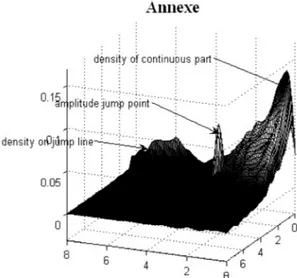
h n . The kernel estimate function is presented by figure 1 in the annexe.
From this figure, we note that there are a jump point localized in the block [1, 2] [3.5,4.5] and a jump line passing through points (0,7) and (1,6) . Then we propose for its joint probability measure the following model:
1 ( 11 21, ) ( , )
= ( , ) ( ) u au b .
d f x y dxdy a u
The jump point: (w w11, 21) is localized in the block [1, 2] [3.5,4.5] . From the
fact that (0,7) and (1,6) are belonging to the jump line, it is easy to see that the equation of the jump line is: =y . In order to calculate the estimators x 7
ˆ( , )
f x y , ˆ ( , )a x yn and ˆ( , )x y , defined in the section 2, we must choose the
spectral windows.This amounts to choose W , (1) W , (2) W and (3) W satisfying: (4)
(1) (1) (2) (2) (1) (1) 1 1 ( n ) = ( n ) , n n W M x W M x x M M (3) (1) (4) (2) (1) (1) 1 1 ( n ) = ( n ) , n n W L x W L x x L L
To simplify, we take W(1)=W and (3) W(2)=W with (4) (1)= (1)
n n
M L and
(2)= (2)
n n
M L . Choosing Mn(1)=n and p Mn(2)=n with 0 < < < 3/5q q p ,
3/5
=
n n
. These parameters satisfy the hypothesis given in § 2.1 and § 2.2.
First, choosing W as a nonnegative, even and integrable function. We pro-(1)
pose: (1) 64 64 if [ 1, 1/8[ 63 63 8/9 if [ 1/8,1/8] ( ) = 64 64 if ]1/8,1] 63 63 0 otherwise t t t W t t t
It is easy to show that
W(1)( ) = 1t dt .Choosing now a nonnegative, even and integrable function W such that (2) (1)
W and W satisfying (3). We propose: (2)
(1) (1) (2) (2) (2) (1) if [ 1/8,1/8] ( ) = 4/7 1 if [ 1, 1/8[ ]1/8,1] 0 otherwise n n n M W t t M M W t t M
1/8 1/8 1 (2) (2) (2) (2) 1 1/8 1/8 ( ) = ( ) ( ) ( ). W t dt W t dt W t dt W t dt
(2) 1/8 (2) (2) (1) 1/8 ( ) = 1 Mn ( ) W t dt W t dt M
. From the definition of W , we (2)have (1) 1/8 (2) 1/8 (1) (2) 1/8 ( ) = 2 0 n n M W t dt W t dt M
. Putting = n(1)(2) n M u t M , we have (1) 1/8 (2) (2) 1/8 (2) (1) (1) 1/8 ( ) = 2 0 ( ) . Mn M n n n M W t dt W u du M
Since n(1)(2) n MM , for n large enough we have (1) (2) > 1 n n M M . Thus, we obtain (2) 1/8 (2) 1 (1) (1) 1/8 ( ) = 2 0 ( ) . n n M W t dt W u du M
W being even and (1) W(1)( ) = 1t dt
, we deduce (2) 1/8 (2) (1) 1/8 ( ) = . n n M W t dt M
Thus,
W(2)( ) = 1t dt .Let us show that (3) is satisfied. Indeed, let t a real number belonging
to 1(1), 1(1) n n M M , since (2) (1) n n M
M converges to zero, for n large enough, we
have (2) (2) (2) (1) (1) 1/8 < n n < 1/8 n n n M M M t M M
. Therefore, from (16), we have:
(1) (2) (2) (1) (2) (1) (1) (2) ( ) = n = ( ). n n n n M W M t W M t W M t M
The graphic (fig 2) of the estimate ˆ( , )f x y defined in the section 2 is given in the
annexe.
6.1 Statistical Tests
After several attempts testing points in the block [1, 2] [3.5,4.5] , we found a jump at the point: ( , ) = (1.5,4)x y . Indeed, we calculate L defined in § 4.1, we obtain: 1/2 2 2 2 1/2 1 2 1 2 ˆ ( , ) = ˆ = 3.954 ( (0,0) ( , ) ( , ) ) n a x y n L K f x y K t t dt dt
read the value: Z/2=1.96. Since L [ Z/2,Z/2], we conclude that (1.5,4) is
a jump point.
For any other point the test concludes that it is not significantly a jump point. To illustrate this, taking, for example, ( , ) = (2,4)x y . Calculation of L at ( , ) = (2,4)x y gives L= 0.012. Since L [ Z/2,Z/2], we conclude that (2,4)
is not a jump point. 7. CONCLUSIONS
We have presented in this paper some results about limits theorems of density estimate when the measure has certain mixture. A statistical test for detecting the jump point is given and applied to study the humidity and resistance of agricul-tural soil. this work could be applied to other cases when the distribution contains points of discontinuity that risks being badly treated by sharing interval distribu-tion or by using Monte Carlo method. The proposed methods can be extended to other applications in several sectors. Indeed, the control of the quality for a prod-uct manufactured in the auto industry use the measure of two variables: the sumption of diesel and the pollution. Their joint distribution can follow a con-tinuous law except some observations which are taken when there is fog and reached the constant value (point of the jump). One example in economics, it is the observation of the variables: taxes on income and purchasing power can have a joint distribution contains some point of jumps due to exemption (disabled, former soldier, ...). In oceanography when we observe, by using a camera placed at a certain depth in water, two variables: the length of the fishes and their movement speed. The joint distribution may represent some jumps due to the acceleration of movement during the passage of a predator. In Astronomy the repeated passage of an object preventing the vision of stars (cloud, bird, ...) can create a jump of data. This work could be supplemented by the study of optimal smoothing parameters using cross validation techniques that have proven in this field.
Figure 1 – The kernel density of bivariate random variable (X,Y ).
Figure 2 – The density estimate ˆf x y . ( , )
Agrosup Dijon/Université de Bourgogne RACHID SABRE
France
ACKNOWLEDGMENTS
I would like to thank the anonymous referees for their interest in this paper and their valuable comments and suggestions.
REFERENCES
M. BERTRAND-RETALI, (1978), Convergence d’un estimateur de la densité par la méthode du noyau, Re-vue Roumaine de Mathématiques pures et Appliquées. T XXIIII, N 3, 361-385. P. BILLINGSLEY, (1968) Convergence of probability measures, Ed. Willey, New York. D. BOSQ , J.P. LECOUTRE, (1987) Théorie de l'estimation fonctionnelle, Ed. Economica, Paris. A. W. BOWMAN, P. HALL and D. M. TITTRINGTON, (1984), Cross-validation in nonparametric estimation
of probabilities and probability density, Biometrika, 71, 341-352.
L. DEVROYE, (1987), A course in density estimation, Ed. Birkhauser.
J. FAN, (1991), On the optimal rates of convergence for nonparametric deconvolution problems, Annals of Statistics., 19, 1257-1272.
E. PARZEN, (1962), On the estimation of a probability density function and mode, The Annals of Mathematics Statistics, 33, 1065-1076.
M. ROSEMBLATT, (1965), Remarks on some nonparametric estimates of a density function, The Annals of Mathematics Statistics, 27, 832-837.
M. RACHDI, R. SABRE, (2000), Consistent estimates of the mode of the probability density function in
non-parametric deconvolution problems. Statistics & Probability Letters, 47(2000), 105-114.
65-78.
R. SABRE, (1994), Estimation de la densité de la mesure spectrale mixte pour un processus symétrique
stable strictement stationaire, Comptes Rendus de l’Académie des Sciences à Paris, t. 319,
Série I, p. 1307-1310.
R. SABRE, (1995), Spectral density estimation for stationary stable random fields, Applicationes Mathematicae, 23, 2, p. 107-133.
R. SABRE, (2003), Nonparametric estimation of the continuous part of mixed measure, Revisita Statis-tica, vol. LXIII, n. 3, pp. 441-467.
A. STEFANSKI, (1990), Rates of convergence of some estimators in a class of deconvolution problems, Sta-tistics & Probability Letters, 9, p. 229-235.
P. VIEU, (1996), A note on density mode estimation, Statistics & Probability Letters, 26, p. 297-307.
C.H. ZHANG, (1990), Fourier methods for estimating mixing densities and distributions, Annals of Statistics, 18, p. 806-830.
SUMMARY
Test and asymptotic normality for mixed bivariate measure
Consider a pair of random variables whose joint probability measure is the sum of an absolutely continuous measure, a discrete measure and a finite number of absolutely con-tinuous measures on some lines called jum lines. The central limit theorem of the densi-ties estimates is studied and its rate of convergence is given. A statistical test is developed to locate the jump points. An application on real data was conducted.