Apprendimento automatico delle relazioni fra documenti dal web

(1)

Learning relational models

from networked data on the web

Davide Riva

Master Thesis

Universit`a di Genova, DIBRIS Via Opera Pia, 13 16145 Genova, Italy https://www.dibris.unige.it/

(2)

MSc Computer Science

Data Science and Engineering Curriculum

Learning relational models

from networked data on the web

Davide Riva

Advisors: Annalisa Barla, Davide Garbarino

Examiner: Nicoletta Noceti

(3)

Abstract

Network inference is the process of uncovering relations between data, particularly effective in biology to reconstruct Gene Regulatory Networks (GRN). Supervised methods were also proposed in the past to model a network of documents and predict links between them. In this thesis, we propose an unsupervised approach to extract an undirected and un-weighted graph given a collection of texts. In particular, we present a pipeline to construct and use a dataset composed of pages of a given website.

(4)

I wish to express my deepest gratitude to all students and professors who went along with me on this journey. Among those, a special thanks to Eros Viola, Riccardo Bianchini, Olga Matthiopoulou, Marco Rando, Andrea Canepa, Larbi Touijer, Federico Lodovici, Roberto Castellotti, Antonio Vivace, Marco Orsingher, Michele Pugno, Adrian

Castro, Annalisa Barla, Nicoleta Noceti and Davide Garbarino.

In addition, I would like to thank Jordan Boyd-Graber and David M. Blei who released for free their lessons, talks and material which were useful during the writing of this

thesis.

I am also indebted to Fabio Antonio Stella, which made me fall in love with this subject and played an important role in the choices I made that led me here.

I wish to acknowledge the support and great love of Laura and her family, which helped me tackle this degree course which is going to end.

Last but not least, I would like to recognize the invaluable economic assistance that my family provided during my study.

(5)

Chapter 1 Introduction and motivation

In the field of biology, unsupervised methods like ARACNE (see [MNB+06]) are used to obtain Gene Regulatory Networks starting from microarray expression profiles.

Methods like Relational Topic Model (introduced in [CB09]) were also proposed to model a collection of documents and the links between them in a supervised way.

The goal of this thesis is to propose a novel approach to perform network inference given a collection of webpages scraped from a website, exploiting ideas from the two methods mentioned before. In particular, the final result is an unweighted and undirected graph which connects pages with similar content.

The manuscript is organized as follows: in Chapter 2 we present some techniques to en-code words numerically. In Chapter 3 we move from word to document representations and we describe Topic Modeling. In Chapter 4 we describe network inference, presenting ARACNE. Chapter 5 and Chapter 6 describe our original approach, outling some possi-ble future directions. Finally, Appendices A, B, C and D cover a part of the background knowledge required to read this document.

(8)

Chapter 2 Word Embedding

Documents are made by words. To be manipulable by an algorithm these words need to be represented in a numerical format.

This chapter covers some techniques able to fulfil this task, pointing out the advantages and disadvantages of choosing one instead of another.

To avoid misunderstandings we define the term “word” as a word in a particular position in a document, while we use the word “term” as a generic word into a dictionary.

For instance, given a document “A cat is an animal but an animal is not a cat” its list of words is 𝑤 = (𝑎, 𝑐𝑎𝑡, 𝑖𝑠, 𝑎𝑛, 𝑎𝑛𝑖𝑚𝑎𝑙, 𝑏𝑢𝑡, 𝑎𝑛, 𝑎𝑛𝑖𝑚𝑎𝑙, 𝑖𝑠, 𝑛𝑜𝑡, 𝑎, 𝑐𝑎𝑡) while its set of terms is 𝑑 = {𝑎, 𝑐𝑎𝑡, 𝑖𝑠, 𝑎𝑛, 𝑎𝑛𝑖𝑚𝑎𝑙, 𝑏𝑢𝑡, 𝑛𝑜𝑡}.

2.1 One Hot Encoding

Given a list of words 𝑤 = (𝑤1, 𝑤2, . . . , 𝑤𝑁), we first generate a dictionary of unique terms

𝑑 = {𝑑1, 𝑑2, ..., 𝑑𝐾} with an arbitrary order between words. Note that 𝐾 ≤ 𝑁 is always

true and 𝐾 = 𝑁 happens only when there is no repetition of words in the documents. Each term 𝑑𝑖 in the dictionary can now be encoded as 𝑥𝑖 ∈ {0, 1}𝐾 following the One Hot

Encoding approach. All elements of 𝑥𝑖 are zero except a “1” in the position 𝑖 of the vector.

That means that two words 𝑤𝑙, 𝑤𝑗 in different positions will have the same value 𝑥𝑖 if and

only if they correspond to the same term 𝑑𝑖.

Applying One Hot Encoding on the previous example presented in the introduction of this chapter leads to the following values of 𝑥𝑖:

(9)

• 𝑥1 = 𝑥𝑎= [1, 0, 0, 0, 0, 0, 0] • 𝑥2 = 𝑥𝑐𝑎𝑡= [0, 1, 0, 0, 0, 0, 0] • 𝑥3 = 𝑥𝑖𝑠= [0, 0, 1, 0, 0, 0, 0] • 𝑥4 = 𝑥𝑎𝑛 = [0, 0, 0, 1, 0, 0, 0] • 𝑥5 = 𝑥𝑎𝑛𝑖𝑚𝑎𝑙 = [0, 0, 0, 0, 1, 0, 0] • 𝑥6 = 𝑥𝑏𝑢𝑡 = [0, 0, 0, 0, 0, 1, 0] • 𝑥7 = 𝑥𝑛𝑜𝑡 = [0, 0, 0, 0, 0, 0, 1]

Despite its simplicity and the fact that it is not computationally expensive to use, it has some disadvantages:

• vectors are sparse: only one element of each vector is not zero

• there is no concept of similarity: all vectors have the same distance between each other

2.2 Word2vec

Word2vec is a family of approaches to overcome the disadvantages of One Hot Encoding using neural networks. Originally presented in [MCCD13], it was later resumed by other authors due to the lack of details in the original paper. For our document, we use [Ron14] as a reference.

In this section, two architectures are proposed. Both of them should be trained using mini-batch gradient descent instead of gradient descent to allow the algorithm to scale when datasets grow in size.

After a learning phase, they will be able to map each term 𝑥𝑖 ∈ {0, 1}𝐾 to a point 𝑦𝑖 ∈ R𝑉,

with 𝑉 ≪ 𝐾. Points in the new space will have a notion of similarity: if two terms 𝑑𝑙 and

𝑑𝑗 appear in similar contexts and/or they have the same semantic content, their vectors

𝑦𝑙 and 𝑦𝑗 will be close together. On the opposite situation, 𝑦𝑙 and 𝑦𝑗 will be distant from

each other.

For instance, 𝑦𝑐𝑎𝑡 will probably be closer to 𝑦𝑑𝑜𝑔 than 𝑦𝑐𝑜𝑚𝑝𝑢𝑡𝑒𝑟.

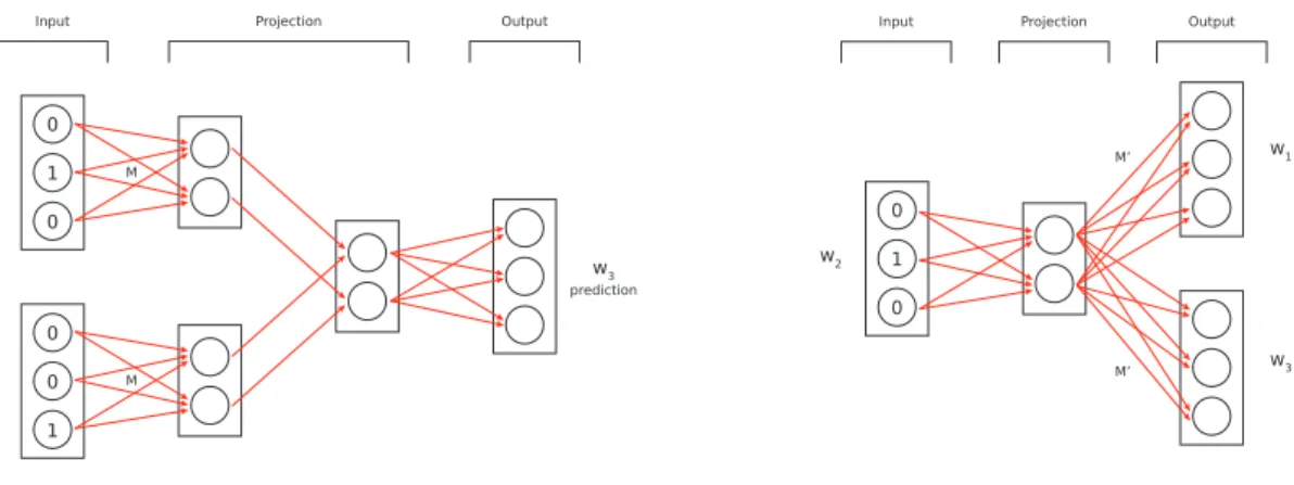
2.2.1 Continuous Bag-of-Words Model (CBOW)

First, the entire corpus is divided into contiguous blocks of words with odd length 𝑁 called n-grams.

Suppose to have the phrase “A cat is the best animal.” and n-grams of size 3. The corresponding blocks are:

(10)

1 0 0 0 0 1 w4 w3 w3 prediction M M

Input Projection Output

1 0 0 w2 w1 w3 M’ M’

Input Projection Output

Figure 2.1: CBOW (left) and Skip-Gram (right) models with 𝐾 = 3 and 𝑉 = 2.

• (𝑎, 𝑐𝑎𝑡, 𝑖𝑠) • (𝑐𝑎𝑡, 𝑖𝑠, 𝑡ℎ𝑒)

• (𝑖𝑠, 𝑡ℎ𝑒, 𝑏𝑒𝑠𝑡) • (𝑡ℎ𝑒, 𝑏𝑒𝑠𝑡, 𝑎𝑛𝑖𝑚𝑎𝑙)

The goal is to predict a word given its context. For each n-gram, the CBOW neural network has as inputs all words in the block except the one in the center which is used as ground truth for the classification task. All words are encoded using the One Hot Encoding method.

For each n-gram, the first layer takes each input word encoded as 𝑥𝑖 ∈ {0, 1}𝐾 and projects

it into a smaller space R𝑉 _{where 𝑉 is a hyperparameter to tune. This is done through}

a shared matrix 𝑀𝐾×𝑉 which represents a fully connected layer. Each projection is then

averaged out with the others in the same block. Note that in this way the order of the input words of the same sequence does not matter anymore.

The previous layer is then linked to a final layer in a fully connected way. Since the classification task is on a One Hot Encoding vector, a softmax activation function is used at the end.

Instead of using the network for the task for which it was trained, we use the matrix 𝑀𝐾×𝑉

to encode all terms as vectors in R𝑉_.

Note that there is no need to compute 𝑀 𝑥𝑖 for each 𝑖. Since every 𝑥𝑖 has zero values

everywhere except a “1” in the position 𝑖 of the vector, the result of the multiplication 𝑀 𝑥𝑖 is the 𝑖-th row 𝑖 the matrix M. For this reason, each row 𝑖 of 𝑀 represents the term

(11)

An illustration of CBOW can be seen in Figure 2.1.

2.2.2 Continuous Skip-gram Model (Skip-gram)

The Skip-gram model is the opposite approach of CBOW.

For each n-gram, the word in the center is fed to the neural network as the only input. The second layer projects it to a smaller space through a matrix 𝑀𝐾×𝑉. Unlike the previous

model, there is no averaging since there is just one word as input.

Finally, the last layer tries to predict all remaining words of a block. Each predicted word is obtained multiplying the hidden layer with a shared matrix 𝑀_{𝑉 ×𝐾}′ . For each group of 𝐾 nodes which refers to a predicted word, we apply separately a softmax function. To increase the accuracy, we can pick the number of output words less than 𝑁 − 1 and then sampling words in the same phrase weighted by how distant they are from the input word. If there are 𝑁 − 1 words to predict and each word is represented as a vector in R𝐾_{, the}

total number of nodes of the final layer is (𝑁 − 1)𝐾.

As previously, we use the matrix 𝑀 to encode each term 𝑥𝑖.

An illustration of Skip-Gram can be seen in Figure 2.1.

2.2.3 Interpretation of the results

CBOW and Skip-Gram models are similar to Autoencoders, with the difference that we are using the intermediate representations to predict words in the same phrase. This leads to words having close values of 𝑦 if they appear often in the same context.

Furthermore, the paper [MCCD13] found out that these models go beyond syntactic reg-ularities: for example, the result of 𝑦𝑘𝑖𝑛𝑔 − 𝑦𝑚𝑎𝑛+ 𝑦𝑤𝑜𝑚𝑎𝑛 is the closest vector to 𝑦𝑞𝑢𝑒𝑒𝑛.

Note that subsequent papers like [NvNvdG19] scale down the previous claim, adding the constraint that no input vector can be returned by the prediction.

2.3 Global Vectors (GloVe)

GloVe was proposed in [PSM14] to overcome the limitations of Word2vec. In particular, it builds a term-term co-occurrence matrix to utilize the statistics of the entire corpus instead of training the model on single n-grams.

(12)

Let 𝑋 the term-term co-occurrence matrix. 𝑋𝑖𝑗 measures how many times the term 𝑑𝑖

occurs in the corpus near the term 𝑑𝑗. Based on how you define the term “near”, the

elements of the matrix will have different values. For simplicity, we increment the counter (𝑋𝑖𝑗 = 𝑋𝑖𝑗 + 1) every time two terms appear in a phrase with less than 𝑁 words between

them, with 𝑁 a hyperparameter to tune. Given that, 𝑋 is symmetric. An initial proposal could be to solve min𝑢,𝑣

∑︀

𝑖,𝑗(𝑢𝑇𝑖 𝑣𝑗 − 𝑋𝑖𝑗)2 in order to have vectors

𝑢𝑖, 𝑣𝑗 ∈ R𝑉 that have a high dot product if the terms 𝑑𝑖 and 𝑑𝑗 appear frequently together

and vice versa.

We then apply the logarithm to 𝑋𝑖𝑗:

min

𝑢,𝑣

∑︁

𝑖,𝑗

(𝑢𝑇_𝑖 𝑣𝑗 − 𝑙𝑜𝑔2(𝑋𝑖𝑗))2

In this way, we lower the gap between frequent terms and rare ones.

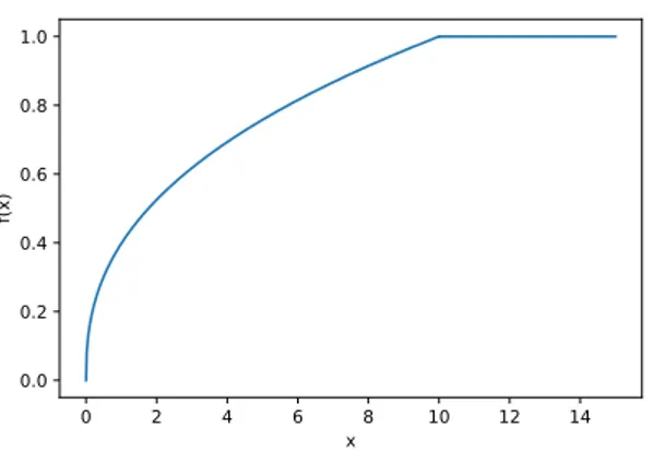
The huge problem with this model is that all terms are weighted in the same way, no matter how frequent they appear in the corpus. To avoid this drawback, we introduce a weighting function 𝑓 (𝑋𝑖𝑗) with the following characteristics:

• 𝑓(0) = 0: when 𝑋𝑖𝑗 = 0 the previous equation is undefined, while here the

co-occurrence is not considered

• 𝑓 should be non-decreasing: frequent terms must be considered more than rare ones

• 𝑓 needs to have a cutoff to avoid weighting too much terms that appear often in the text and which do not convey semantic information. These terms are commonly called “stop words” in the literature. Examples are “the”, “a”, “from” and so on. An illustration of a valid 𝑓 (𝑋𝑖𝑗) can be viewed in Picture 2.2.

After this addition, the minimization problem becomes: min

𝑢,𝑣

∑︁

𝑖,𝑗

𝑓 (𝑋𝑖𝑗)[𝑢𝑇𝑖 𝑣𝑗− log2(𝑋𝑖𝑗)]2

Consider that even the summation is over all combinations of terms, the matrix is sparse and so the minimization is not as computationally intensive as computing it on a dense matrix.

After taking gradient descent to resolve that minimization, we will obtain vectors 𝑢𝑗, 𝑣𝑗

similar between each other because of the symmetricity of 𝑋. Since 𝑢𝑗 ≃ 𝑣𝑗, a reasonable

choice for our new vector representation of each term 𝑑𝑗 could be taking their average:

𝑦𝑗 =

𝑢𝑗 + 𝑣𝑗

(13)

0 2 4 6 8 10 12 14 x 0.0 0.2 0.4 0.6 0.8 1.0 f( x)

Figure 2.2: Example of a valid 𝑓 (𝑋𝑖𝑗) function for the minimization step of GloVe.

2.4 Measuring distances between terms

In the previous sections the term “close” was intentionally left vague. Different distances between vectors could be considered. In particular, we propose two of them:

• euclidian distance: distance(𝑝, 𝑞) = √︀∑︀𝑖(𝑝𝑖− 𝑞𝑖)2

• cosine similarity: distance(𝑝, 𝑞) = 𝑝𝑇_𝑞

‖𝑝‖‖𝑞‖ = ∑︀ 𝑖𝑝𝑖𝑞𝑖 √ ∑︀ 𝑖𝑝2𝑖 √ ∑︀ 𝑖𝑞2𝑖

While the first one measures the straight-line distance of two points, the second one returns the cosine of the angle between the corresponding vectors.

In the literature presented, the cosine similarity is the default choice to measure the close-ness between terms. One reason to prefer it instead of the euclidian distance can be found in [SW15]: the magnitude of the vector representation of a term is correlated with the fre-quency of its appearance in the corpus which means that a term with the same semantical meaning of another could have a different magnitude if it appears more often in text than the other one.

(14)

Chapter 3 Topic Modeling

In Chapter 2, we presented some techniques to encode words as vectors. Starting from a Bag-of-Words model in which we assume that the order of the words inside a text does not matter, it is possible to follow a similar approach also for documents. Topic models play an important role in describing, organizing and comparing unstructured collections of documents.

The first step is to generate a matrix of term counts 𝑋 for the entire corpus: each row is a document represented in the BOW format and each column represents the count of occurrence of a particular term in the documents.

The goal of the second step is to produce two matrices:

• term-topic matrix: each row represents how related each term is to all topics • document-topic matrix: each row represents how related each document is to all

topics

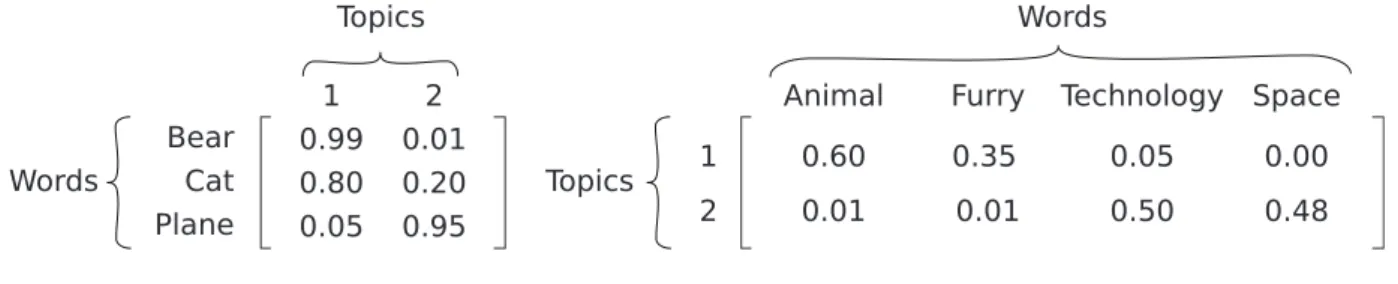
For instance, a document about bears is likely to have high intensity on some topics which in turn have high intensity on words related to animals; see Figure 3.2 for an example.

3.1 Latent Semantic Analysis (LSA)

Given the number of topics 𝑉 as an hyperparameter, Truncated SVD is applied to the matrix obtained in the first step (see Figure 3.1 for a graphical representation):

𝑋𝑁 ×𝐾 = 𝑈𝑁 ×𝑉Σ𝑉 ×𝑉𝐷𝐾×𝑉𝑇

(15)

matrix.

Using 𝑈 instead of 𝑋 for comparing documents when 𝑉 ≪ 𝐾 leads to a smaller memory footprint. Furthermore, the terms are no longer orthogonal: thanks to this it is possible to compute the similarity between a term and a document even if the document does not contain the term itself. The key point to observe is that both terms and documents are described as topics: if a term is frequent in some topics and a document is frequent in the same topics, they will have a similar representation in the new space.

An overview of this technique can be found at [Dum04].

X

≃

U Σ V

Figure 3.1: Truncated SVD represented graphically; matrices size proportions are kept intact Words Bear Cat 0.99 Topics 0.80 0.05 0.01 0.20 0.95 1 2 0.60 0.01 0.05 0.01 0.35 0.50 0.00 0.48 Plane

Animal Furry Technology Space

Topics 1

2

Words

Figure 3.2: Example of a term-topic and a document-topic matrix.

3.2 Latent Dirichlet Allocation (LDA)

LDA makes the same assumptions about topics as LSA but unlike the latter, it views topics and documents in a probabilistic way. In particular, a document is a categorical distribution over topics 𝜃𝑑 and a topic is a categorical distribution over words 𝛽𝑖. The

probability of sampling a document is instead modelled as a Dirichlet distribution 𝐷𝑖𝑟(𝛼). A major drawback of LDA is that the number of topics is assumed to be known a-priori and treated as a hyperparameter.

(16)

Variants of this model are present in the literature: in this chapter, we use [Ble11] and [BNJ03] as a reference.

3.2.1 Generative process

In this section we describe LDA by its generative process, assuming we have already ob-tained the parameters of the model.

We define:

• 𝛽1:𝐾: 𝐾 topics, where each topic 𝛽𝑖 is a distribution over the terms in the vocabulary

• 𝜃𝑑: a document 𝑑 described as a categorical distribution over topics, where 𝜃𝑑,𝑘 is

the topic proportion for topic 𝑘 in document 𝑑

• 𝑤𝑑: observed words of document 𝑑, where 𝑤𝑑,𝑛 is the word in position 𝑛 of document

𝑑

The generation of 𝑀 documents with 𝑁 words each can be summarized as: 1. 𝜃𝑑∼ 𝐷𝑖𝑟(𝛼): pick a document

2. 𝑧𝑑,𝑛 ∼ Mult (𝜃𝑑): sample a topic

3. 𝑤𝑑,𝑛 ∼ 𝛽𝑧𝑑,𝑛: pick a term

4. use that term as a word for the document you want to generate 5. loop 𝑁 times to step 2

6. loop 𝑀 times to step 1

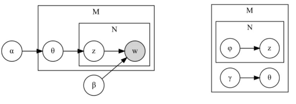
LDA is a probabilistic graphical model and it is represented graphically in Figure 3.3. The joint distribution is:

Given the distributions explained before, we can state that:

𝑝(𝜃𝑑|𝛼) = 1 𝐵(𝛼) 𝐾 ∏︁ 𝑘=1 𝜃𝛼𝑘−1 𝑑,𝑘 𝑝(𝑧𝑑,𝑛|𝜃𝑑) = 𝜃𝑑,𝑧𝑑,𝑛 𝑝(𝑤𝑑,𝑛|𝑧𝑑,𝑛, 𝛽) = 𝛽𝑧𝑑,𝑛,𝑤𝑑,𝑛

(17)

M N α θ β w z M N θ γ φ z

Figure 3.3: Graphical model representation of LDA (left) and graphical model representa-tion of the variarepresenta-tional distriburepresenta-tion (right). Nodes are random variables, shaded if observed. An edge denotes a dependence between two random variables. Plates denote multiplicity.

3.2.2 Model inference

The goal of LDA is to automatically discover topics over a collection of documents. Since only words are observed, topics are considered latent variables.

Note that inference in this case can be seen as the reverse of the generative process explained in Section 3.2.1.

Mathematically speaking, inference becomes a question of computing the posterior distri-bution:

𝑝(𝜃, 𝑧|𝑤, 𝛼, 𝛽) = 𝑝(𝜃, 𝑧, 𝑤|𝛼, 𝛽) 𝑝(𝑤|𝛼, 𝛽)

The denominator 𝑝(𝑤1:𝐷|𝛼, 𝛽) is the probability of observing the corpus under all possible

topic model combinations and thus intractable to compute. For this reason, in this section we approximate the posterior distribution through a variational method (see Appendix D). In particular, we set 𝑞 as:

𝑞(𝜃𝑑|𝛾𝑑) is governed by a Dirichlet distribution, while 𝑞(𝑧𝑑,𝑛|𝜑𝑑,𝑛) by a Categorical

(18)

To do model inference from a collection of documents, we start defining the ELBO function: ln[∏︁ 𝑑 𝑝𝑑(𝑤|𝛼, 𝛽)] ≥ E 𝑞{ln[𝑝(𝑤, 𝜃, 𝑧|𝛼, 𝛽)] − ln[𝑞(𝜃, 𝑧|𝛾, 𝜑)]} = E 𝑞{ln[ ∏︁ 𝑑 𝑝𝑑(𝑤, 𝜃, 𝑧|𝛼, 𝛽)] − ln[ ∏︁ 𝑑 𝑞𝑞(𝜃, 𝑧|𝛾, 𝜑)]} = E 𝑞{ ∑︁ 𝑑 ln[𝑝𝑑(𝑤, 𝜃, 𝑧|𝛼, 𝛽)] − ∑︁ 𝑑 ln[𝑞𝑞(𝜃, 𝑧|𝛾, 𝜑)]} =∑︁ 𝑑 E 𝑞{ln[𝑝𝑑(𝑤, 𝜃, 𝑧|𝛼, 𝛽)] − ln[𝑞𝑞(𝜃, 𝑧|𝛾, 𝜑)]} =∑︁ 𝑑 E 𝑞𝑑 {ln[𝑝𝑑(𝑤, 𝜃, 𝑧|𝛼, 𝛽)] − ln[𝑞𝑑(𝜃, 𝑧|𝛾, 𝜑)]}

First, we fix 𝛼 and 𝛽 to find the best 𝑞(𝜃, 𝑧|𝛾, 𝜑) that minimizes the KL-divergence between 𝑞 and 𝑝. Then, we fix (𝜃, 𝑧|𝛾, 𝜑) to find the best 𝛼 and 𝛽 that maximize the lower bound. This process, if done iteratively, converges to a local optimum. In the literature, it is called expectation-maximization (EM).

Since constrained maximization and the Newton-Raphson algorithm are needed to solve the problem instead of traditional variational inference, we intentionally present only a hasty description of the update algorithm:

1. initialize 𝛽 randomly, set each 𝜑𝑑,𝑛 as _𝐾1 and each 𝛾𝑑 as 𝛼𝑑+𝑁_𝐾

2. for each document, update the local latent variables 𝛾 and 𝜑 until convergence 3. update the global variables 𝛽 and 𝛼 for the entire corpus until convergence 4. loop to 2 until convergence

The updates are affected by: • 𝜑𝑑,𝑛,𝑘 ∝ 𝛽𝑘,𝑤𝑛𝑒

Ψ(𝛾𝑑,𝑘)−∑︀𝐾𝑗 Ψ(𝛾𝑑,𝑗)_{, where Ψ is the first derivative of the logarithm of the}

gamma function • 𝛾𝑑,𝑘 = 𝛼𝑘+ ∑︀ 𝑛𝜑𝑑,𝑛,𝑘 • 𝛽𝑘,𝑗 ∝∑︀_𝑑∑︀_𝑛1[𝑤𝑑,𝑛==𝑗]𝜑𝑑,𝑛,𝑘 • 𝜕ELBO 𝜕𝛼𝑘 = ∑︀ 𝑑[Ψ( ∑︀𝐾 𝑗 𝛼𝑗) − Ψ(𝛼𝑘) + Ψ(𝛾𝑑,𝑘) − Ψ( ∑︀𝐾 𝑗 𝛾𝑑,𝑗)]

The interested reader can find more details looking at Appendix A of [BNJ03].

Note that step 2 can be parallelized: each document has its local variables that are condi-tionally independent of the other local variables and data in different documents.

(19)

After the execution of the algorithm, each row 𝑑 of the final document-topic matrix can be obtained using the Maximum Likelihood Estimation method over 𝑞(𝜃𝑑|𝛾𝑑).

3.2.3 Sparsity considerations

Using the Dirichlet governed by the 𝛼 parameter to induce sparsity allows us to have doc-uments described by fewer topics than using an uninformative prior. The same reasoning can be applied to topics, introducing a Dirichlet that governs the probability of having a topic with a particular set of terms.

Inducing sparsity combined with the number of topics much less than the number of docu-ments lower the risk of obtaining two different topics with a similar distribution of words.

3.3 Online LDA

A major drawback of LDA is the impossibility to scale as the data grows: each iteration of the algorithm requires an entire scan of the corpus, which is computationally expensive. For this reason, [HBB10] proposes an online learning variation based on the original LDA model. This algorithm called online LDA does not need to store all documents together, but they can arrive in a stream and be discarded after one look.

The main difference between the graphical model presented in Section 3.2.2 and this one is that the latter assumes each 𝛽𝑘 sampled from a Dirichlet distribution as presented in

Section 3.2.3:

𝛽𝑘 ∼ 𝐷𝑖𝑟(𝜂) (3.1)

For this reason, 𝑞 becomes:

𝑞(𝛽, 𝜃, 𝑧|𝜆, 𝛾, 𝜑) = [∏︁ 𝑘 𝑞𝑘(𝛽|𝜆)][ ∏︁ 𝑑 𝑞𝑑(𝜃, 𝑧|𝛾, 𝜑)] = [∏︁ 𝑘 𝑞(𝛽𝑘|𝜆𝑘)][ ∏︁ 𝑑 𝑞𝑑(𝜃|𝛾)𝑞𝑑(𝑧|𝜑)] = [∏︁ 𝑘 𝑞(𝛽𝑘|𝜆𝑘)]{ ∏︁ 𝑑 [𝑞(𝜃𝑑|𝛾𝑑) ∏︁ 𝑛 𝑞(𝑧𝑑,𝑛|𝜑𝑑,𝑛)]}

𝑞(𝛽𝑘|𝜆𝑘) and 𝑞(𝜃𝑑|𝛾𝑑) are governed by a Dirichlet distribution, while 𝑞(𝑧𝑑,𝑛|𝜑𝑑,𝑛) by a

Cat-egorical distribution.

Due to that change compared to LDA, the ELBO is now:

ln[𝑝(𝑤|𝛼, 𝜂)] ≥ E

(20)

If we have 𝑀 documents, the ELBO can be factorized as: { 𝑀 ∑︁ 𝑑=1 E 𝑞[ln 𝑝𝑑(𝑤|𝜃, 𝑧, 𝛽) + ln 𝑝𝑑(𝑧|𝜃) − ln 𝑞𝑑(𝑧|𝜑) + ln 𝑝𝑑(𝜃|𝛼) − ln 𝑞𝑑(𝜃|𝛾)]} + E 𝑞[ln 𝑝(𝛽|𝜂) − ln 𝑞(𝛽|𝜆)] = { 𝑀 ∑︁ 𝑑=1 E 𝑞[ln 𝑝𝑑(𝑤|𝜃, 𝑧, 𝛽) + ln 𝑝𝑑(𝑧|𝜃) − ln 𝑞𝑑(𝑧|𝜑) + ln 𝑝𝑑(𝜃|𝛼) − ln 𝑞𝑑(𝜃|𝛾)] + [ln 𝑝(𝛽|𝜂) − ln 𝑞(𝛽|𝜆)]/𝑀 }

Similar to what we do for LDA, we could maximize the lower bound using coordinate ascent over the variational parameters. As for LDA, it requires a full pass through the entire corpus at each iteration.

To fix this issue, we load documents in batches. For each batch 𝑡 of size 𝑆, we compute the local parameters 𝜑𝑡 and 𝛾𝑡, holding 𝜆 fixed. Then, we compute an estimate of 𝜆 related to

that batch that we call ˜𝜆𝑡 and we update 𝜆 as a weighted average between its earlier value

and ˜𝜆𝑡:

𝜆 = (1 − 𝜌𝑡)𝜆 + 𝜌𝑡𝜆˜𝑡, 𝜌𝑡= (𝜏0+ 𝑡)−𝑠

where 𝜌𝑡 controls the importance of old values given the new ones. In particular:

• increasing the value of 𝜏0 ≥ 0 slows down the initial updates

• 𝑠 ∈ (0.5, 1] controls the rate at which old information is forgotten We can also incorporate updates of 𝛼 and 𝜂:

• 𝛼 = 𝛼 − 𝜌𝑡𝛼˜𝑡

• 𝜂 = 𝜂 − 𝜌𝑡𝜂˜𝑡

The updates are affected by:

• ˜𝛼𝑡= [Hess−1(𝑙)][∇𝛼𝑙], where l is the sum of the ELBO of each document of the batch

• ˜𝜂𝑡= [Hess−1(𝑙)][∇𝜂𝑙] • 𝜑𝑑,𝑛,𝑘 ∝ 𝑒E𝑞[ln 𝜃𝑑,𝑘]+E𝑞[ln 𝛽𝑘,𝑤𝑛] • 𝛾𝑑,𝑘 = 𝛼𝑘+ ∑︀ 𝑛𝜑𝑑,𝑛,𝑘 • ˜𝜆𝑡,𝑘,𝑛 = 𝜂𝑘+ _|𝑆|𝐷 ∑︀(𝑡+1)𝑆−1_{𝑑=𝑡·𝑆} 𝜑𝑑,𝑛,𝑘

(21)

Note that if the batch size |𝑆| is equal to one, the algorithm becomes online.

After the execution of the algorithm, each row 𝑑 of the final document-topic matrix can be obtained using the Maximum Likelihood Estimation method over 𝑞(𝜃𝑑|𝛾𝑑). The same

reasoning can be applied for topics, using MLE over 𝑞(𝛽𝑘|𝜆𝑘).

3.4 Hierarchical Dirichlet process (HDP)

HDP was proposed in [WPB11] as a way to overcome the problem of choosing the number of topics in LDA and derived methods while using an online variational inference algorithm. In particular, the number of topics is inferred from data.

Since this method uses the Dirichlet process, we need to introduce it first.

3.4.1 Dirichlet process (DP)

The Dirichlet process can be used as a generalization of the Dirichlet distribution which does not have a fixed number of topics.

Formally, it is defined as a two parameter distribution DP (𝛼, 𝐻), where 𝛼 is the concen-tration parameter and H is the base distribution.

To get an intuition on how it works, it can be viewed as a black-box which takes as input a continuous distribution 𝐻 and produces a discrete distribution 𝐺0 whose similarity with

𝐻 is governed by 𝛼: as 𝛼 → ∞, 𝐺0 = 𝐻.

The procedure of generating 𝐺0 can be described through the stick-breaking process. The

basic idea is that you have a stick of unit length and you break it off. At each iteration 𝑖, you pick the remaining part of the stick and you break it off again and again. The entire process takes an infinite number of steps since you can always break off the remaining part of a stick, ending up to smaller and smaller pieces.

More formally: 𝛽_𝑘′ ∼ Beta(1, 𝛼) 𝛽𝑘 = 𝛽𝑘′ 𝑘−1 ∏︁ 𝑙=1 (1 − 𝛽_𝑙′)

where 𝛽_𝑘′ is the percentage of the remaining stick that is break off and 𝛽𝑘 is the size of the

broken part of the stick after step 𝑘. All 𝛽𝑘 are then used as weights:

(22)

𝐺(𝑥) = ∞ ∑︁ 𝑘=1 1[𝑥==𝜑𝑘]𝛽𝑘

3.4.2 HDP nesting DPs

Using HDP instead of LDA or Online LDA requires the definition of a new model. First, we will describe the generative process. Then, we will analyse the steps of model inference.

3.4.2.1 Generative process

The model is composed of two layers:

• 𝐺𝑑|𝐺0 ∼ DP (𝛼, 𝐺0): each document 𝑑 is described by its own DP 𝐺𝑑

• 𝐺0 ∼ DP (𝛾, 𝐻): each 𝐺𝑑 is sampled from another DP 𝐺0; in this way all 𝐺𝑑 have

the same atoms and they differ only in their weights

where 𝐻 is a symmetric Dirichlet distribution over the vocabulary.

The stick-breaking construction of 𝐺0 is the same as the one presented in Section 3.4.1.

The one for each 𝐺𝑑 is instead:

• 𝑐𝑑,𝑘 ∼ Mult (𝛽) • 𝜋′ 𝑑,𝑘 ∼ Beta(1 , 𝛼) • 𝜋𝑑,𝑘 = 𝜋𝑑,𝑘′ ∏︀𝑘−1 𝑙=1(1 − 𝜋 ′ 𝑑,𝑙) • 𝐺𝑗(𝑥) = ∑︀∞ 𝑘=11[𝑥==𝜑_{𝑐𝑑,𝑘}]𝜋𝑑,𝑘

The generation of a word in position 𝑛 is then: • 𝑧𝑑,𝑛 ∼ Mult (𝜋𝑑)

• 𝜃𝑑,𝑛 = 𝜑𝑐_{𝑑,𝑧𝑑,𝑛}

• 𝑤𝑑,𝑛 ∼ Mult (𝜃𝑑,𝑛)

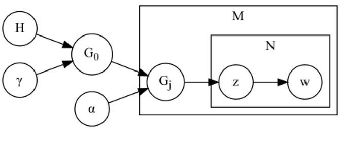
The plate notation of HDP is represented in Figure 3.4.

3.4.2.2 Model inference

Due to the fact that this process requires an infinite number of steps, truncation is needed to view the generative process and the inference as algorithms. In particular, we set a

(23)

M N H G₀ γ Gj α z w

Figure 3.4: Graphical model representation of HDP.

maximum number of global topics 𝐾 and a maximum number of local topics 𝑇 . Note that a reasonable choice is to set 𝑇 ≪ 𝐾 since the number of topics needed for a single document is less than the number of topics required for the full corpus.

Our variational distribution is:

• 𝑞(𝑐|𝜙) = ∏︀𝑑 ∏︀𝑇 𝑡=1𝑞(𝑐𝑑,𝑡|𝜙𝑑,𝑡) • 𝑞(𝑧|𝜁) = ∏︀𝑑 ∏︀ 𝑛𝑞(𝑧𝑑,𝑛|𝜁𝑑,𝑛) • 𝑞(𝜑|𝜆) = ∏︀𝐾 𝑘=1𝑞(𝜑𝑘|𝜆𝑘) • 𝑞(𝛽′_{|𝑢, 𝑣) =} ∏︀𝐾−1 𝑘=1 𝑞(𝛽 ′ 𝑘|𝑢𝑘, 𝑣𝑘) • 𝑞(𝜋′_{|𝑎, 𝑏) =}∏︀ 𝑑 ∏︀𝑇 −1 𝑡=1 𝑞(𝜋 ′ 𝑑,𝑡|𝑎𝑑,𝑡, 𝑏𝑑,𝑡) where 𝑞(𝛽_𝐾′ = 1) = 1 and ∀𝑑 𝑞(𝜋_𝑑,𝑇′ = 1) = 1.

As we did for LDA and Online LDA we take derivatives of the ELBO with respect to each variational parameter. The results are both document-level updates obtained using coordinate ascent and corpus-level updates computed using gradient ascent. These updates can be performed in an online fashion, computing local updates only for a small part of documents for each iteration and then performing the corpus-level updates using a noisy estimation of the gradient. Since the updates and the steps required to obtain them are similar to previous methods, we deliberatively removed them from the description of HDP. However, the interested reader can find all the details at [WPB11].

(24)

Chapter 4 Network inference

Network inference is the process of inferring a set of links among variables that describe the relationships between data. In particular, in this chapter, we describe ARACNE, an algorithm introduced by [MNB+06] for the reconstruction of Gene Regulatory Networks (GRNs).

4.1 ARACNE

ARACNE (Algorithm for the Reconstruction of Accurate Cellular Network) can describe the interactions in cellular networks starting from microarray expression profiles; the result is an undirected graph of the regulatory influences between genes.

This type of method arises from the need of having tools to separate artifacts from real gene interactions. In particular, ARACNE can be divided into three steps:

1. computation of Mutual Information (MI) between genes 2. identification of a meaningful threshold

3. Data Processing Inequality (DPI)

4.1.1 Computation of Mutual Information (MI) between genes

Mutual Information is a measure of relatedness between two random variables. For two discrete variables 𝑥 and 𝑦, it is defined as:

(25)

where 𝐻(𝑥) is the entropy of 𝑥 and 𝐶(𝑥, 𝑦) is the joint entropy between 𝑥 and 𝑦. Note that from the definition of Mutual Information, MI (𝑥, 𝑦) = 0 if and only if 𝑃 (𝑥, 𝑦) = 𝑃 (𝑥)𝑃 (𝑦). In our case, for each combination of genes 𝑥, 𝑦 with 𝑀 observations we want to obtain:

MI ({𝑥𝑖}𝑖=1,...,𝑀, {𝑦𝑖}𝑖=1,...,𝑀)

Since microarray data is expressed by continuous variables, we have to use the differential entropy instead of the entropy and the joint differential entropy instead of the joint entropy. For this reason, an estimation of 𝑝(𝑥) using Kernel Density Estimation (KDE) is first needed: ^ 𝑝(𝑥) = 1 𝑀 𝑀 ∑︁ 𝑖=1 𝐾(𝑥 − 𝑥𝑖)

where 𝑖 is an index which iterates through all observations of a gene 𝑥 and 𝐾(.) is a kernel. In particular, [MNB+06] proposes 𝐾(.) to be a Gaussian kernel.

Finally, we compute the MI between two genes 𝑥, 𝑦 using the formula:

MI ({𝑥𝑖}, {𝑦𝑖}) = ∫︁ ∫︁ ^ 𝑝(𝑥, 𝑦) log[ 𝑝(𝑥, 𝑦)^ ^ 𝑝(𝑥)^𝑝(𝑦)] 𝑑𝑥 𝑑𝑦 ≈ 1 𝑀 𝑀 ∑︁ 𝑖=1 log[ 𝑝(𝑥^ 𝑖, 𝑦𝑖) ^ 𝑝(𝑥𝑖)^𝑝(𝑦𝑖) ]

4.1.2 Identification of a meaningful threshold

Since the MI cannot be zero by construction and there might be spurious dependencies between genes, we now want to find a threshold for which all pairs of genes with a MI under that value are considered independent.

To do so, we first randomly shuffle the expression of genes for each observation and we then compute the MI using this new dataset. This process is repeated several times, to obtain an approximate distribution of MIs under the condition of shuffled data.

We then set a p-value 𝑝, assuming that the first 1 − 𝑝 percentage of MIs in the distribution of shuffled data is random noise. We then identify the biggest MI value in that group to be used as a threshold.

Given the MI values obtained in Section 4.1.1, we now set to zero the ones lower than the threshold.

(26)

4.1.3 Data Processing Inequality (DPI)

Finally, the DPI step prunes indirect relationships for which two genes are co-regulated by a third one but their MI is nonzero.

Given each possible triplet of genes (𝑥, 𝑦, 𝑧), it checks if MI (𝑥, 𝑧) ≤ min[MI (𝑥, 𝑦), MI (𝑦, 𝑧)] and in that case it sets MI (𝑥, 𝑧) = 0.

At the end, two genes are connected by an undirected link if and only if their final MI is greater than zero.

(27)

Chapter 5 Experiments

This chapter explains step-by-step our original work, built on top of the theory presented before.

Steps are grouped into sections, sorted by chronological order. The last section (Section 5.6) considers instead the scalability issues that we encountered and how we managed them.

5.1 Crawling

In order to collect data, we implemented a spider using Scrapy that given a particular domain, it downloads and store all HTML documents and the relative structure built upon the links that we encounter.

The application can be summarized with these steps:

1. first, the software starts from an URL defined by the user, putting it into a pool 2. if the pool is not empty, the application will get a link from it, starting its download.

After getting the link, it is removed from the pool 3. if the content is a valid HTML document it is stored

4. all links of that webpage which are in the specified domain are stored. They are also put into the pool if they were not analyzed previously

5. loop to step 2 until there are no links left

The final result is a set of tuples (url, connected to, content), where url is the URL of a particular page, connected to is its set of links and content is the content of the “<main>” tag. Scrapy allows saving these results in different formats, but we chose to

(28)

save everything in CSV files in order to re-use them easily in the next phases. Note that we consider only what it is inside of the “<main>” tag, in order to store only the main content for each page.

Before using the scraped data, we performed a data preparation phase over it. During this step, we made a strong assumption about webpages: URLs with same path but different scheme correspond to the same page. For instance, http://www.example.com and https: //www.example.com are considered links to the same resource.

Following this assumption, we then removed all duplicates from the “url” column of the CSV file: only the first occurrence of each URL is kept.

In order to use it as a dataset, we decided to scrape corsi.unige.it starting the procedure from https://corsi.unige.it. This decision was made for the following reasons:

• it is monolingual (pages are in Italian) • we have prior knowledge of its structure

• we know that it has recurring patterns in its content

Note that in Section 5.5 we leverage the last point to evaluate the quality of the inferred network.

Thanks to the scraping started on 3 June 2020, we obtained a dataset of 20722 documents and 29286 unique terms (stop words excluded). After the preprocessing phase, the number of documents and words remained the same. These results are consistent with our prior knowledge of the website and with the assumption that we made before.

5.2 Similarity graph

After preprocessing we performed Topic Modeling using HDP. In this phase the content of each HTML document is parsed and only the raw text is kept to be used for inference. Common stop words are also removed.

Given the document-topic matrix, we then computed the Hellinger distance (see Section C.2) between each pair of documents (𝑝, 𝑞):

HD (𝑝, 𝑞) = HD (𝑞, 𝑝) = √1 2 √︃ ∑︁ 𝑖 (√︀𝑝(𝑖) −√︀𝑞(𝑖))2

The final output can be viewed as a similarity graph represented through an adjacency matrix. Since each computed Hellinger distance 𝑑 is always in the interval [0, 1] by

(29)

def-inition, the distance 1 − 𝑑 could be used as the weight of the edge between each pair of documents.

One problem that we must deal with is the fact that webpages in a domain could have portions of HTML in common which are not relevant to the content of the page itself. For this reason, from now on we decided to keep two similarity graphs:

• a filtered version where words that appear in more than 50% of documents are not considered

• an unfiltered one

5.3 Weight binarization of the network

We now want to find a good threshold to obtain a sparse representation of the fully con-nected network built before.

Unfortunately, we cannot use the same approach of ARACNE (see Section 4.1) since we have to deal with probability distributions instead of samples, breaking the possibility of shuffling the data.

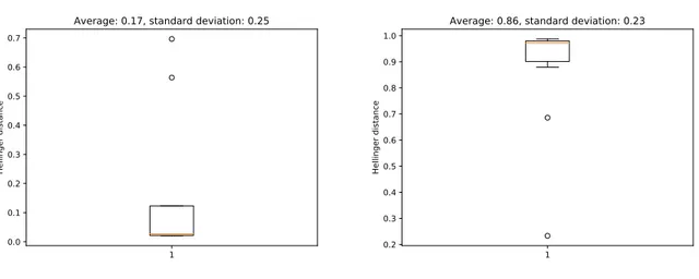
To overcome this issue, we built a scraper which samples randomly pages of wikipedia.it with replacement, using the URL https://it.wikipedia.org/wiki/Speciale:PaginaCasuale. The basic idea is that it is unlikely that a relatively small number of random pages share topics; the resulting Hellinger distance between them can be then considered noise. Fur-thermore, we must collect enough documents to have a meaningful HDP model.

For this reason, we decided to scrape 100 pages and to compute the two similarity graphs as previously done for corsi.unige.it. Since the number of Wikipedia webpages is greater than one million1, the probability of sampling the same document more than once is relatively small. Thanks to this, it was possible to have a procedure that resembles the one presented in Section 4.1.2 which filters out spurious weights given a particular p-value. This procedure was repeated 10 times with a p-value of 0.01. Results can be consulted in Figure 5.1. The averaged results were used to produce the two unweighted networks.

5.4 Data exploration

We then compared the structure of the website built through hyperlinks and the inferred networks. In this scenario, each link tag is considered an undirected and unweighted edge

(30)

1 0.0 0.1 0.2 0.3 0.4 0.5 0.6 0.7 He lli ng er d ist an ce

Average: 0.17, standard deviation: 0.25

1 0.2 0.3 0.4 0.5 0.6 0.7 0.8 0.9 1.0 He lli ng er d ist an ce

Average: 0.86, standard deviation: 0.23

Figure 5.1: Boxplot of the computed thresholds for the filtered version (left) and the unfiltered one (right).

between the URL of the webpage in which it is found and the URL of its “href” attribute. The following proprieties were analyzed:

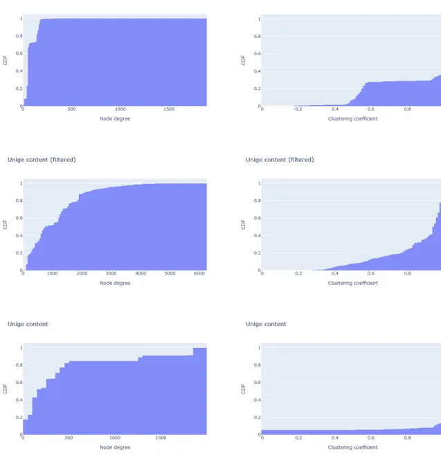
• the degree distribution • the clustering coefficient

where the clustering coefficient of a node is the number of possible triangles through that node normalized by the potential maximum number of them and the average clustering coefficient is just an average between all nodes of a graph. The histograms of the two proprieties expressed before can be seen in Figure 5.2.

Thanks to this analysis we concluded that the inferred networks and the website structure are graphs with different characteristics. In particular, the structure is sparser and less clustered than the inferred networks.

5.5 Evaluation of the results

Evaluating the quality of the result is not a trivial task.

Since we knew from Section 5.4 that the inferred networks are sparse, we focused our analysis only on the links between documents.

(31)

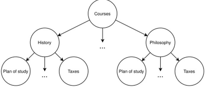
courses provided by UniGe have a particular starting page and that they share a common tree-like structure. For instance, all courses have a page called ”Orientamento” which have similar content everywhere. Figure 5.3 shows this pattern graphically.

In order to provide a score for evaluating if the inferred networks have a meaningful struc-ture, we grouped pages by their similarities (e.g. all ”Orientamento” webpages are in the same group) and we checked how many pages in the group are connected.

The results show that the unfiltered network recovers more than the 82% of the edges, while the filtered one identifies more than the 99% of them.

Courses

History Philosophy

Taxes Taxes

Plan of study Plan of study

...

... ...

Figure 5.3: Subsampling of the UniGe website structure with titles translated to English.

5.6 Scaling issues

All source code is licensed under the GNU General Public License v3.0 and it can be found at https://github.com/Davide95/msc_thesis/tree/master/code. It is written in Python 3.7 and the external libraries used are reported in the relative requirements.txt file. The source code was also analyzed with “flake8” and “pylint” to improve readability and to spot bugs.

During the writing of the source code, we encountered some scalability issues related to the size of the datasets and the computational complexity of the algorithms used. This section contains a summary of the main strategies used to overcome this problem. All experiments were tested on a PowerEdge T630 server with the following characteristics:

• Intel(R) Xeon(R) CPU E5-2630 v3 @ 2.40GHz (2 sockets) • 8x16GiB of RAM

(32)

5.6.1 NumPy

The majority of operations in our source code are applied to vectors and matrices. Modern CPUs provide SIMD (Single Instruction, Multiple Data) instructions like Intel® AVX-512 to speed up this kind of computations. In order to use them in the source code, we make use of a library called NumPy2 _{which is interoperable between different hardware and}

computing platforms.

Furthermore, it allows us to have more numerical stability when dealing with huge matrices and vectors since it takes into account the limitations related to storing real numbers using finite-precision floating-point representations (for instance, using pairwise summation in its source code at numpy/core/src/umath/loops.c.src).

The interested reader can find more advantages of using NumPy reading [vCV11].

5.6.2 Numba

When vectorization is not enough due to the computational costs of the algorithms used, we compile portions of the Python code to machine code through Numba3.

Thanks to this tool, portions of the software can: • run at native machine code speed

• run without the involvement of the Python interpreter • be parallelized using multithreading

In particular, parallelization is done releasing first the GIL (Global Interpreter Lock). The interested reader can find more details about it at https://docs.python.org/3/ glossary.html#term-global-interpreter-lock.

A basic introduction to how Numba works can be found at [LPS15].

5.6.3 Multiprocessing

We are not able to use NumPy nor Numba where the code is not numerically orientated. Furthermore, it is not possible to release the GIL in some portions of the code due to the limitations of the imported libraries. For these reasons, there are situations in which multiprocessing is used.

2

https://numpy.org/

3

(33)

In particular, we have to use multiprocessing instead of multithreading during the parsing of HTML documents explained in Section 5.2. This choice allows us to scale using every core of our machine but at the cost of increasing the memory consumption of the application. To have a trade-off between computational costs and memory issues, we decided to add two parameters that can be tweaked.

5.6.4 Optimizing memory usage

In Python, it is not possible to deallocate manually memory blocks; a GC (Garbage Col-lector) is instead responsible to remove data from memory when needed.

To help its work, we try to avoid using the Jupyter Notebook when we found high memory usage. The reason is mainly that it tends to abuse the use of the global scope for storing variables and it keeps additional references to objects. Furthermore, we split the code into different steps, each step restrained in a function. Between each step, we manually force the GC to collect unused resources.

Finally, we avoid using lists when they do not have a fixed size. The reason is that frequent append operations in a short time lead in multiple reallocations of memory which could not be deallocated in time and a memory shortage might happen. In particular, the problem is that lists in Python are not linked lists but they use exponential over-allocation every time they lack space. To make a comparison, they have the same mechanism as ArrayList in Java. For a more detailed explanation of how memory management works for lists in Python, please refer to its source code at Objects/listobject.c.

(34)

Figure 5.2: Cumulative distribution function of the node degrees (first column) and the clustering coefficients (second column). The first row is referring to the structure of the website, while the second and third row show the results respectively from the filtered similarity graph and the unfiltered one.

(35)

Chapter 6 Conclusions and future work

The main purpose of this work was to infer similarities between documents in a collection, obtaining a network in which vertices are documents and edges express similarities of the content. In particular, we worked with scraped websites showing that for our data it is possible to construct a graph of relations between thousands of webpages without scaling issues. Note that being a website is not a requirement and our pipeline can be used in the future also for datasets which are only a collection of documents.

An extension of our pipeline might be to consider the semantic tags, assigning different weights to the text inside them. An example could be to consider each title inside a “<h1>” tag twice important than text outside it, counting the words twice during the Bag-of-Words conversion.

Due to limited time, we dealt with monolingual websites, but we propose an approach to overcome this issue. The problem can be divided into two steps: an automatic identification of the language of a portion of text and the production of an algorithm to have the same Bag-of-Words representation for each concept expressed in different languages. Since we are working with web data, it is possible to retrieve the language of the content of each webpage by looking at the Content-Language entity header (see [FR14]) or the lang global attribute (see the HTML 5.1 W3C Recommendation1_{). Note that the second approach}

is preferable when “lang” is provided since it handles the situation in which at least one webpage is composed of sections with different languages. When both options are not available, a language identification model (see fastText resources2_{) could be used as a}

failover. In order to have different languages with a common Bag-of-Words representation, we could translate each document to a pre-defined language and then compute the BoW format for each document as previously done. The lack of pre-trained models covering a

1

https://www.w3.org/TR/html51/dom.html#the-lang-and-xmllang-attributes

2

(36)

wide range of languages requires to find alternative solutions to the problem of translation. we suggest to look for already trained multilingual word embeddings which are aligned in a common space (see fastText resources3) to use them to find an association between words expressing the same concept in different languages. The assumption we made in the last scenario is that words in different languages share the same meaning and for this reason different word vectors of different languages differ only on the basis of the vector space in which they are represented. The interested reader may refer to [JBMG18] for further analysis of the topic.

Preliminary results suggest that the inferred network can model relations between topics. Further analyses could be made with different datasets in order to empirically verify what we observed with our data. In particular, we propose Cora4 since it provides a network of connections between documents that can be used as a ground truth.

3

https://fasttext.cc/docs/en/english-vectors.html

4

(37)

Appendix A

Neural Networks

The goal of this appendix is to give a simple albeit incomplete introduction of Neural Networks for those readers who do not have a solid background on them but still they are interested in Chapter 2.

A.1 Gradient descent

Given a minimization problem 𝑚𝑖𝑛𝑤𝑓 (𝑤), 𝑤 ∈ R𝐷, it is possible to find a local minimum

through gradient descent.

First, we compute the gradient ∇𝑓 (𝑤) and we decide a point 𝑤0 in which the algorithm

has to start. If the problem is not convex, choosing a different 𝑤0 could lead to a different

solution. Since gradients point in the direction of fastest increase, we take small steps towards the opposite direction in order to reach a minimum.

The step size is controlled by a hyperparameter 𝜆: values too small for a particular problem increase the time needed to obtain a good solution and it can lead to a local minimum; values too big prevent convergence.

The final equation is:

𝑤𝑖+1= 𝑤𝑖− 𝜆∇𝑓 (𝑤𝑖)

Each step is run iteratively until a stopping criterion is met. If the algorithm is stopped after 𝐼 iterations, the solution for the minimization problem is 𝑤𝐼. Common sense stopping

criterions could be:

• stop after a prefixed number of iterations

(38)

• stop when 𝑓(𝑤𝑖) − 𝑓 (𝑤𝑖+1) < 𝜖, with 𝜖 > 0 small

Note that the parameter 𝜆 could be different at each iteration:

𝑤𝑖+1= 𝑤𝑖− 𝜆𝑖+1∇𝑓 (𝑤𝑖)

For instance, we could have 𝜆𝑖 = 𝜆_𝑖 in order to take smaller and smaller steps until

conver-gence.

A.1.1 Gradient descent in action

Suppose to have a dataset 𝑋 ∈ R𝑁 ×𝐷_{, 𝑦 ∈ R}𝑁_.

What we want to do is linear regression, whose model is obtained resolving:

min 𝑤∈R𝐷 1 2𝑁 ∑︁ 𝑖∈[1,𝑁 ] (𝑤𝑇𝑥𝑖− 𝑦𝑖)2 The derivative _2𝑁1 ∑︀ 𝑖(𝑤 𝑇_𝑥 𝑖− 𝑦𝑖)2𝑑𝑤 is: 1 2𝑁 ∑︁ 𝑖∈[1,𝑁 ] 2𝑥𝑖(𝑤𝑇𝑥𝑖− 𝑦𝑖) = ∑︀ 𝑖∈[1,𝑁 ]𝑥𝑖(𝑤 𝑇_𝑥 𝑖− 𝑦𝑖) 𝑁 Therefore: 𝑤𝑛+1 = 𝑤𝑛− 𝜆 𝑁 ∑︁ 𝑖∈[1,𝑁 ] 𝑥𝑖(𝑤𝑇𝑖 𝑥𝑖− 𝑦𝑖)

A.2 Mini-batch gradient descent

There are situations in which using gradient descent is not computationally feasible. For instance, imagine that the problem explained in Section A.1.1 have a number of points so huge that a solution cannot be obtained in feasible times.

Mini-batch gradient descent is an extension of gradient descent which assumes that samples of |𝑀 | elements of the dataset are a noisy representative of the entire data. At each step, 𝑀 will be re-sampled from 𝑋.

In that case, the minimization presented in Section A.1.1 can be rewritten as:

min 𝑤∈R𝐷 1 2|𝑀 | ∑︁ 𝑥𝑖∈𝑀 (𝑤𝑇𝑥𝑖− 𝑦𝑖)2

(39)

A.3 Linear Neural Networks

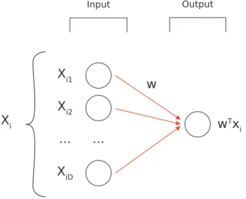
The linear regression exposed in Section A.1.1 can be viewed as a Neural Network which has 𝐷 inputs as a first layer and a single neuron as output connected to all previous ones. The graphical representation of it can be seen in Figure A.1.

The vector 𝑤 is simply the set of all weights. Starting from the equation presented in Section A.1.1: 𝑤𝑛+1 = 𝑤𝑛− 𝜆 𝑁 ∑︁ 𝑖∈[1,𝑁 ] 𝑥𝑖(𝑤𝑇𝑥𝑖− 𝑦𝑖)

each weight 𝑤𝑖 can be parallelly updated:

𝑤(𝑛+1)𝑗 = 𝑤𝑛𝑗 − 𝜆 𝑁 ∑︁ 𝑖∈[1,𝑁 ] 𝑥𝑖𝑗(𝑤𝑇𝑥𝑖− 𝑦𝑖)

In this example, the cost function is the square loss, but there is not any particular re-quirement when dealing with Neural Networks.

Output Input X_i1 X_i2 XiD ... ... w T_x i Xi w

Figure A.1: A graphical representation of a linear Neural Network.

A.4 Activation functions

In each node, a non-linear function could be applied at the data before moving the output to the next layer. For the sake of simplicity, we are going to present a model similar to the

(40)

previous one, with the difference that a tanh(·) function is applied to the output node: min 𝑤∈R𝐷 1 2𝑁 ∑︁ 𝑖∈[1,𝑁 ] [tanh(𝑤𝑇𝑥𝑖) − 𝑦𝑖]2

To resolve it with gradient descent, we have to apply the chain rule. Since tanh(𝑧)𝑑𝑧 = 1 − 𝑡𝑎𝑛ℎ2_(𝑧): 1 2𝑁 ∑︁ 𝑖∈[1,𝑁 ] [tanh(𝑤𝑇𝑥𝑖) − 𝑦𝑖]2𝑑𝑤 = 1 2𝑁 · ∑︁ 𝑖∈[1,𝑁 ] 2[tanh(𝑤𝑇𝑥𝑖) − 𝑦𝑖] · [1 − 𝑡𝑎𝑛ℎ2(𝑤𝑇𝑥𝑖)] · 𝑥𝑖 𝑤𝑛+1 = 𝑤𝑛− 𝜆 𝑁 ∑︁ 𝑖∈[1,𝑁 ] [tanh(𝑤𝑇𝑥𝑖) − 𝑦𝑖][1 − 𝑡𝑎𝑛ℎ2(𝑤𝑇𝑥𝑖)]𝑥𝑖

Other activation functions can be used instead of tanh(·). The one used in the models presented in Chapter 2 is the softmax 𝜎(𝑧), 𝑧 ∈ R𝑉:

𝜎(𝑧, 𝑗) = 𝑒 𝑧𝑖 ∑︀ 𝑗𝑒𝑧𝑗 𝜎(𝑧) = ⎡ ⎢ ⎢ ⎣ 𝜎(𝑧, 1) 𝜎(𝑧, 2) ... 𝜎(𝑧, 𝑉 ) ⎤ ⎥ ⎥ ⎦

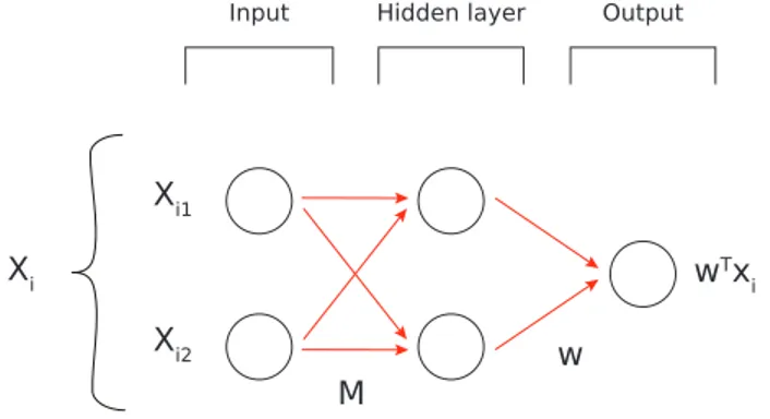
A.5 Multilayer Neural Networks

Adding intermediate layers (usually called hidden layers in the literature) to a linear Neural Network is useless since the product of linear components is again linear. As an example, construct a model with the following characteristics:

• 𝑋 ∈ R𝑁 ×2_{: 2 nodes as input}

• 𝑦 ∈ R𝑁_{: 1 node as output}

• 2 nodes in the hidden layer, fully connected to the two other layers

Its graphical representation can be seen in Figure A.2 and the relative minimization func-tion is: min 𝑀,𝑤 1 2𝑁 ∑︁ 𝑖∈[1,𝑁 ] [𝑤𝑇(𝑥𝑖𝑀 ) − 𝑦𝑖]2 with 𝑀 ∈ R2×2, 𝑤 ∈ R2

(41)

which is again linear regression but more computationally expensive.

On the opposite, stacking more layers while using a non-linear activation function leads to an enriched hypothesis space. Learning weights in a Deep Neural Network (a Neural Network with multiple hidden layers) requires using the backpropagation algorithm.

Output Input X_i1 X_i2 wT_x i Xi w Hidden layer M

Figure A.2: A graphical representation of a Neural Network with an hidden layer.

A.5.1 Chain rule

The chain rule states that given ^𝑦 = 𝑓 (𝑔(𝑥)) its derivative is:

𝑑^𝑦 𝑑𝑥 = 𝑓 (𝑔) 𝑑𝑔 · 𝑔(𝑥) 𝑑𝑥

That formula can be seen as a Neural Network with one node as input, one as output and one in the hidden layer. Its graphical representation can be viewed in Figure A.3.

Output Input

x

Hidden layer

g(x)

f(g)

(42)

A.6 Backpropagation

To better understand backpropagation, imagine having a fully connected Neural Network with:

• 𝐷 nodes as input

• 𝐽 nodes in the hidden layer with tan as activation function • 1 node as output with tan as activation function

This network has weights 𝑀 ∈ R𝐷×𝐽 _{between the first and the second layer, and weights}

𝑤 ∈ R𝐽 _{connecting the second layer to the third.}

The minimization function is

min 𝑀,𝑤 1 2 ∑︁ 𝑖∈[1,𝑁 ] 𝐸(𝑋, 𝑦)𝑖 = min 𝑀,𝑤 1 2 ∑︁ 𝑖∈[1,𝑁 ] {tanh[𝑤𝑇 _tanh(𝑋 𝑖𝑀 )] − 𝑦𝑖}2

The final goal is to obtain:

• 𝑑𝐸𝑖

𝑑𝑤 •

𝑑𝐸𝑖

𝑑𝑀𝑑𝑗

In order to make the notation as light as possible, the function tanh(·) is intended to be applied element-wise. Moreover, the intermediate result tanh(𝑀 𝑋𝑖) is denoted as ℎ𝑖 and

the symbol ∘ represents the element-wise product between two vectors.

To compute the partial derivatives, we can start from the output layer and then use the intermediate calculations to compute the partial derivatives of the previous layers. In particular: 𝑑𝐸𝑖 𝑑𝑦𝑖 = 1 2 · 2{tanh[𝑤 𝑇 tanh(𝑀 𝑋𝑖)] − 𝑦𝑖} = tanh(𝑤𝑇ℎ𝑖) − 𝑦𝑖 𝑑𝐸𝑖 𝑑𝑤 = 𝑑𝐸𝑖 𝑑𝑦𝑖 𝑑𝑦𝑖 𝑑𝑤 = 𝑑𝐸𝑖 𝑑𝑦𝑖

{1 − tanh2[𝑤𝑇 tanh(𝑀 𝑋𝑖)]} tanh(𝑋𝑖𝑀 )

𝑑𝐸𝑖 𝑑ℎ𝑖 = 𝑑𝐸𝑖 𝑑𝑦𝑖 𝑑𝑦𝑖 𝑑ℎ𝑖 = 𝑑𝐸𝑖 𝑑𝑦𝑖 {1 − tanh2_[𝑤𝑇 _{tanh(𝑀 𝑋} 𝑖)]}𝑤 𝑑𝐸𝑖 𝑑𝑀𝑑𝑗 = [𝑑𝐸𝑖 𝑑ℎ𝑖 ∘ {1 − tanh2_(𝑋 𝑖𝑀 )]}𝑗𝑋𝑖𝑑

The power of this technique is that it is possible to re-use values calculated for a particular partial derivative to lower the computational cost of computing the others.

(43)

A.7 References

Details are omitted and the topic is discussed only in summary fashion, although the reference paper is provided for the interested reader: [Ron14].

(44)

Appendix B

Probability distributions

Over all probability distributions used in this document, some of them are not usually part of the canonical background of a computer scientist. We decided to present them in this appendix in order to have an overview for who has never seen them before.

B.1 Beta distribution

The Beta distribution is a family of continuous probability distributions. It is defined in the range [0, 1] and it has two parameters 𝛼, 𝛽 > 0.

Since 𝛼 and 𝛽 are concentration parameters, they induce more and more sparsity as they approach the value of zero. If 𝛼 = 𝛽 = 1, the probability density function is uniform over [0, 1]. As their values grow, the distribution tightens over its expectation. All these observations can be seen empirically in Figure B.1.

Due to its characteristics, it is suited to model probabilistic outcomes (for example, to describe how confident we are about the fact that a coin is loaded or not).

B.1.1 Probability density function

Given a random variable 𝑋 ∼ Beta(𝛼, 𝛽), the probability density function is defined as:

𝑓𝑋(𝑥) =

1 𝐵(𝛼, 𝛽)𝑥

𝛼−1

(45)

0.0 0.2 0.4 0.6 0.8 1.0 x 0.0 0.5 1.0 1.5 2.0 2.5 3.0 3.5 fX (x ) α=1, β=0.5 α=0.5, β=1 α=1, β=1 α=1.5, β=2

Figure B.1: Example of the probability density function of a Beta distribution varying its parameters.

𝐵(𝛼, 𝛽) is the Beta function and it acts as a normalization constant to ensure that:

∫︁ 1

0

𝑓𝑋(𝑥)𝑑𝑥 = 1

B.2 Dirichlet distribution

The Dirichlet distribution is a family of multivariate distributions. It is parametrized by 𝐾 parameters, where 𝐾 is the number of random variables for which it is described. It can be seen as a generalization of the Beta distribution: a Dirichlet distribution of 2 parameters Dir (𝛼1 = 𝑎, 𝛼2 = 𝑏) is a Beta distribution Beta(𝛼 = 𝑎, 𝛽 = 𝑏). All

considera-tions and constraints about the parameters of the Beta distribution presented previously (Section B.1) still holds for the Dirichlet distribution.

B.2.1 Probability density function

Given a multivariate random variable 𝑋 ∼ Dir (𝛼1, 𝛼2, . . . , 𝛼𝐾), the probability density

(46)

𝑓𝑋(𝑥1, 𝑥2, . . . , 𝑥𝐾; 𝛼1, 𝛼2, . . . , 𝛼𝐾) = 1 𝐵(𝛼1, 𝛼2, . . . , 𝛼𝐾) 𝐾 ∏︁ 𝑖=1 𝑥𝛼𝑖−1 𝑖

𝐵(𝛼1, 𝛼2, . . . , 𝛼𝐾) is the multivariate generalization of the Beta function presented in

Sec-tion B.1.

Setting Dir (𝛼) := Dir (𝛼1, 𝛼2, . . . , 𝛼𝑛), a simplified notation of the probability density

function is used: 𝑓𝑥(𝑥1, 𝑥2, . . . , 𝑥𝐾; 𝛼) = 1 𝐵(𝛼) 𝐾 ∏︁ 𝑖=1 𝑥𝛼−1_𝑖

The support is constrained by: • 𝑥𝑖 ∈ (0, 1), 1 ≤ 𝑖 ≤ 𝐾

• ∑︀𝐾

𝑖=1𝑥𝑖 = 1

B.2.2 Graphical intuition

The support of a Dirichlet distribution with 𝐾 parameters lies in a 𝐾 − 1 simplex. If 𝐾 = 3, the simplex is a triangle and can be represented graphically (see Figure B.2). All values of the probability density function 𝑓𝑋(𝑥1, 𝑥2, 𝑥3) : ℜ3− > ℜ are associated with

a specific color given their intensity. Bigger values in the probability density function are represented with lighter colors and vice versa.

Vertices of the simplex represent the situations in which 𝑥 =[︀1 0 0]︀, 𝑥 = [︀0 1 0]︀ or 𝑥 =[︀0 0 1]︀. If 𝑥 = [︀1₃ 1₃ 1₃]︀, we are at the center of the simplex. Given an area of the triangle lighter than others, the probability of obtaining a vector in that interval during sampling is higher and vice versa.

Suppose we are in a supermarket and we are interested in the kind of purchases con-sumers make. We define three categories: “food”, “technology” and “stationery”. A strong preference over one category is represented modelling the probability density func-tion with higher values towards one of the vertices. Sampling from a Dirichlet distribufunc-tion as the one represented in the left simplex in Figure B.2 will tend to give us users who do not have a strong preference over one category. The opposite situation (for example, 𝛼1 = 0.1, 𝛼2 = 0.1, 𝛼3 = 0.1) will otherwise give us customers who strongly prefer one of

the categories (for example. 𝑥 = [︀0.8 0.15 0.05]︀) while users without propensities will be much rare. Finally, if the probability density function is uniform over all the support (right simplex in Figure B.2) there is no tendency of choosing a particular combination of categories over others.

(47)

Figure B.2: Example of the probability density function over a simplex of a Dirichlet distribution varying its three parameters 𝛼 = (𝛼1, 𝛼2, 𝛼3). The lighter the color, the higher

the probability density function.

B.3 Categorial distribution

The categorical distribution is a generalized Bernoulli distribution in the case of categorical random variables.

In the literature about Topic Modeling, it is wrongly used with the name of Multinomial distribution. To keep the same notation as the papers in the bibliography, we will say that 𝑋 ∼ Mult (𝑝) means that X is distributed as Categorical. Note that a Categorical distribution Mult (𝑝) is a special case of a Multinomial distribution Mult (𝑛, 𝑝) in which 𝑛 = 1.

Each 𝑝𝑖 of the parameter 𝑝 = (𝑝1, 𝑝2, . . . , 𝑝𝐾) represents the probability of observing 𝑖 by

sampling from the distribution.

B.3.1 Probability mass function

Given a random variable 𝑋 ∈ Mult (𝑝), the probability mass function is defined as:

(48)

B.4 References

The interested reader may refer to [Gup11], [BNJ03] and [Seb11] to use them as refer-ences.

(49)

Appendix C

Probability distributions closeness

Some methods were developed to assess closeness between different probability distribu-tions (see Figure C.1).

In this appendix, we cover the ones which are used in the thesis.

−3 −2 −1 0 1 2 3 x 0.0 0.1 0.2 0.3 0.4 0.5 0.6 0.7 0.8 PDF (x ) −3 −2 −1 0 1 2 3 x 0.00 0.25 0.50 0.75 1.00 1.25 1.50 1.75 2.00 PDF (x )

Figure C.1: On the left plot the probability density function of two close distributions, the opposite on the right plot.

(50)

C.1 Kullback–Leibler divergence

Given two probability distributions 𝑝(𝑥) and 𝑞(𝑥), we define the KL divergence as:

KL(𝑝‖𝑞) = ∫︁ 𝑥 𝑝(𝑥) log₂ 𝑝(𝑥) 𝑞(𝑥) = E𝑝[log2 𝑝(𝑥) 𝑞(𝑥)]

If the two distributions are discrete, it can be rewritten as:

KL(𝑝‖𝑞) =∑︁

𝑖

𝑝(𝑖) log₂ 𝑝(𝑖) 𝑞(𝑖)

Suppose we have two Categorical distributions 𝑐1and 𝑐2with parameters 𝑝𝑐1 = (0.1, 0.2, 0.7)

and 𝑝𝑐2 = (0.3, 0.5, 0.2), respectively.

Given the formula presented above, we can compute the KL divergence: • KL(𝑐1‖𝑐2) = 0.1 log2 0.10.3 + 0.2 log2 0.20.5 + 0.7 log2 0.70.2 ≈ 0.85

• KL(𝑐2‖𝑐1) = 0.3 log2 0.3 0.1 + 0.5 log2 0.5 0.2 + 0.2 log2 0.2 0.7 ≈ 0.77

C.1.1 Proprieties

From the previous example, it can be seen that the KL divergence is not symmetric: KL(𝑝‖𝑞) ̸= KL(𝑞‖𝑝).

Also, note that KL(𝑝‖𝑝) = ∫︀

𝑥𝑝(𝑥) log2 𝑝(𝑥) 𝑝(𝑥) = ∫︀ 𝑥𝑝(𝑥) log2(1) = ∫︀ 𝑥𝑝(𝑥) · 0 = 0 and KL(𝑝‖𝑞) ≥ 0.

C.2 Hellinger distance

The Hellinger distance has some advantages over the Kullback–Leibler divergence: • it is symmetric: HD(𝑝, 𝑞) = HD(𝑞, 𝑝)

• it has an upper bound: 0 ≤ HD(𝑝, 𝑞) ≤ 1

Given two discrete probability distributions 𝑝 and 𝑞, the Hellinger distance is defined as:

HD (𝑝, 𝑞) = HD (𝑞, 𝑝) = √1 2 √︃ ∑︁ 𝑖 (√︀𝑝(𝑖) −√︀𝑞(𝑖))2

Note that in the literature the Hellinger distance is defined in different ways (e.g. with or without √1

(51)

C.3 References

The interested reader may refer to [Joy11], [Lin91] and [Hel09] for further analysis of the topic.

Apprendimento automatico delle relazioni fra documenti dal web

Learning relational models

from networked data on the web

Davide Riva

Master Thesis

MSc Computer Science

Learning relational models

from networked data on the web

Davide Riva

Advisors: Annalisa Barla, Davide Garbarino

Examiner: Nicoletta Noceti

Abstract

Contents

Chapter 1

Introduction and motivation

Chapter 2

Word Embedding

2.1

One Hot Encoding

2.2

Word2vec

2.2.1

Continuous Bag-of-Words Model (CBOW)

2.2.2

Continuous Skip-gram Model (Skip-gram)

2.2.3

Interpretation of the results

2.3

Global Vectors (GloVe)

2.4

Measuring distances between terms

Chapter 3

Topic Modeling

3.1

Latent Semantic Analysis (LSA)

X

≃

U Σ V

3.2

Latent Dirichlet Allocation (LDA)

3.2.1

Generative process

3.2.2

Model inference

3.2.3

Sparsity considerations

3.3

Online LDA

3.4

Hierarchical Dirichlet process (HDP)

3.4.1

Dirichlet process (DP)

3.4.2

HDP nesting DPs

Chapter 4

Network inference

4.1

ARACNE

4.1.1

Computation of Mutual Information (MI) between genes

4.1.2

Identification of a meaningful threshold

4.1.3

Data Processing Inequality (DPI)

Chapter 5

Experiments

5.1

Crawling

5.2

Similarity graph

5.3

Weight binarization of the network

5.4

Data exploration

5.5

Evaluation of the results

5.6

Scaling issues

5.6.1

NumPy