A Feature Tracking Velocimetry technique applied to inclined negatively
buoyant jets
Simone Ferrari
1,*, Maria Grazia Badas
1, Luigi Antonio Besalduch
1, Giorgio
Querzoli
11: DICAAR, Dipartimento di Ingegneria Civile, Ambientale e Architettura, University of Cagliari, Cagliari, Italy * correspondent author: [email protected]
Abstract We have applied a Feature Tracking Velocimetry (FTV) technique to measure displacements of particles on
inclined negatively buoyant jets (INBJs), issuing from a circular sharp-edged orifice, in order to investigate, among the others, the symmetry properties of the velocity field on this phenomenon. Feature Tracking Velocimetry is less sensitive to the appearance and disappearance of particles and to high velocity gradients than classical Particle Image Velocimetry (PIV). The basic idea of Feature Tracking Velocimetry is to compare windows only where the motion detection may be successful, that is where there are high luminosity gradients. The Feature Tracking Velocimetry algorithm presented here is suitable in presence of different seeding densities, where other techniques produce significant errors, due to the non-homogeneous seeding at the boundary of a flow. The Feature Tracking Velocimetry algorithm has been tested on laboratory experiments regarding simple jets (SJs) and inclined negatively buoyant jets released from a sharp-edged orifice. We present here velocity statistics, from the first to the fourth order, to study, among the others, the differences between simple jets and inclined negatively buoyant jets, and to investigate how the increase in buoyancy affects the inclined negatively buoyant jet behavior. We remark that, to the best of authors’ knowledge, this is the first attempt to investigate velocity statistics of an order higher than the second on Inclined Negatively Buoyant Jets. Among the others quantities, the mean streamwise velocity decay and the integral Turbulent Kinetic Energy have been measured and analyzed, both along the jet axis and in the upper and lower region of the simple jets and inclined negatively buoyant jets, as well as the streamwise and spanwise velocity skewness and kurtosis evolution along the axis. Results show the role of buoyancy in modifying the inclined negatively buoyant jet features; moreover, it is highlighted that the asymmetry of inclined negatively buoyant jets cannot be considered only a far field feature of this phenomenon, as it arises very close to the release point.
1. Introduction
When a fluid is released upwards into a lighter receiving fluid or downwards into a heavier one, the physical phenomenon that develops is called negatively buoyant jet. As far as the release is vertical, this is a deeply investigated symmetric phenomenon but, as soon as the release has a different inclination, the misalignment between the initial momentum and the buoyancy determines a much more complex phenomenon.
The previous investigations on inclined negatively buoyant jets (INBJs) available in scientific literature (e.g. Roberts et al., 1997; List et al., 1979) have highlighted a symmetric simple-jet-like behavior, near to the origin, followed by an asymmetric one, with a larger widening of the lower region compared to the upper one. Conversely, from some previous investigations carried out in our laboratories (Besalduch et al., 2013 and 2014), with more practical targets, the second order statics of the velocity field has shown that this lack in symmetry arises very close to the origin. In order to deeply investigate this apparent contradiction, we have performed a new experimental campaign focusing on the behavior of inclined negatively buoyant jets. In this work, the near field of an INBJ is defined as the region between the origin and the point of maximum height, as in this point the interaction between the upward branch and the downward one deeply affects the physics of the phenomenon.
There are many practical applications: of INBJs: sea discharges of effluents from wastewater treatment plants (Koh and Brooks, 1975) or form desalination plants (Lai and Lee, 2012), exit snow from snow ploughs (Lindberg and Petersen, 1991), sand and slurry jets as dredging and island building operations and pulverized coal combustion (Hall et al 2010). One of the most important applications are certainly sea discharge of brine from desalination plants through submerged outfalls (e.g. Ferrari et al, 2010; Cipollina et al., 2005), due to large diffusion of this kind of plants, made to cope the increase of water request in particular in arid region.
In this work INBJs were emitted from a sharp edged orifice; this kind of release, although being a common operative configuration in discharge since it has been thoroughly investigated in literature with respect to the ones released at the end of a long pipe or with a smooth contraction, moreover the former configuration determines more complex phenomena than the latter, for example due to the inward radial component of the velocity, that is apparent in the well known vena contracta, or the unsteadiness due to the upstream separation, Mi et al., 2001 and 2007.
To perform the velocity measurements, a Feature Tracking Velocimetry (FTV) technique has been developed and employed, with the target to overcome some issues of classical Particle Image Velocimetry (PIV) algorithms. As a matter of fact, as PIV algorithms obtain velocity fields comparing windows of successive frames on a regular grid in all the image and maximizing the correlation of the light intensity function to obtain their displacement, they are typically very sensitive to the appearance and disappearance of particles, to high velocity gradients and do not work properly where there are different seeding densities in the investigation field (e.g., between a jet and the external fluid, where the seeding cannot be homogeneous). Differently, FTV is based on the idea of comparing windows only where the motion detection may be successful, that is where there are high luminosity gradients.
2. Relevant non-dimensional parameters
In an INBJ the flow is driven from two sources, one of momentum and one of buoyancy: the first region of the jet is driven mostly by the momentum (so it behaves similarly to a simple jet released with the same angle); far from the outlet, there is a second region where the buoyancy acts to bend the axis down (so the jet behaves similarly to a plume) (List, 1979). The most relevant non-dimensional parameter for the classification of buoyant jets is the densimetric Froude number, Fr:
D g U Fr REC DISC REC 0 ρ ρ ρ − = (1)
where U0 is the mean initial jet velocity, g the gravitational acceleration, ρDISC the discharged fluid density,
ρREC the receiving fluid density and D the outlet diameter. Fr, being the ratio between inertial and buoyancy
forces, has low values for heavy jets and high values as buoyancy decreases, up to an infinite value for simple jets.
The other relevant non-dimensional parameters in INBJs are the Reynolds number, Re = U0D / υ (υ is the
kinematic viscosity of the discharged fluid), and the angle to the horizontal, θ. This last parameter controls the misalignment between the flux of buoyancy and the initial flux of momentum: as a consequence, an INBJ is axisymmetric only as far as θ is 90°.
3. Laboratory set-up
The laboratory section was set-up in order to reproduce a standard configuration of sea discharge, i.e. a portion of pipe, laid down on the sea floor, which discharges the effluent from the orifices along its wall (Wright et al.,1982; Avanzini et al., 2006). The experimental set-up simulates a portion of a pipe laid down on the sea bottom, which discharges the effluent from orifices along the pipe wall, a typical configuration of submarine outfalls. The model consists in a flume with glass walls, filled with water, to simulate a stagnant receiving body. The discharge comes through a pipe, which is connected to a constant head tank, by means of a cylindrical vessel diameter, with a sharp-edge orifice. The released fluid is a solution of water, pollen particles (for the visualization of the jet), to retrieve velocity fields, and sodium sulphate, in case of INBJs, to increase the density. A pumped diode laser illuminates the mean vertical plane of the diffuser, where images are recorded by means of a high speed camera, 400 fps at full spatial resolution (1728×2240). The experiments were performed with a constant flow rate (and high enough to have Re = 1500, larger than its critical value for the apparatus), Fr = 14 ÷ 37.2, θ = 65°. A simple jet (Re = 1500) was experimentally
simulated as well for comparison.
The adopted set-up is described in more details in Besalduch et al., 2013.
4. The Feature Tracking Velocimetry (FTV) technique
As previously stated, velocity fields were obtained, from each couple of images, using a novel algorithm, namely Feature Tracking Velocimetry (FTV), which is less sensitive to the appearance and disappearance of particles, and to high velocity gradients than classical Particle Image Velocimetry (PIV). PIV algorithms obtain velocity fields comparing windows of successive frames on a regular grid covering all the images and minimizing the dissimilarity between the light intensity function to obtain their displacement. The idea of FTV is to compare windows only where the motion detection may be successful, that is where there are high luminosity gradients. The FTV algorithm is suitable in presence of different seeding density, for example between the jet and the external fluid, where other techniques produce significant errors, due to the non-homogeneous seeding at the boundary.
The procedure of analysis consists of the following steps:
• identifying the features to track using the Harris corner detection (a corner is a region with high luminosity gradients along the x and y direction) (Harris & Stephens, 1988);
• sorting the features according to their cornerness (i.e. the value of the Harris formula);
• selecting the first N features and computation of velocity comparing a window centered with the ith feature (Wt) with windows (Wt+1) with a range of displacements, (di, dj) in the next frame;
• measuring, for each displacement, the dissimilarity, d(di, dj), between Wt and Wt+1(di, dj) by means
of the Lorentzian estimator; and hence obtaining the velocity as the displacement minimizing the dissimilarity;
Samples are later validated with the following algorithm, based on Gaussian filtering of first neighbors (defined by the Delaunay triangulations) and on simulated annealing, with the following steps:
• for each set of sparse velocity samples the Delaunay triangulation is computed;
• for each sample, an interpolation of the value of the first neighbors (following the Delaunay triangulation) is computed using a Gaussian weighted average;
• the difference between the velocity sample and the interpolated value is computed for every sample; • if the measured sample giving the larger difference exceeds a given threshold (a parameter of the
method), this measured sample is substituted with the interpolation of its neighbors and the steps 2-4 are repeated until all differences are below the threshold.
Under the hypothesis of ergodicity, the statistics of velocity fields are obtained by time averaging.
This technique is suitable for measurements from a wide range of seeding density: from the high level typical of PIV down to the low seeding which is characteristic of PTV (Particle Tracking Velocimetry). Moreover, it is suited to the analysis of images with intermediate seeding density or non-homogeneous seeding.
A comparison among FTV and some other classical PIV techniques have been performed on the data from present experiments: the comparison shows a good performance of FTV, which provides better results than regular grid based methods especially at shear layer at the border of the jets, leading to sharper fields and more reliable estimation of second order statistics.
5. Results
In this chapter, we will show before the first order statistics obtained from velocity fields and the physical conclusions we can draw from them, to then focus on the second order ones and on the deeper information these last are able to produce and, eventually, illustrate the streamwise and spanwise velocity skewness (third order) and kurtosis (fourth order) evolution along the axis. We remark that, to the best of authors’ knowledge, this is the first attempt to investigate velocity statistics of an order higher than the second on Inclined Negatively Buoyant Jets.
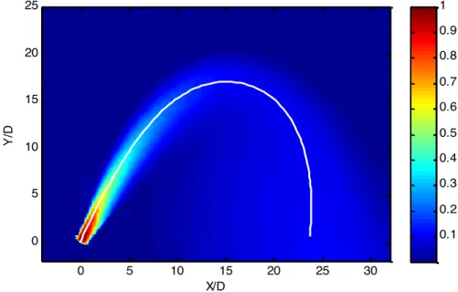
In Figure 1, the mean velocity field U, normalized by the maximum velocity at the outlet Umax, for an
Inclined Negatively Buoyant Jet with Fr = 8, Re = 1000, and θ = 65° is shown; this allows to highlight the general features of INBJs. The jet axis is defined as the locus of maximum intensity velocity on sections orthogonal to the jet; on Figure 1 it is superimposed to the velocity field as a white line. As stated before, an INBJ is driven by two forces acting in different directions, namely momentum and buoyancy. As shown in Figure 1, INBJs cover a very short initial distance, where they seem to be driven essentially by the initial momentum and maintain a width similar to the diameter of the orifice D while, after this distance, the onset of the Kelvin-Helmholtz billows causes the widening of INBJs. As the distance from the orifice increases, the buoyancy becomes more and more relevant, finally bending the jet downwards. After this point, where the INBJs reach their maximum height, they behave, in their descending branch, similarly to a plume. Figure 1 shows how this descending branch experiences a sudden widening at Y/D ≈ 10, due to the interaction between the upward branch and the downward one. As a matter of fact, the mean velocities in the upward branch tend to balance with the ones in the descending branch, preventing a larger widening of this last one.
Figure 1. Map of the non-dimensional mean velocity U/Umax (Umax is the maximum velocity at the outlet) for an INBJ
with Re = 1000, Fr = 8, q = 65°; the white line is the jet axis (defined as the locus of maximum intensity velocity)
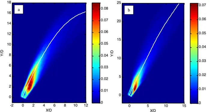
As here we focus on the symmetry properties of the near field of INBJs (defined as the region ranging from the jet's origin to the point of maximum height, where the interaction between the upward and downward branches strongly complicates the physics of the phenomenon), on Figure 2 we show the mean velocity field U, normalized by Umax, in the near field of two INBJs (with Re = 1000, θ = 65° and two different Fr: Fr = 8
and 15; Figure 2a and 2b respectively). The two panels of the Figure 2 show a compact jet core near the jet origin, while at few diameters from the orifice the different stratifications in the upper and lower region of the jet (stable the former and unstable the latter) cause a clear asymmetric development of the INBJs: they widen more in the lower region, where the evolution of the Kelvin-Helmholtz billows is favored by the unstable stratification. From another point of view, it is possible to see how the velocity core (inner region with the highest velocities) and, consequently, the INBJ axis tend to be closer to the upper boundary of the jet than to the lower one. This can be explained with the detachment of descending plumes that tends to erode the velocity core more in the lower region than in the upper one. This lack of symmetry is more evident for the heavier INBJ (with Fr = 8, Figure 2b), whose axis bends at a shorter non-dimensional distance s/D from the origin, with respect to the lighter one (with Fr = 15, Figure 2a). s/D is the abscissa measured streamwise along the axis from the origin.
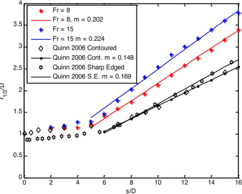
In Figure 3, the widening of two INBJs with Re = 1000, θ = 65° and two different Fr (8 in red and 15 in blue) is measured along the axis and plotted, versus s/D, together with the simple jet data (Fr = ∞) by Quinn, 2006, issuing from a sharp edged orifice (black stars) and from a contoured nozzle (black rhombi). The
X/D Y/ D 0 5 10 15 20 25 30 0 5 10 15 20 25 0.1 0.2 0.3 0.4 0.5 0.6 0.7 0.8 0.9 1
observed behaviour highlights the role of the densimetric Froude number Fr in the widening of INBJs, which is defined, for each s/D, as the orthogonal to the axis non-dimensional distance r1/2/D between the two points,
in the upper and lower region, where the velocity assumes a value which is half of the axial velocity.
Figure 2. Map of the non-dimensional mean velocity U/Umax in the near-field of an INBJ with Re = 1000, q = 65°,
Fr = 8 (a) and 15 (b); the white line is the jet axis.
Figure 3. Widening of INBJs with Re = 1000, q = 65°, Fr = 8 (red) and 15 (blue) and of two simple jets (Quinn, 2006; sharp-edged orifice: black stars; contoured orifice: black rhombi); s/D is the abscissa measured streamwise along the axis from the origin; the straight lines are the best fit ones in a least mean square sense; the coefficient m in the legend
is the inclination of the straight lines.
X/D Y/ D -2 0 2 4 6 8 10 12 0 2 4 6 8 10 12 14 16 18 0.1 0.2 0.3 0.4 0.5 0.6 0.7 0.8 0.9 1 X/D Y/ D 0 5 10 15 0 5 10 15 20 25 0.1 0.2 0.3 0.4 0.5 0.6 0.7 0.8 0.9 1 0 2 4 6 8 10 12 14 16 0 0.5 1 1.5 2 2.5 3 3.5 4 s/D r 1/2 /D Fr = 8 Fr = 8, m = 0.202 Fr = 15 Fr = 15 m = 0.224 Quinn 2006 Contoured Quinn 2006 Cont. m = 0.148 Quinn 2006 Sharp Edged Quinn 2006 S.E. m = 0.169
Figure 3 highlights the role of the buoyancy, as the Reynolds number is the same for the two INBJs: both the INBJs widens more than simple jets and that their widening rate after the initial stage (from s/D ≈ 6 onwards) is higher than the simple jets ones. In order to measure this widening rate, which is relevant as it is proportional to the entrainment and so to the dilution, the data for each case, starting from the point where the widening rate becomes substantially constant, have been fitted, in a least mean square sense, with a straight line. The widening rate, measured by the inclination m of the straight line, of the INBJs is always larger than the one of the simple jets. Moreover, the widening rate of the lightest INBJ (m = 0.224) is higher than the one of the heavier INBJ (m = 0.202), highlighting the role of Fr in the widening of INBJs: as Fr decreases (buoyancy increases), the buoyancy tends to prevail on the momentum and INBJs tend to remain confined in a smaller space, consequently experiencing a lower widening.
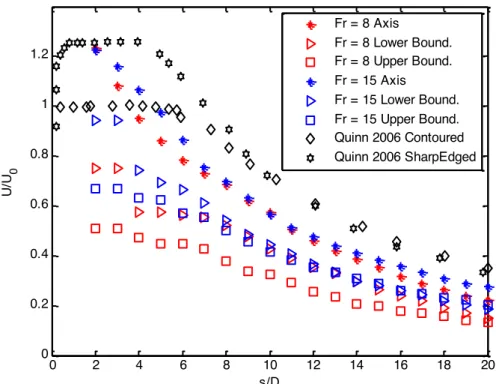
The mean centerline velocity decay UC/U0 versus the non-dimensional axial coordinate s/D for the two
simulated INBJs (colored asterisks) and for the simple jets simulated by Quinn, 2006, issuing from a sharp-edged (black stars) and a contoured (black rhombi) orifice, is shown in Figure 4. The INBJ centerline velocity decay values have a similar trend to the sharp-edged orifice ones, starting with values larger than one due to the vena contracta effect. Nonetheless, the INBJ velocity decay is higher, due to their higher widening with respect to the simple jet one. For the same reason, the obtained trend is steeper for the INBJ with Fr = 8 than for the one with Fr = 15. Moreover, Figure 4 shows the decay of velocity computed on the profiles perpendicular to the jet axis, at a value of r/D (the orthogonal to the axis non-dimensional distance from the axis) equal to the half widening of a simple jet (simple jet values used for this computations are taken from Quinn, 2006) for the lower (triangles) and upper (squares) regions of the INBJs. The highest velocities are located in the lower boundary, with a sudden decrease at around s/D = 4, which corresponds to the region where the inner core of velocity tends to move toward the upper region, as visible on Figure 2. The velocity at the upper boundary is almost constant until around s/D = 6, subsequently following a more gradual decay, without any sharp step. Finally, the velocities of the lightest INBJ (Fr = 15) are always higher than the ones of the heaviest INBJ, due to the fact that these values have been measured at the same orthogonal distance from the axis and, consequently, the values of the lightest INBJ (which widens more, see Figure 3) are closer to the high velocity core than the values of the heaviest one.
Figure 4. Streamwise non-dimensional mean velocity decay U/U0 along the axis (asterisks) and in the upper (squares)
and lower (triangles) region of the near-field of an INBJ with Re = 1000, q = 65° and different Fr (red: 8, blue: 15), and of two simple jets (Quinn, 2006; sharp-edged orifice: black stars; contoured orifice: black rhombi); the upper and lower
boundary decays are measured in correspondence to the widening of a simple jet.
5.2 Velocity second order statistics
0 2 4 6 8 10 12 14 16 18 20 0 0.2 0.4 0.6 0.8 1 1.2 s/D U/ U 0 Fr = 8 Axis Fr = 8 Lower Bound. Fr = 8 Upper Bound. Fr = 15 Axis Fr = 15 Lower Bound. Fr = 15 Upper Bound. Quinn 2006 Contoured Quinn 2006 SharpEdged
The Turbulent Kinetic Energy (TKE), non-dimensionalised by Umax2, fields for the two simulated INBJs are
presented on Figure 5; the jet axes (white lines) are the same of Figure 2. Figures 2a and 2b display similar and asymmetric behavior: TKE values are low close to the jet origin but, at a distance of few diameters from the origin, the onset of the Kelvin Helmholtz billows causes a sudden increase of TKE values. Two high value regions at the jet sides can be spotted, one located at the lower boundary, which occurs nearer to the orifice and is shorter and more intense with respect to the other one, located in the upper region, which presents lower but more persistent values. As the distance from the origin s/D increases, the lower TKE peak region is deflected toward the jet axis and the two peaks tend to merge into a single peak; going further, TKE tends to rapidly decrease as the INBJs become wider.
Figure 5. Map of the non-dimensional Turbulent Kinetic Energy TKE/Umax2 in the near-field of an INBJ with
Re = 1000, q = 65°, Fr = 8 (a) and 15 (b); the white line is the jet axis.
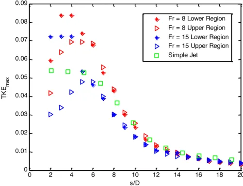
In Figure 6, the streamwise decay of TKEmax (i.e., the maxima of TKE/Umax2 computed on sections
orthogonal to the jet axis) in the upper (triangles) and lower (asterisks) region of the near-field of the two INBJs with Fr = 8 (red symbols) and Fr = 15 (blue symbols) and at the boundary of a simple jet (which is, of course, symmetric) with the same Re (green squares) are plotted versus s/D. This allows to better highlight the mentioned differences between the upper and lower region of an INBJ. All the curves show a similar trend, with an initial growth, a peak and a following decrease; moreover, the values in the lower region tend to be higher than the ones in the upper region, until around s/D = 6, where the upper region curve collapses into the lower region one. These higher values in the lower region are due to the local unstable stratification, with more intense velocity fluctuations due to the different directions of local momentum and buoyancy. The simple jet values tend to initially stay between the upper region and the lower region values, but showing a smoother trend, with a less pronounced peak, to then collapse, at a distance of around 10 diameters from the origin, to the INBJ values. However, it should be noticed that the asymptotic value of the simple jet tends to be higher than the INBJ ones, possibly suggesting that the higher initial turbulent fluctuations in INBJs tends to dissipate faster the TKE in this last case than in the simple jet one. This point seems to be strengthened by the data of Figure 7 and Figure 8, where the simple jets values always tend to an asymptote which is higher than the INBJ one.
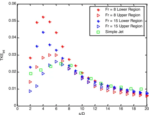
The streamwise decay of TKEint (i.e., the integral non-dimensional Turbulent Kinetic Energy TKE/Umax2) in
the near-field of two INBJs with Fr = 8 (red asterisks) Fr = 15 (blue asterisks) and of a simple jets with the same Re (green asterisks) is plotted in Figure 7 along the jet axis.
X/D Y/ D -2 0 2 4 6 8 10 12 0 2 4 6 8 10 12 14 16 18 0 0.01 0.02 0.03 0.04 0.05 0.06 0.07 0.08 X/D Y/ D 0 5 10 15 0 5 10 15 20 25 0 0.01 0.02 0.03 0.04 0.05 0.06 0.07 a b
Figure 6. Streamwise decay of the maximum non-dimensional Turbulent Kinetic Energy TKE/Umax2 in the upper
(triangles) and lower (asterisks) region of the near-field of an INBJ with Re = 1000, q = 65° and different Fr (red: 8, blue: 15) and of a simple jet with the same Re (green squares).
Figure 7. Streamwise decay of the integral non-dimensional Turbulent Kinetic Energy TKE/Umax2 in the near-field of
an INBJ with Re = 1000, q = 65° and different Fr (red: 8, blue: 15) and of a simple jets with the same Re (green).
The integrals are computed on profiles orthogonal to the jet axis, up to the half velocity jet widening above defined. The influence of Fr on this parameter is more clear: the values of INBJs always start higher than the ones of simple jet, with a more pronounced peak (with a higher value for the lower Fr which tends to decrease as Fr increases). The peak for the simple jet is found more streamwise if compared to the INBJ
0 2 4 6 8 10 12 14 16 18 20 0 0.01 0.02 0.03 0.04 0.05 0.06 0.07 0.08 0.09 s/D TK E m a x Fr = 8 Lower Region Fr = 8 Upper Region Fr = 15 Lower Region Fr = 15 Upper Region Simple Jet 2 4 6 8 10 12 14 16 18 20 0 0.01 0.02 0.03 0.04 0.05 0.06 0.07 0.08 0.09 s/D TK E in t Fr = 8 Fr = 15 Simple Jet
ones. Moreover, those initial higher values for the INBJs are followed by a higher asymptotic value of the simple jet, in confirmation to what previously stated for TKEmax.Finally, TKEint is separately measured at the
upper (triangles) and lower (asterisks) region of the two INBJs with Fr = 8 (red asterisks) and Fr = 15 (blue asterisks) and at the boundary of a simple jet (which is, of course, symmetric) with the same Re (green squares) and plotted versus s/D in Figure 8. The difference with Figure 7 is that the integrals are computed on profiles orthogonal to the jet axis, up to the half velocity jet widening, only from the axis upwards or downwards. As observed in Figure 6, the highest values are measured in the lower region and data finally collapse, with the simple jet values that tend to remain in the middle between the upper and lower region values; moreover, the asymptotic value for the simple jet is higher than the INBJ ones.
Figure 8. Streamwise decay of the integral non-dimensional Turbulent Kinetic Energy TKE/Umax2 in the upper
(triangles) and lower (asterisks) region of the near-field of an INBJ with Re = 1000, q = 65° and different Fr (red: 8, blue: 15 and of a simple jet with the same Re (green squares).
5.3 Velocity third and fourth order statistics
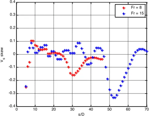
We have separately analyzed the streamwise (i.e., tangential to the jet axis) velocity component from the spanwise (or radial, i.e. orthogonal to the jet axis) one to highlight their influence on the velocity distribution of INBJs. We show here some preliminary results of this analysis, highlighting that the maximum elevation of the two INBJs investigated here is found at s/D ≅ 22 for Fr = 8 and at s/D ≅ 40 for Fr = 15; this because the point of maximum elevation plays a relevant role in the physics of INBJs.
In Figure 9 we show the streamwise evolution of the non-dimensional streamwise velocity skewness
Vs skew/Umax3 for two INBJs with Re = 1000, θ = 65° and different Fr (red asterisks 8, blue ones 15). Vs skew
starts from very low values close to the jet origin (so Vs has a distribution with the heaviest tail on the left,
which corresponds to the upper region of the jet), then it grows and tends to stabilize around zero with small oscillations (between +0.1 and -0.1, so close to a symmetrical distribution, even if never being fully symmetrical). When the INBJs reach their maximum high, Vs skew is fairly zero (Vs has a symmetrical
distribution) but become negative after a short distance and experience the lowest value when the jets are in their descending branch, to then return to an almost symmetrical distribution; this is a consequence of the strong mixing that the jet experiences after the point of maximum elevation, because of the interaction between the upward and downward branches before mentioned. This behavior seems to be deeply different from the one of simple jets, investigated by Hashiehbaf and Romano (2013) for sharp hedged circular simple
0 2 4 6 8 10 12 14 16 18 20 0 0.01 0.02 0.03 0.04 0.05 0.06 s/D TK E in t Fr = 8 Lower Region Fr = 8 Upper Region Fr = 15 Lower Region Fr = 15 Upper Region Simple Jet
jets, which seem to reach, after some oscillations, a symmetrical distribution at a short distance from the origin.
Figure 9. Streamwise evolution of the non-dimensional streamwise velocity skewness Vs skew/Umax3 for two INBJs with
Re = 1000, q = 65° and different Fr (red: 8, blue: 15).
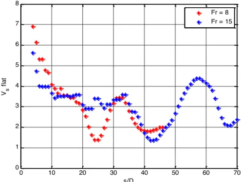
In Figure 10 we show the streamwise evolution of the non-dimensional streamwise velocity kurtosis
Vs flat/Umax4 for two INBJs with Re = 1000, θ = 65° and different Fr (red asterisks 8, blue ones 15).
Vs flat/Umax4 starts from very high values (i.e., larger than 3 for a Gaussian distribution), highlighting a peaked
distribution of Vs corresponding to a strong velocity core. Afterwards, kurtosis tends to decrease until its
minimum value, reached after a short distance s/D from the jet maximum high for the two INBJs. After this point, Vs flat/Umax4 tends to oscillate around 3, showing that the streamwise component of the velocity would
tend to become Gaussian if the INBJs would have more space to develop. As stated before for the skewness, INBJ behavior seems to be quite different from the one of simple jets (Hashiehbaf and Romano, 2013) that tend to achieve a Gaussian distribution.
In Figure 11 we show the streamwise evolution of the non-dimensional spanwise velocity kurtosis
Vr flat/Umax4 for two INBJs with Re = 1000, θ = 65° and different Fr (red asterisks 8, blue ones 15). The
behavior of the spanwise component is opposite to the streamwise one: very low values close to the origin, highlighting a tailed distribution of Vr, which tend to grow until their maximum, at the s/D almost equal to
the one of the jet maximum high, to eventually decrease and tend to oscillate around a value (approximately 1.5) which is much lower than the value of 3 typical of a Gaussian distribution. Hence, except for the peculiar maximum close to the jet maximum high, a strongly non Gaussian behavior characterizes the whole INBJ evolution.
Bearing in mind what previously shown for the Vs, we can suppose that in the downward branch of INBJs
the streamwise velocity components tend to a symmetrical Gaussian distribution (without reaching it), whilst the spanwise velocity components have a more heavy tailed distribution.
0 10 20 30 40 50 60 70 -0.4 -0.3 -0.2 -0.1 0 0.1 0.2 0.3 0.4 s/D V s s k e w Fr = 8 Fr = 15
Figure 10. Streamwise evolution of the non-dimensional streamwise velocity kurtosis Vs flat/Umax4 for two INBJs with
Re = 1000, q = 65° and different Fr (red: 8, blue: 15).
Figure 11 Streamwise evolution of the non-dimensional spanwise velocity kurtosis Vr flat/Umax4 for two INBJs with
Re = 1000, q = 65° and different Fr (red: 8, blue: 15).
6. Conclusions
The behavior of the Inclined Negatively Buoyant Jets, released from a sharp-edged orifice, was investigated in the laboratory using a novel technique to measure the velocity fields, namely Feature Tracking Velocimetry, in order to study, among the others, their dependence on the densimetric Froude number. Statistics of the velocity fields, from the first to the fourth order, of jets with different densimetric Froude numbers were used to characterize the Inclined Negatively Buoyant Jet behavior and their difference from
0 10 20 30 40 50 60 70 0 1 2 3 4 5 6 7 8 s/D V s fl a t Fr = 8 Fr = 15 0 10 20 30 40 50 60 70 0 0.5 1 1.5 2 2.5 3 3.5 4 s/D V r fl a t Fr = 8 Fr = 15
Simple Jets.
The analysis of mean velocity fields highlights the different behavior of Inclined Negatively Buoyant Jets with respect to Simple Jets, but only at a certain distance from the outlet. On the contrary, velocity second order statistics already unveil the lack of axisymmetry at a very short distance from the jets’ origin. This seems to be an outcome of the strong non-Gaussianity of the radial component of the velocity, as shown by the higher order statistics along the jet axis. This implies that the asymmetry and non-Gaussianity are key features of Inclined Negatively Buoyant Jets that cannot be neglected even in their near field, oppositely to what previously stated in literature.
Moreover, the analysis of the second order statistics of the velocity highlights a dependence of the features of sharp-edged orifice jets on the densimetric Froude number.
List of References
• Avanzini C. (2006) An outline of common practical problems and solutions in the diffusers design, Proc. 4th Intl. Conf Marine Waste Water Disposal and Marine Environment & 2nd Intl. Exhibition Materials, Equipment and Services for Coastal Waste Water Treatment Plants, Outfalls and Sealines Antalya, Turkey, Mem Ajans, Istanbul.
• Besalduch L.A., Badas M.G., Ferrari S., Querzoli G. (2013) Experimental Studies for the characterization of the mixing processes in negative buoyant jets, European Phis. J. W.o.C., 45, art. no. 01012.
• Besalduch L.A., Badas M.G., Ferrari S., Querzoli G. (2014) On the near field behavior of inclined negatively buoyant jets, European Phis. J. W.o.C., 67, art. no. 02007.
• Cipollina A., Brucato A., Grisafi F., Nicosia S. (2005) Bench scale investigation of inclined dense jets, J. Hydraulic Eng., 131(11), 1017-1022.
• Falchi M., Querzoli G., Romano G.P., (2006) Robust evaluation of the dissimilarity between interrogation windows in image Velocimetry, Exp. Fluids 41(2), pp 279-293.
• Ferrari S, Querzoli G. (2010) Mixing and re-entrainment in a negatively buoyant jet, J. Hydraulic Research, 48(5), 632-640.
• Hall N., Elenany M., Zhu D., Rajaratnam N. (2010) Experimental Study of Sand and Slurry Jets in Water, J. Hydraul. Eng., 136(10), 727–738.
• Harris C., Stephens M.A. (1988) Combined corner and edge detector. In: Proceedings of the 4th Aivey Vision Conference, Manchester, 147-151.
• Hashiehbaf A., Romano G.P., (2013) Particle image velocimetry investigation on mixing enhancement of non-circular sharp edge nozzles, Int. J. Heat Fluid Flow, 44, 208-221.
• Koh R.C.Y., Isaacson M.S., Brooks N.H. (1975) Plume Dilution for Diffusers and Multiport Risers, J. Hydraulic Eng., 109(2), 100-220.
• Lai, C.C.K. & Lee, J.H.W. Mixing in inclined dense jets in stationary ambient. Journal of Hydro-environment Research, 6, 9-28, 2012.
• Lindberg W.R., Petersen J.D. (1991) Negatively buoyant jet (or plume) with application to snowplow exit flow behaviour, Transportation Res. Record,1304, 219–229.
• List E.J (1979) Turbulent jets and plumes. In: Fisher H.B., List E.J., Koh R.C.Y., Imberger J., Brooks N.H. (Eds) Mixing in inland and coastal water, New York, USA, Academic Press.
• Mi J., Nathan G.J., Nobes D.S. (2001) Mixing characteristics of axisymmetric free jets from a contoured nozzle, an orifice plate and a pipe, J. Fluid Eng. ASME 123(4), 878-883.
• Mi J, Kalt P., Nathan G.J., Wong C.Y. (2007) PIV measurements of a turbulent jet issuing from round sharp-edged plate, Exp. Fluids 42(4), 625-637.
• Roberts P.J.W., Ferrier A., Daviero G. (1997) Mixing in inclined dense jets, J. Hydraulic Eng. 123(8), 693–699.
• Wright S.J., Wong D.R., Zimmerman K.E., Wallace R.B. (1982) Outfall diffusers behaviour in stratified ambient fluid, J. Hydraulics Div. ASCE 108(HY4), 483–501.
• Quinn W.R. (2006) Upstream nozzle shaping effects on near field flow in round turbulent free jets, European Journal of Mechanics B/Fluids 25 279–301.