Fiscal Implications of Pension Reforms in Italy
Agar Brugiavini
University “Ca’ Foscari” of Venice
Franco Peracchi
1. Introduction
A “good” pension reform should address a number of issues. One important aspect is the financial soundness of the system, particularly in the light of the legacy that we leave to future generations. Policy makers should also address economic efficiency at two levels: no waste of resources for a given contribution rate (or for a given benefit level), and no distortions of individual choices (or at least minimize distortions). The main distortions associated with a pension system or with its reform have to do with saving and labor supply behavior.
Italy has seen a flurry of reforms during the 1990s, and economists and policy makers are still struggling to assess the results and the long-term effects of these reforms. Many analysts argue that the overall design of the recent Italian reforms is probably a good one, and yet more steps need to be taken to speed up the reform process and reap the benefits which, due the adverse demographic trends, could easily evaporate.
In this paper, we contribute to the current debate on the Italian pension system by analyzing the impact of social security reforms, in terms of both budgetary implications and distributional effects. This is done by simulating the effects of three hypothetical reforms, plus the effects of the 1995-reform of the Italian pension system (the so-called Dini reform). Our approach relies on the use of a semi-structural econometric model to predict retirement probabilities under different policy scenarios, so as to properly take into account the
behavioral effects of the reforms. On the basis of the estimated retirement model, we develop a complete accounting exercise which includes not only changes in gross future benefits due to policy changes, but also changes in social security contributions, income taxes and value added taxes. Thus, our results provide not only estimates of the workers’ gains or losses, but also an exhaustive evaluation of the gains and losses for the government budget.
We find that the reforms, particularly the Dini reform (once fully phased in), have a substantial impact on individuals’ retirement decisions and their net social security wealth, as well as substantial gains for the government finances.
2. An overview of the Italian pension system and its reforms
Before turning to the analysis of different social security reforms, it seems useful to briefly describe the reform process which has taken place in Italy, and the recentdevelopments in the political arena. The growing concern of the European Union with meeting the targets imposed by the Stability and Growth Pact has contributed to develop a debate on the effects of the recent reforms and the need for further reforms. It should be mentioned that Italy, along with the other member states of the EU, committed itself to increase the effective retirement age of 5 years by the year 2010. Specific targets have also been set on participation rates of older workers.
Many argue that the changes of the 1990s may be inadequate in the light of future demographic trends, and that it is imperative to raise the effective retirement age. Empirical work carried out on the issue shows that there is a strong relationship between the tax incentives to retire and the age at which men are observed to retire in different countries4. For Italy, we still observe a substantial number of early retirees.5 Therefore, an evaluation of the impact and efficacy of the reforms, which has already started with a Ministerial Committee6 appointed by the Italian Welfare Ministry, is of crucial importance.
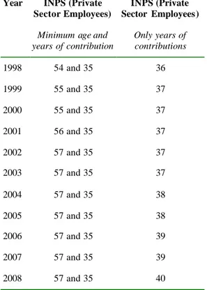
The reforms of the 1990s have tackled several aspects of the Italian social security system, but three are particularly relevant: (i) benefit computation rules; (2) indexation rules, and (3) retirement age and eligibility criteria.7 It is useful to recall that the vast majority of the population is insured with the National Institute for Social Security (INPS), and since this paper focuses attention on the most important fund administered by the INPS, the Private Sector Employees Fund (FPLD, our description of the reforms will mainly focus on the changes taking place for private sector employees.
A first reform (known as the Amato reform) was passed by Parliament in 1992. Once phased in, it would reduce pension outlays and iron out major differences between various sectors and occupations. However, this reform changed only marginally the rules governing early retirement and, according to many, did not produce the much needed savings in the budget. Hence the second reform (the so-called Dini reform) of 1995.This reform totally changed some of the basic rules for granting benefits to future retirees and tried to harmonize the actuarial rates of return for early and late retirees. Table 1 summarizes some of the key features of three regimes: the regime prevailing before the Amato reform (denoted as Pre-1993 regime) , the one prevailing during the transition (currently in place), and the one prevailing with the Dini reform fully in place (post-1995-Regime). However both the Amato and Dini reforms are characterized by a very long transitional period affecting all the cohorts
4 The concept of an “implicit tax” was introduced by Gruber and Wise (1999). 5 See Brugiavini and Peracchi (2001) and Brugiavini, Peracchi and Wise (2001).
6 Relazione Finale della Commissione Ministeriale di “Verifica del sistema previdenziale ai sensi della
legge 335/95 e successivi provvedimenti, nell’ottica della competitività, dello sviluppo e dell’equità”, October 2001.
7 For a description of Italian social security system before 1992 , see Brugiavini (1999), Brugiavini and
of post-1992-retirees: the provisions for the transitional periods involve a pro rata method of establishing eligibility and benefit computation criteria on the basis of seniority.
2.1 The Dini reform and recent assessments of the reform
process
The Dini reform adopts a defined-contribution method of benefit calculation. The first benefit is the annuity equivalent to the present value (at retirement) of past payroll taxes, capitalised by means of a 5-years moving average of nominal GDP growth-rates. The relevant payroll tax rate is 33% and an age-related actuarial adjustment factor is applied to the resulting figure.8 In this case too, capping is applied (on the present value of contributions, rather than on pensionable earnings). The 1995 ref orm introduced – at the steady state - a window of pensionable ages with an associated actuarially-based adjustment of pensions. This window goes from age 57 to age 65, with “actuarial adjustment factors” of 4.720% and 6.136% respectively. These coefficients, which make the present value of future benefits equal to capitalised contributions, can be revised every ten years on the basis of changes in life expectancy and a comparison of the rates of growth of GDP and earnings assessed for payroll taxes. It should be noted that, even at the steady state, the system will not achieve complete age-neutrality given the mortality prospects of Italian workers.9
Minimum contribution requirements changed from the initial 15 years, to just 5 years after 1995. Payroll taxes increased to 32.7% of gross earnings (to be split between employer and employee) from approximately 27% in 1995.
The implementation of the reform was (and still is) extremely gradual. Workers with at least 18 years of contributions in 1995 will rec eive a pension computed on the basis of the rules applying before 1992. Those with less than 18 years of contributions in 1992 will be subject to a pro- rata regime: the 1995 reform will apply only to the contributions paid after 1995. 10 Only individuals be ginning to work after 1995 will receive a pension computed only on the basis of the new rules. Hence the length of the transition phase, and other aspects of the reform, may significantly reduce its expected benefits.
A first round of evaluations of the reforms became available throughout the 1990s. Some of these evaluations were based on “generational accounting”. For example, it was
8
Hence the benefit is: (33%)*(adjustment factor)*(present value of SS taxes).
9
See Barbi (2001)
10 The benefits paid to individuals in the pro-rata regime will be computed on the basis of
estimated that in order to ensure the long-term sustainability of public finances, a 5% increase in the taxes paid by all generations would be required. Without the pension reforms introduced in the 1990s, the required tax increase would have been 9%. About 40% of those employed in 1999 could fully retire under the pre-1992 regime. For these people, the incentive to retire early was even increased by the expectations that retirement conditions might be tightened (Franco, 2002).
The Report of the Ministerial Committee published in the year 2001 shows that the savings obtained between 1996 and 2000 are essentially due to changes in the indexation rules and curtailing early retirement. The difficulty in building a complete evaluation model, that incorporates behavioural responses to the reforms, relies on the availability of good data and on the overall approach. Brugiavini and Peracchi (2001) provide an econometric model which focuses on dynamic incentives but does not address fiscal implications, while other recent studies 11 carry out accounting exercises that neglect the impact of policy changes on the retirement decisions of individuals.
3. The retirement model
The simulation exercise carried out in the present paper relies on an econometric model of the retirement decision of Italian workers largely based on the work of Gruber and Wise (2001) and already applied to the Italian case by Brugiavini and Peracchi (2001). In the present paper we limit our description of the econometric work to the main features of the modeling strategy and to the data. An important difference with respect to Brugiavini and Peracchi (2001) is the fact that the availability of a new release of the data, characterized by a larger sample size, allows us to follow a novel approach. Therefore the underlying empirical work deserves some attention also in this paper.
3.1 The data
The retirement decision is analyzed through a reduced form model estimated on a random sample of administrative records from one of the INPS archives12. The sample is drawn from the so-called INPS Workers-Archive (Archive O1M), which contains records on all private sector employees ensured with INPS. The information on each employee is filed in by the
11
See Ragioneria Generale dello Stato, 2001 and Fornero-Castellino, 2001
12
This is a sub-sample of workers borne either on March 1st or on October 1st of any possible year contained in the Archive .
employer on a standard form containing a small number of entries. We have a random sample of these employees in the form of a panel covering a period of about 20 years from 1973 to 1997. The sample contains 200,000 workers entering the archive at any time during the period considered. Employment spells can last any number of years, and individuals can leave the sample and enter again in any subsequent year. The panel is therefore highly unbalanced. The main advantages of using these data are that they span a fairly long time period and contain information on gross earnings, which form the basis for the calculation of social security benefits. However, there are several shortcomings.
(1) The data set only covers private sector employees, leaving out public sector employees and the self-employed. Even for private sec tor employees, however, coverage is not full and a small fraction of them is not included.
(2) The reason for a worker dropping off the archive is not known: in addition to retiring, workers could die, become self- employed or public sector employees, or simply stop working.
(3) Important covariates (e.g. education level, spousal information and other family background variables) are missing. As a result, we have very few demographic controls available, we do not know about marital status, and cannot say muc h about differential mortality.
(4) There is no information on receipt of disability or other types of benefits.
The initial sample selection, carried out in order to estimate suitable earnings histories, is as follows. We focus on workers between 18 and 70 years of age. We drop observations for which one important indicator (such as age) is missing and individuals who work less than 26 days a year. We also exclude from the analysis workers belonging to special INPS funds (nursery school teachers, local authorities employees, etc.)13.
3.2 Earnings projection and transitions to retirement
In order to estimate earnings profiles and eventually measure social security wealth, we further select the sample by including only workers who are present in the sample for an uninterrupted period of at least five years (workers often appear for one year and then disappear from the sample for a long spell). The 5-year minimum requirement is motivated by the fact that this corresponds to the minimum contributive period under the 1995 reform. We only keep workers who do not have substantial gaps (more than 10 years missing) in their records. This is because we cannot say whether in that time span they were engaged in other labor market or non-labor market activities (such as maternity leaves, or undertaking further
education). The choice of a 10-year interval is arbitrary and is based on a preliminary inspection of the data14.
The information available in order to model age-earnings profiles in the INPS sample consists of age, gender, occupation, sector of employment and region of working activity15.
The specification of a model for the age-earnings profile represents an essential step in the estimation of social security wealth at the individual level. This is especially important in Italy, as the process of social security reform involves moving from a “final salary” type of benefit formula (pre-1993 system) to a formula based on the value of lifetime contributions (1995 reform).16 Below we describe additional hypothetical reforms, which also involve extending the benefit calculation period.
The earnings -modeling strategy is as follows: individual real age-earnings profiles are modelled with individual fixed effects in order to fill gaps of one or two years in workers’ career. The profile is assumed to be completely flat after the last year of observed earnings. This corresponds to the assumption that, at the individual level, the real earnings process is a random walk with no drift. In practice, the “jump-off” point for the earnings projections is taken to be the average of the last three years of observed earnings. This jump-off point pins down the level of the age-earnings profile for each individual.17 Note that this might seem to underestimate future earnings growth, particularly for younger cohorts, but since our “sample at risk” (as defined below) consists mainly of older cohorts, the problem may not be too severe18. Furthermore, for ages above 50, earnings are lower on average and very noisy, possibly because of part-time work or the coexistence of early retirement benefits and working activities. When going backward, using a flat earnings profile would grossly 13 We could include these observations to add variability across funds, but these workers represent only
a small number (less than 100 observations) and tend to exhibit many gaps in their careers.
14 It should be noted that, in order to gain variability in social security benefits, we did experiment with
a larger sample including almost all workers, regardless of the existence of gaps in their careers. However, this did not add valuable information as the majority of workers with substantial spells out of the private sector would end up qualifying for minimum benefits (the level of which is fixed by legislation each year) or for an old age income guarantee (pensione sociale). Hence there would be very little correlation between earnings histories and pension benefits for these individuals, and the effects of potential reforms in changing the incentives to retire would be negligible (these workers would basically qualify for the minimum benefit under all regimes). Therefore these cases would end up blurring the results rather than adding variability to be exploited. Finally, our choice of the ten years threshold and the requirement of a minimum of five years presence in the archive give us an estimated sample percentage of minimum benefit recipients which is not too far from what observed in the universe of pension awards as recorded by the INPS Administration (see Table 2.4).
15
This is actually the region where the firm is located. Hence a comparison with the SHIW and national accounts data reveals that there seems to be a higher number of workers located in the North-West, where many large firms have their headquarters.
16
In this and in the following sections we only describe results for the 1995 reform, results for the other cases are available on request from the authors.
17 When going backward, the jump-off point corresponds to the average of the first three observations
overestimate the level of earnings at earlier ages and grossly underestimate real earnings growth. To avoid this problem, individual earnings are assumed to grow at the annual growth rate of aggregate earnings, for the years when this information is available, and at a constant real rate of 1.5% otherwise.19
Notice that our first data point is in 1973, while we need to go back to the 1930’s for some of our workers in order to complete their working history. Hence, we would be forced to use a procedure which makes use of aggregate growth rates when projecting backwards into the distant past. Also, in projecting earnings forwar d, individuals are assumed to form expectations by “using the model”. In other words, for each age we only use actual earnings up to that age, and project earnings from that age forward according to the forecasting model.
At the moment we have no information on the reasons for which workers leave the archive. Thus, in order to use these data we have to make the strong assumption that every exit from the archive is due to retirement. In fact, rather than retiring, a worker could have died, or moved from private sector employment to public sector employment or to self-employment. Our identifying assumption is that, over the range of ages that we consider (from age 50 to 65), exit from the INPS archive is due to retirement and not to other reasons. This assumption is not in contrast with what we observe in an alternative sample provided by the Bank of Italy (Survey of household income and wealth-SHIW), where we have available the full set of information concerning the occupational status of individuals in each year 20. As for mortality, in the simulation we will purge the exits of the component which we can impute to the probability of death by age, sex and cohort.
For Italian workers, the only relevant alternative escape route from the labor force could be via disability. Many other bridging plans exist, but they would all fall in the category of “pre-retirement” or “early-retirement” and, in our data, they would effectively correspond to retirement. We argue that these exits via disability are non particularly relevant in our sample because, after the changes legislated in 1984, their importance as an escape route has greatly diminished and in the age range that we consider (50 to 70), the number of disability pensions is negligible relative to old age pensions21.
18
The cohorts at risk are defin ed according to year of birth: for the oldest cohort these are between 1918 and 1926, for the next cohort 1927-1936 and for the youngest cohort 1937-1944.
19 Aggregate earnings are equal to the earnings series put together by Rossi, Sorgato and Toniolo
(1993) for the years before 1970 and to national account statistics for subsequent years up to 1999.
20In the SHIW sample different definitions of pensioner are available, based on self-reported occupational status,
on earnings and on benefits receipts. However no marked difference in the distribution of retired people by age emerged from adopting different definitions.
21
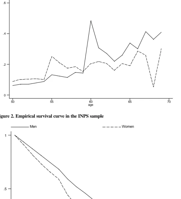
Figure 1 presents the non parametric retirement hazard based on the INPS sample for men and women. For men there is an important spike at age 60, but the hazard is not flat at younger ages, whereas for women there are several important ages at which the conditional probability of leaving the labor force peaks.
3.3 Definition of social security wealth and incentive
measures
Key ingredients of the econometric model are two concepts: the social security wealth and related dynamic incentives. It is useful to briefly recap these concepts.
For a worker of age a, we define social security wealth (SSW) in case of retirement at age h ≥ a as the expected present value of future pension benefits
∑
= +=
S h s s s hB
h
SSW
1)
(
ρ
,where S is the age of certain death, ρs = βs−aπs is a discount factor that depends on the rate of time discount ß and the survival probability πs at age s conditional on being alive at age h, and B(h) is the pension benefit expected at age
s
≥
h
+
1
in case of retirement at age h. Pension benefits are net of income taxes. Given the SSW, we define three incentive measures for a worker of age a.1. Social security accrual (SSA) is the difference in SSW from postponing retirement from age a to age a+1
[
( 1) ( )]
1 1( ) 2 1 SSW B a B a B a SSW SSA a a S a s s s s a a a + + + = + − = + − − =∑
ρ ρ .The SSA is negative if the expected present value of pension benefits foregone by postponing
retirement by one year is greater than
∑
[
]
+ = − + S a s s s s B a B a 2 ) ( ) 1 (
ρ , the expected present value
of the increment in the flow of pension benefits. The rescaled negative accrual
1
/
+−
=
a aa
SSA
W
τ
, whereW
a+1 are expected net earnings at age a+1 based on the information available up to age a, is called the implicit tax/subsidy of postponing retirement from age a to age a+1.2. Peak value:
PV
a=
max
h(
SSW
h−
SSW
a)
, h = a+1,..,R , where R is the mandatory retirement age (the latter does not exist in Italy, but given the retirement evidence we find it reasonable to put R = 70). Thus, the peak value is the maximum difference in SSW between retiring at future ages and retiring at the current age.3. Option value:
OV
a=
max
h(
V
h−
V
a)
, h = a+1,…, R, where[
]
γ ρ∑
+ = = S a s s s a k B h V 1 ) (is the intertemporal expected utility of retiring at age a, while
[
]
γ γ ρ ρ∑
∑
+ = + = + = S h s s s h a s s s h W k B h V 1 1 ) (is the intertemporal utility of retiring at age h > a. Thus the option value is the maximum utility difference between retiring at future ages and retiring at age a. We parameterize the model by assuming γ = 1 and k = 1.25. Under these assumptions,
V
a=
1
.
25
SSW
a andh h a s s s h W SSW V 1.25 1 + =
∑
+ = γ ρ .If expected earnings are constant at
W
a(as assumed in our earnings model), then) ( 25 . 1 1 a h h a s s a a h V W SSW SSW V − =
∑
+ − + = ρThat is, the peak value and the option value are proportional to each other except for the effect due to the term
∑
h= +a s 1
ρ
s .In the actual calculation of SSW we assume a real discount factor of 1.5 percent (β = .985). Benefits are defined in real terms and the indexation rules prevailing under each legislation are implemented (e.g. in the baseline we apply indexation to both price inflation and real wages). We also assume that real earnings growth after 1997 (the last year of the INPS sample), is constant at 1.5%.
Estimation of SSW is carried out separately for men and women. Household social security wealth is obtained simply as the man’s social security wealth when the wife does not work. In estimating the model, we also had to deal with the fact that the actual age of entry into the labor market is not always known. We used the information on the initial occupational level to get a reasonable proxy for educational attainments. This was then used to impute an initial age for the worker’s contributive history.
Eligibility rules and benefit computation rules prevailing under each regime are rather complex (see Section 2), and some shortcuts were made. Finally, we computed social security wealth net of income tax, by subtracting from gross pension benefits income taxes as due.
3.4 The reduced form retirement model: methodology and
estimation results
In this section we present the results of modeling exit into retirement using probit models that include, in addition to a standard set of covariates (such as age, occupation and sector), the incentive measures discussed in the previous section.
The response variable is a binary indicator, representing exit from the INPS sample between the year t and the year t +1. The population at risk consists of workers aged between 50 and 70 in any of the relevant years. The sample used for es timation includes all consecutive pairs of years from 1980-1981 through to 1996-1997. We restrict the analysis to individuals at risk after 1980: the reason is twofold. First, it is very hard to capture the behaviour of workers taking into account all the institutional changes affecting the various cohorts over a long time span. An advantage of the period between 1980 and 1992 is that it is a relatively stable period in terms of policy changes. Second, because in some cases we have to model earnings profiles going back fifty years, given the existing limitations on aggregate wage data it is reasonable to limit the time horizon to recent years. In this way, our oldest worker is aged 70 in 1980 and we only need to back-cast earnings to the year 193022.
The social security regime is assumed to be the transitional one introduced in 1992 (see Table 1). This is the relevant regime for the workers in our sample, who would not yet experience the changes introduced by the 1995 reform through the sample period. Overall, using the pre- 1993 rules instead, would lead to negligible differences in terms of social security wealth and eligibility. This is because, as already mentioned, the rights of workers near retirement were changed only marginally by the 1992 reform: according to seniority, most workers at risk would fully retire under the pre-1993 rules.
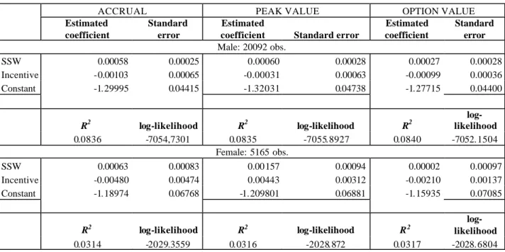
For each incentive measure, two basic specifications are considered, for a total of six estimated models. The incentive variables are: the accrual, the peak value and the option value whereas the dependence of the retirement hazard on age is modelled either through a simple linear age term or through a full set of age dummies. All specifications include a set of sectoral and regional indicators and a set of earnings measures relevant for the retirement choice. Differently from our previous work and from other countries which contribute to the
project, we only use two “resource” measures capturing the level of social security wealth and the trade off between benefits and labor earnings: net social security wealth and pensionable earnings respectively23. The additional variable measuring future earnings, which we included in previous studies, is left out because, in the Italian case, a multicollinearity problem emerges under the baseline and the transitional period24. The problem is caused by the way benefits are computed: pensionable earnings, which form the basis of our social security wealth estimate, are the average of the last five years earnings, and in many cases this takes the same value of (or a very close value to) one-step-ahead projected earnings.
Results for the specification with age dummies are summarized in Table 3: each column refers to a particular incentive variable and we report only the estimated coeffic ients of the variables of interest. It should be noted that the purpose of the estimation here is not to produce a “good fit”, but rather to create a basis for the simulation exercise by adopting a parsimonious specification25. The use of age dummies increases the fit relative to the model with a linear age term, but only marginally. This suggests that age is an important determinant of retirement decisions but, despite the presence of spikes in the hazard, we get only marginal gains by making use of a fully parameterized model. Hence, these spikes may be less important than it first appears in explaining the age-retirement process, as most of the action comes from the exits taking place between age 50 and age 60. As shown in Table 3, the social security wealth variable and the incentive variables are, by and large, of the correct sign: of the incentive variables the accrual and option value have the correct sign and are significantly different from zero.
4. Simulating Policy Changes
The aim of this section is to simulate the total fiscal implications of pension reforms. The hypothetical reforms, designed as described below, contain some useful elements for the debate currently taking place in Italy. For example the reform which we indicate as “actuarial
22 Retirement is not mandatory. Given that we assume an individual at risk up to age 70, and given that
we cannot exclude that she started working at age 20, we cannot rule out the possibility that this individual worked for fifty years.
23 T obe more precise we use a quadratic polynomial polynomial in pensionable earnings. All
continuous variables enter in the form of deviation from the mean.
24 For brevity we do not report the estimates of regressions of the future earnings variable against social
security wealth, pensionable earnings and all the relevant covariates. This regression shows the clear symptoms of multicollinearity, e.g. an extremely high t-statistics for the two variables under investigation.
25
adjustment” represents a change of the current Italian system which many experts and policy makers advocate. We also simulate the steady state effects of the actual reform introduced in 1995 (the so-called Dini-Reform).
4.1 Social security regimes
The baseline (R0) , i.e. the reference regime, is the social security system prevailing before 1992 and the various regime changes are evaluated against this regime26. As for the reforms considered it is useful to provide a brief description.
R1: Age Shift. This reform preserves all the features of the system but increases by three
years the normal retirement age. Since in Italy all ages before the normal retirement age are potentially an early retirement age (conditional on seniority) the entire hazard is effectively shifted by three years. The seniority rule is preserved in its original format (see also Table1).
R2: Actuarial Adjustment. This reform should achieve an actuarially fair system without
changing any other feature of the program (i.e. no change in basic benefit calculation rules, in means-testing and eligibility to minimum benefits and in indexation). The normal retirement age is the same as for the base case and the rules in place are unchanged at that age (hence, the replacement ratio is the same at that age). The reform introduces an actuarial adjustment of 6% for each year away from the normal retirement age. Thus, benefits becoming available before the normal retirement age receive a cut of 6% per year, while benefits becoming available after the normal retirement age are increased by 6% per year.
R3: Common Reform. This reform is common to all countries considered in this volume. The
crucial feature is that, differently from the other cases, this reform envisages an ideal system, which represent a complete departure from the systems currently in place in many countries (Italy is one example) and is the same for all countries. This simulation features an early retirement age of 60 and a normal retirement age of 65. It provides a retiree with a benefit, which replaces 60% of her projected earnings when she turns 65. It applies an actuarial reduction of 6% per year for early claiming and an actuarial increase of 6% per year for later claiming. It essentially makes early retirement costly and introduces age-neutrality in retirement choices.
26
As we already pointed out the econometric model which predicts retirement is estimated on the sample of workers observed between 1974 and 1997, hence experiencing the transitional period. In the estimation we evaluate social security wealth and the incentive variables according to the rules of the
R4: The 1995 Reform . The 1995 reform adopts a notionally defined contribution method of
benefit calculation. The first social security benefit is the annuity equivalent to the present value (at retirement) of past payroll taxes, capitalised by means of a 5-years moving average of the nominal GDP growth-rate. The 1995 reform introduced – at the steady state - a window of eligible ages with actuarially - based adjustment of pensions. These vary between age 57 and 65 with “actuarial adjustment factors” between 4.720% and 6.136% respectively27. Capping is applied (on the present value of contributions rather than on pensionable earnings).
4.2 Simulation methodology
For each of the five policies described above (four regime changes plus the baseline), we have estimate, for each worker in the sample of interest, of the social security wealth variable, of the incentive measures. For each worker we also observe a number of covariates such as age, occupational status, etc. We simulate retirement decisions of these workers on the basis of the econometric model described in Section 3 above, using the social security wealth variable and of the incentive measures specific to each regime. All other covariates are identical across simulations. In this way, retirement probabilities change in response to changes in the policy variables according to the estimated parameters (also shown in Table 3). However, a few adjustments are needed in order to adapt the estimates to the policy environment. One of these adjustments concerns the age dummies. To recap we make use of two econometric models: one where age enters the specification linearly and is not affected by the reform changes (S1), and one where age effects are modelled through a set of age dummies (S3). The coefficients on the age dummies of this model are bound to be affected by the reforms over and above the changes implied by any modification in eligibility rules. For example in Italy the hazard for men has a spike at age 60, which is the normal retirement age for men under the baseline (R0). If the normal retirement age is shifted by three years (regime R1) then the age effect observed at age 60 should be felt at age 63, and the whole hazard should reflect the policy change.
Simulations are carried out in two steps: the first step generates retirement probabilities under the different scenarios, whereas the second step computes the fiscal implications of the changes. In order to carry out the exercise we initially focus on an homogeneous group of
transitional phase, because these are the incentives actually faced by individuals. However in the simulation we look at changes occurring between steady states.
workers by drawing from the original INPS sample a simulation sample of 699 individuals (men and women) born in 1938, 1939 and 194028. We disregard time differences between these three cohorts and simply take everybody to be of age 50 in 1990. For these individuals we have all the relevant information for all ages between 50 and 70, that is we follow the individuals through these ages even if some of them have effectively retired in the original sample. The intuition behind this procedure is to compute the direct fiscal effects of the reforms (the “mechanical effects”) and the fiscal effects due to changes in retirement behaviour (the “behavioral effects”) as seen from the perspective of an individual who reaches age 50 in 1990 and is considering whether to retire at any future age.
4.3 Basic Assumptions
Unlike most other countries in this project, we assume that men are married to a woman who does not work, while working women are single. Hence social security wealth of men can be thought of as household’s social security wealth (men are head of the household). This assumption is introduced because our data contain no information on workers’ marital status, and in the Italian legislation the only major difference between a single worker and a married worker is eligibility to survivors’ pension (there is no dependent-spouse benefit30). We did not attempt an imputation procedure to assign spouses to workers because these would generate a significant amount of noise, while not adding much to the results31.
Disability benefits have not been taken into account because multiple exit routes are not relevant in the Italian case. Also we do not account for the lump sum benefit occurring at any separation between employer and employee (the so called TFR), because as shown in Brugiavini (1999) this lump sum benefit does not alter dynamic incentives and would not essentially be affected by the reforms.
28
There are 235 workers in the cohort 1938, 223 in the cohort 1939 and 241 in the cohort 1940.
30
There is a difference in the rebates on income tax and in the calculation of “minimum benefit”, particular in the way means -testing is carried out.
31
We have assigned to men a wife who is three years younger so that in case of death she is entitled to survivors’ benefits. Doing so, and further assuming that women are single, leads to three sources of errors: (a) we overestimate benefits to survivors when workers are men, as in reality some of them are single; (b) we underestimate household social security wealth by assuming that wives never work and (c) we underestimate benefits to survivors of working women. We estimated from SHIW Survey that the probability of being married for a man of age 50 is 88%. Of these only 35% have a working wife, hence we hope that the combination of overestimation and the underestimation may cancel each other out. In any case it should be noted that none of the reforms changes the basic features of survivors’ benefits.
To complete the simulation we need information on mortality rates and labor force participation in the population. A full set of mortality rates for each sex-age-cohort combination has been constructed by fitting a grouped- logit model with cohort fixed effects to the sex- age-cohort mortality rates obtained from Graziella Caselli and spanning the period 1974- 1994. On the basis of the mortality rates obtained in this way, and the projected probabilities of exit from the labor force projected for each regime, we infer retirement probabilities at each age between 50 and 70. We apply to our results an inflation factor that takes into account the fact that we initially normalize the size of the cohort to 100 workers aged 50 in 1990. The inflation factor has been computed using data from the Italian Labor Force Survey, distinguishing workers by age and sex33.
Finally, total fiscal effects are evaluated both as a percentage of the gross benefits under the baseline regime (obtained directly from the simulation exercise) and as a percentage of the Gross Domestic Product (GDP) of the private sector. In the second case, since our sample is confined to private sector employees, we first gross up the results obtained (say total gain/loss from the reform) for a single representative individual of the cohort by multiplying by the number of employees (men and women) in the private sector belonging to that cohort.34 The result of this calculation is the aggregate effect of the reform, which is then divided by the level of GDP observed in the year 2001 in the private sector (approximately 994 billions Euro). It should be noted that GDP in the private sector represents more than 80% of the Italian GDP.
4.4 Computing expected benefits and fiscal effects
Fiscal effects of the reforms are evaluated by computing the net present value of pension expenditures for a given cohort aged a in year t (in our case aged 50 in year 1990). We have an initial sample of workers (whose number N is normalized to be 100) who can leave the
33
This step is necessary in order to produce the total gain/loss. More precisely, in 1990 our sample contains 699 workers born in 1938-1940, an average of 233 workers per annual cohort. According to the Labor Force Survey, the population size of these cohorts is of about 193,000 workers, of which 75% are men. Thus, 1 worker in our sample represents 193,000/233 = 828 workers in the population. We then multiply our results by the inflation factor in order to have the effects for the whole population.
34
As we said, we deal with the three year-of-birth cohorts as if the workers belonged all to the same cohort. The number of employees in the private sector of the cohort 1940 (in fact, an average of the cohorts 1 938, 1939 and 1940) is 193000.
36
It should be noted that while in the econometric exercise we make use of net social security wealth (net of income taxes), in the simulation we proceed in two steps, first compute gross social security wealth and then take off all taxes when aggregating for all individuals.
labor force through retirement or death. The whole exercise hinges on the definition of total gross expected benefit payments:
∑
=+
=
S a s si D D si si R si ip
X
SSW
p
X
SSW
TGSW
(
(
)
(
)
);
for i=1, ..N , where
p
siR andp
siD are, respectively, the conditional probability of retirement and death at age a for individual i. In a general model these probabilities would both depend on observable characteristics X, but in our model the retirement probability is individual specific (projected) while the probability of death is imputed from external data and depends only on sex and age. The terms SSW and SSWD represent the discounted sum of future benefits that would accrue to the worker if alive and retired at each future age a or to her survivor in case of death36. Both are discounted at a 3% real discount rate.A full evaluation of the fiscal effects of the reforms requires a more general approach to the social security budget than can be achieved by looking at the Social Security Administration in isolation. Therefore a more general approach is required both from the point of view of the workers belonging to the cohort of interest and from the point of view of the Fiscal
Authorities. As for the former, any change to the social security rules would imply a change in retirement/labor supply decisions, which in turn may affect income tax revenue. The latter is easily explained by bearing in mind that the Italian pension system is financed on a PAYG basis and is systematically running a deficit. Also, different sources of revenue should be taken into account, because pension outlays are partially financed through current
contributions and partially financed through taxation at large. Therefore we cannot identify a specific item of the government revenue to be earmarked to finance the social security budget deficit.
For this reason we compute the present value of future taxes that each worker would pay conditio nal on work, retirement or death37. Looking from the perspective of a worker of age 50: for any future year that she works the worker pays contributions, plus income taxes plus VAT; if she retires she pays income tax on gross benefits and VAT; if she dies her spouse will pay income tax and VAT on survivors’ benefits. Therefore, for any additional year of work the value of contributions typically grows, due also to a progressive income tax schedule, while the value of gross benefits may increase or decrease according to the rules of the system and according to eligibility.
37 A detailed description of the assumptions regarding the tax base and tax rates is given in the
Once the present values of gross benefits and total taxes are known for each individual we select the proper weights (which are based on labor force data and depend on individuals’ age and sex) and obtain total projected benefits and taxes for that cohort. Hence we can easily compute total net expected benefits.
These calculations are carried out for each regime, the final step is to take the difference of the total net benefits between each different regime (R1, R2, R3 and R4) and the baseline (R0) to compute gains and losses . The simple difference between the two net quantities provides the total effects of the reform:
Total effect =
∑ ∑
N= =−
∑ ∑
= = i S a s N i S a s R is R is R is R isNTSW
P
NTSW
P
1 1 0 0 1 1Where R1 stands for the first regime (or any of the reforms) while R0 stands for the baseline regime and NTSW indicates the present value of total net benefits. We can also compute the mechanical effect and the behavioural effect as follows:
Mechanical effect =
∑ ∑
N= =−
∑ ∑
= = i S a s N i S a s R is R is R is R isNTSW
P
NTSW
P
1 1 0 0 1 0 Behavioral effect =∑ ∑
iN=1 Ss=aP
isR1NTSW
isR1−
∑ ∑
Ni=1 sS=aP
isR0NTSW
isR1The mechanical effect freezes the retirement probabilities at the pre-reform values, so that the only changes are due to changes of the social security rules. The behavioural effect maintains the same value for the net expected benefits (values after the reform) but changes the
probabilities according to the regime under evaluation.
5. Results
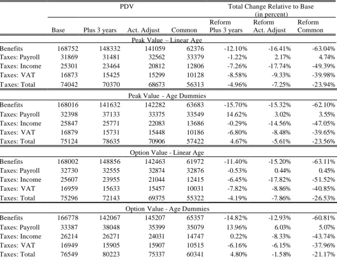
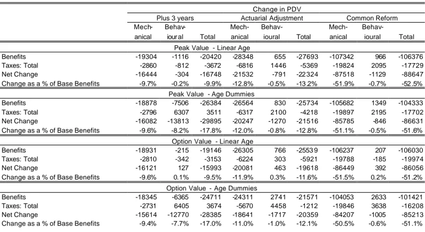
Results are better described by looking separately at each regime change, so that we can discuss the simulation strategy implemented in each specific case. An overall summary of the results is provided in Table 4 and Table 5. The former shows the total fiscal impact of the three cases R1, R2 and R3 whereas the latter decomposes these total effects into mechanical and behavioural effects. It should be noted that, although the results are presented as total effects for workers born between 1938 and 1940, the unit of analysis is really the household. To be more precise, give n our assumptions on marital status, w e describe essentially a stylized economy of married male workers (in which case we have household social security wealth) and single female workers. For brevity in this section we only comment results
obtained by making use of the option value as the incentive variable. T he full set of results can be found in the tables (Table 4 and Table 5) and corresponding figures (Figure 4 through to Figure 29). The total effects given in these tables have been obtained by aggregating the individual with weights given by the inflation factors described in Section 4 above. Because, as we shall argue, the econometric specification based on the linear term does not provide a good representation of the behaviour of Italian workers, we focus the attention on the model based on age dummies38.
R1: Age Shift (plus three years)
This reform entails a shift of the hazard by three years, while all other features of the social security system are preserved as under the baseline. The reform has a direct effect on the hazard and an indirect effect on benefits through eligibility. It should be noted that when using the linear age model the projected age profile of labor force exits does not capture well the empirical hazard (Figure1 and Figure 2) : exits are evenly distributed over ages and there is a hump around age 55 (Figure4). The empirical hazard shows instead higher variability and marked spikes at ages 55 and 60 (Figure 1). Furthermore the age distribution by age of retirement rates is essentially unaffected by the reform (Figure 4). This is because the linear term does not pick up any of the policy changes and as a result the behavioral effect is negligible.
For the model with a linear age term, the present value of benefits is reduced by 11.40% with respect to the baseline value. Because taxes are also reduced by the reform, the total net change is -9.5% (Table 4). Most of the impact of the reform is due to the mechanical effect (-9.6%).The behavioural effect, albeit very small, runs opposite to what one would expect (0.1%), because retirement probabilities are higher at younger ages after the reform and precisely at those ages losses would be higher (Table 5 and Figure 5). As for
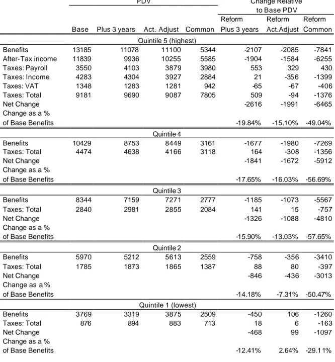
distributional effects Table 6 shows that losses are evenly spread over the population: it is the next to the highest quintile (quintile 4) which suffers most from the reform, but the loss in terms of net present value of benefits is not much higher than for the population at large.
For the model with age dummies retirement probabilities are much closer to the emprical hazard and this is clearly shown by the age distribution of labor force exits (Figure 6)39. The reform clearly affects the retirement behavior: the distribution of retirement rates is shifted toward older ages and also the spikes are observed to occur with three years delay.
38 Also, it should be noted that after age 66 there are very few workers left in the data set, so that the
estimated hazard is very volatile, we decided to set the hazard of exits (for retirement or death) equal to 0.5 after age 66 and equal to 1 at the latest age 69. The value 0.5 emerges as the estimated value at age 65, which is the last age where we have available a reasonable sample size.
39 Besides changing the eligibility rules, we increment all age dummies by three years, so that the
This implies that while a substantial fraction of the losses are suffered at ages 50 through to 57, these tend to be very high at ages 55 and 60 (the normal retirement age of women and men under the baseline). Older retirees would instead gain from the reform because of an increase in benefits at older ages.
When the econometric model allows for age dummies not only we observe a decline in benefits (-14.82% relative to the baseline), but also an increase in the overall fiscal impact (4.80%), so that the total net effect is -17.0% (Table 4 and Figures 9 and 10). This is largely die to the mechanical effect but a non negligible role is played by the behavioural effect (-7.7%) as shown in Table 5 and in Figure 8. Note that Figure 8 reports the results as a percentage of private-sector GDP: these are small (approximately -0.5% is the total effect) but one should bear in mind that social security spending is approximately 14% of total GDP in Italy. In this sense the implied saving for the budget may be non negligible. The
distributional effects of the reform are significant, with the highest quintile of social security wealth suffering a loss of approximately 20% against a 12.41% loss of the lowest quintile (Table 7). Hence, according to this model, a reform which shifts the retirement age by three years in Italy, would be effective in reducing outlays and also progressive.
R2: Actuarial adjustment
The basic idea of this Reform is to preserve the status quo in several respects, but to introduce an actuarial adjustment in order to guarantee neutrality of the system with respect to the retirement age. Before describing the results in detail it is useful to remind the reader that the baseline (pre 1993) is very far from being actuarially fair, as no actuarial penalties are envisaged for early retirement (and no bonus for late retirement).
As we argued the “linear case” is not very interesting for the Italian system, this can be easily understood by looking at Figure 11 and Figure 12, where a very smooth age profile of exit probabilities is shown, which is quite different from the observed hazard.
Focusing the attention on Figure 13 one can see that the actuarial adjustment reform has some effect on the age distribution of retirement probabilities. In fact, although their basic pattern is unchanged after the reform, exits from the labor force are lower at younger ages and higher at older ages. Coupled with the actual reduction of benefits that the reform envisages for younger retirees (Figure 16), this implies that gross benefits are reduced (-12.93%). Since also total taxes are marginally reduced (-1.58%), the net effect is -12.1% of baseline gross benefits (Table 4 and Table 5). The effect is largely due to the actual reduction in benefits, i.e. the mechanical component is prevalent (-11%), but the behavioural effect goes in the
expected direction (Table5 and Figure 15). In terms of private-sector GDP the revenue gains are of the order of 0.4 percentage points. The distributional effects are interesting both in terms of age distribution and in terms of welfare. Losses are concentrated in the age group 50
to 57 while gainers are retirees aged 58 to 69 (Figure 14). A clear ranking also emerges in terms of wealth distribution: the highest losses are suffered by the groups of the “rich” retirees (-15.1% and -16% respectively for the 5th and 4th quintiles of social security wealth, while the “poor” retirees gain from this reform (Table 7).
R3: Common Reform
The common reform is an hypothetical reform which introduces very different rules from the ones which are currently in place in Italy . On average benefits are lower: the gross
replacement rate for a fully eligible Italian worker is 80% at age 60 under the baseline, but would become 60% at age 65 under the common reform. Penalties for early retirement are non existent under the baseline, but would be substantial under R3. One further important difference is in the indexation rule: in the pre-1993 system , benefits were indexed to nominal wages, while the common reform (as well as the post 1993 regime) only indexes benefits to prices. It should be noted that, in order to identify which specific feature of the reform produced the most important changes, we kept the legislation concerning capping and eligibility to minimum benefits unchanged with respect to the baseline.
Figure 20 show the distribution of labor force exits by age when use is made of the “age dummies” model40. This reform reduces the exit rates at younger ages and shifts their distribution toward older ages. Gross benefits are muc h lower at all ages, in particular at ages between 50 and 60. Table 4 shows that, for all the reasons given above, the total impact on gross benefits is huge (-60.8%) but also taxes are lower, particularly income tax, so that the total net effect with respect to baseline benefits is -51.1% . This is almost completely explained by the mechanical effect which swamps the small gain due to delayed retirement (Table 5). As shown in Figure 22 the total effect is quite sizeable in terms of GDP: the fiscal authorities would gain approximately 1.6% of private-sector GDP.
The largest losses are suffered by workers retir ing at ages 55 and 60, which are the normal retirement ages under the baseline. In general the bulk of the fiscal saving for the government comes form the age group 50 to 60 (Figure 21). In terms of wealth distribution everyone loses from the reform, but the “median retiree” appears to lose more (3rd quintile), whereas retirees placed at the lowest quintile suffer the smallest loss (table 9).
R4: The Dini reform
40 The effect of the age dummies estimated in the hazard of exits (to retirement and to death) is slightly
modified in this simulation to take account of the fact that we have implicitly moved forward the normal retirement age. Therefore the age effect observed at age 60 should be felt at age 65 after the reform. The change is done through a smoothing procedure.
This is an actual reform enacted in 1995 by the Dini government. As described in Sections 2 and 3 above, at the steady-state, this reform would represent a radical departure from the baseline in all respects. By introducing a notionally defined contribution method of calculation of benefits it implies a potential reduction in the present value of benefits for many workers. It also introduces actuarial principles in the benefit computation formula as well as indexation to prices. The rules that this reform envisages (we stress, at the steady state) are not dissimilar from what proposed by the common reform (R3).
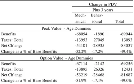
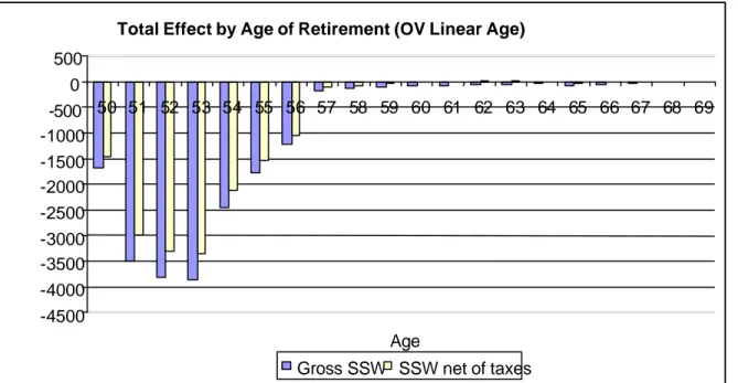
Figure 25 shows the age distribution of exit probabilities, these are all shifted to older ages both because we impose that people cannot retire before age 57 and both because incentives are such that it is optimal to postpone retirement. The reduction in gross benefits is substantial at ages 50 to 60 (Figure 28). As a results, gross benefits are reduced by 41.53% and taxes increase by 16.24% (Table 8). This is due both to a substantial mechanical effect (-31.9%) and a marked behavioural effect (-17.1%) which produce a net effect of -49% of benefits. The bulk of the losses is concentrated in the age group 50 to 56, while the older group
experiences a gain in terms of gross benefits, largely offset by an increase in taxes (Figure 26). In terms of the private-sector GDP this reform would imply a gain for the government budget of approximately 1.6%.
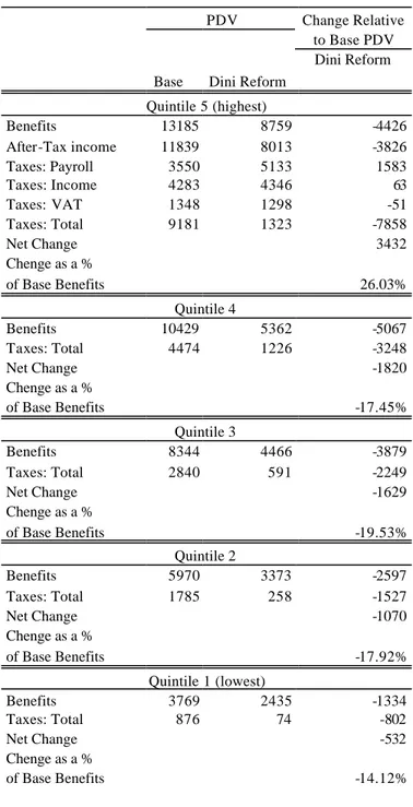
The distributional impact of the reform is somewhat perverse in our simulation, as the highest social security wealth quintile gains from the reform while all the rest of the cohort suffers a loss, particularly the “median” group (Table 10).
6.Conclusions
The reform process that many advocate for the Italian social security system has hardly been analyzed on micro data. On the other hand, the few econometric studies available do not consider the total budgetary implications of the proposed pension reforms. In this paper, we offer a novel approach to evaluating reforms which derives the entire range of fiscal implications by taking behavioral effects into account.
Our work builds on the econometric estimates in Brugiavini and Peracchi (2001), based on a longitudinal sample of private sector employees provided by the Italian Social Security Administration (INPS). A new release of these by INPS allows us to employ a richer model, also briefly described in the paper.
The simulation exercise considers three hypothetical reforms plus the actual reform
introduced in Italy in 1995 (the so-called Dini Reform). These reforms are evaluated against a baseline represented by the pre-1992 system. The hypothetical reforms range from marginal variation of the status to an “ideal” system. The first regime change (R1) is a shift of three years in all retirement ages, the second (R2) proposes an actuarial adjustment to benefits such
that early retirement is discouraged while providing incentives to delay exits. A reform common to all countries participating to the project (R3) allows us to evaluate the effects of a regime change that is quite radical in the Italian case, as it implies a sharp benefit cut, an actuarial adjustment, and a change in the indexation rules. Finally, a full application of the Dini reform (R4) changes many features of the current system. In particular, it introduces a notionally defined contribution method of benefits computation. In several dimensions, this actual reform shows similarities with the hypothetical “common reform”.
The simulations are carried out by focusing on the cohorts of workers born in the years 1938, 1939 and 1940. For these workers, we construct measures of all the variables of interested, including projected probabilities of retirement under each policy regime.
Analyzing the three hypothetical reforms against the baseline, we find that even a modest change in the effective retirement age would imply non negligible effects. If measured as a percentage of pre-reform gross benefits, losses for the workers in our cohorts are
approximately 17%. Grossing up to the population size of the cohorts considered and measuring as a percentage of the Italian output, this change is equivalent to approximately 0.5% of the GDP produced in 2001 by the private sector. The losses for the retirees represent savings for the government budget that come through reduction in benefit outlays and increases in social security contributions, income tax revenue and VAT revenue.
The actuarial adjustment reform and the common reform are particularly interesting for the Italian case. The former introduces in the baseline (pre-1993) regime an actuarial adjustment, leaving unaffected all other aspects of the social security system. This change has some effects on the age distribution of retirement rates as workers tend to delay retirement. Coupled with the actual reduction of benefits that the reform envisages for younger retirees, we obtain a net total effect of -12.1% of baseline gross benefits. In terms of GDP, the revenue gains are of the order of 0.4 percentage points. The common reform reduces the probability of exit at younger ages and shifts the distribution of retirement rates towards older ages. Gross benefits are much lower at all ages, and particularly at ages between 50 and 60. The total impact on gross benefits is huge, but due to a reduction in the total tax burden, the overall net effect is a loss to workers of 51.1% relative to the baseline case. This is almost completely explained by the mechanical effect, which swamps the small gain due to delayed retirement. The total effect is quite sizeable in the aggregate: fiscal authorities would gain approximately 1.6% of GDP.
Finally, the Dini reform of 1995 also introduces radical changes in the Italian pension system which we evaluate, in our simulations, at the steady state. The age distribution of retirement rates is shifted towards older ages both because workers cannot retire before age 57 and
because incentives are such that it is optimal to postpone retirement. The reduction in gross benefits, leading to an almost uniform distribution of benefits under the new regime, is substantial at ages 50 to 60. Overall, the net effect is a 49% benefit loss for workers in the chosen cohorts. If fully implemented in 2001, this reform would imply a gain for the government budget equal to about 1.6% of the private sector GDP.
The general conclusion is that, in Italy, there is still room for reforms which would imply non negligible saving for the government budget. Some of these reforms would also have desirable properties in terms of redistribution between generations , and between “rich” and “poor” retirees. Further research is needed to assess the effects of these reforms for a larger number of cohorts, and to analyse the distributional impact of the regime changes in several dimensions.
References
Barbi E. (2001), Aggiornamento ed analisi delle caratteristiche strutturali d ei coefficienti di
trasformazione previsti dalla legge 335/1995, in Commissione per la Garanzia dell’Informazione Statistica, Presidenza del Consiglio dei
Ministri, Completezza e Qualità delle Informazioni Statistiche Utilizzabili Per La
Valutazione della Spesa Pensionistica, Rapporto di Ricerca coordinato da F. Peracchi, Rome
Brugiavini A., (1999), Social security and retirement in Italy, in Gruber J. and D. Wise (eds.) Social
Security and Retirement around the World, The University of Chicago P ress, Chicago.
Brugiavini A. and F. Peracchi (2001), Micromodeling of retirement in Italy, Quaderni CEIS,
Università degli studi di Roma, Tor Vergata, n.147 , Rome.
Brugiavini A., F. Peracchi and D. Wise (2002), Pensions and Retirement Incentives. A Tale of three Countries: Italy, Spain and the U.S.A., forthcoming in Il Giornale degli Economisti.
Commissione per la Garanzia dell’Informazione Statistica, (2001) Presidenza del Consiglio dei Ministri, Completezza e Qualità delle Informazioni Statistiche Utilizzabili Per La
Valutazione della Spesa Pensionistica, Rapporto di Ricerca coordinato da F. Peracchi, Rome
Commissione Ministeriale per la valutazione degli effetti della legge n. 335/95 e successivi
provvedimenti, (2001), “Verifica del sistema previdenziale ai sensi della legge 335/95 e successivi provvedimenti, nell’ottica della competitività, dello sviluppo e dell’equità”, Final Report, Ministry
of Welfare.
European Commission (2000a), “Public Finances in EMU – 2000”, European Economy - Reports and
Studies, No 3.
European Commission (2000b), The contribution of public finances to growth and employment: quality
and sustainability, Communication of the Commission to the Council and the European Parliament,
COM(2000)846
European Commission (2001), ‘Public Finances in EMU – 2001’, forthcoming in European Economy
- Reports and Studies
Fornero E. e O. Castellino (2001), La Riforma del Sistema Previdenziale Italiano, Il Mulino, Studi e Ricerche, Bologna
Franco D. (2002), “Italy: A never -ending pension reform”, in M. Feldstein and H. Siebert (eds.), Social Security Pension Reform in Europe, The University of Chicago Press
Gruber, J. and D.A. Wise (1999), Social Security and Retirement around the World, The University of Chicago Press, Chicago.
Ministero del Tesoro (1999), Aggiornamento del modello di previsione del sistema pensionistico della RGS: le previsioni ’99, June.
Ministero dell’Economia (2001), Aggiornamento del modello di previsione del sistema pensionistico della RGS: le previsioni ’00, June.
OECD (1998) Maintaining Prosperity in an Ageing Society, Paris
OECD (2000b) Labour Force Statistics , 1978-1998, Part III, Paris
Peracchi F. and N. Rossi (1996), Nonostante tutto è una rifo rma, in Le Nuove Frontiere della Politica
Economica, F. Galimberti, F. Gavazzi, A. Penati and G. Tabelloni (eds.), Il Sole-24-ore,
Milan, p. 63-164.
Appendix
The Treatment of Taxes and Contributions
We have made use of four different types of taxes. These are estimated for the years between 1973 and 1996 (the period in which we observe the real labour force exit) and then projected 20 years forward.
First we use contributions (or Payroll Taxes ) paid by both the employee and the employer. The source is INPS ( www.inps.it/Doc/Professionista/aliquote/aliquote.htm) for the years 1991 to 2000. For the years between 1973 and 1990 we refer to “Relazione Generale sulla Situazione Economica del Paese” published by Ministero della Programmazione Economica e del Tesoro. T he contribution rate paid by employees increases every year, from 0.0635 of gross earnings in 1973 to 0.0889 in 1999. The rate paid by employer increases from 0.1345 to 0.2381 in 1999.
Next we use Income Taxes both for earnings and for pensions. In Italy there are several income brackets attracting different tax rates (see “Testo Unico delle Imposte sui Redditi” ). From 1974 to 1982 we could count 32 income brackets which we grouped into 9 groups in order to compare with the legislation of the 1990s. We modify also the tax rates accordingly (these range from 10% to approximately 60%). In this dataset we have included also rates to calculate the deductions for employees and pensioners. There are different deductions values for every income bracket and for every year .
The third type of taxes are Value Added Taxes which would be collected on expenditures. There are mainly four VAT tax rates which apply to different goods and services. We create a basket of goods and services with a related prices index. From this we infer an average VAT rate to be applied on expenditures . This has been changing every year: the order of magnitude is 0.09089 in 1982; 0.09521 in 1983; 0.10763 until 1993 and then decrease slightly. As in our data we only observe earnings, we calculate the total value of this tax as a percent age of earnings, taking account of the “average propensity to consume”. This is approximately 70% of income which is about 55% of earnings.