Bayesian allocation using the skew normal distribution

(1)

UNIVERSITÀ DEGLI STUDI DI ROMA

"TOR VERGATA"

FACOLTA' DI SCIENZE MATEMATICHE FISICHE E NATURALI

DOTTORATO DI RICERCA IN

MATEMATICA

CICLO DEL CORSO DI DOTTORATO

XIX

Titolo della tesi

BAYESIAN ALLOCATION USING THE SKEW NORMAL

DISTRIBUTION

Nome e Cognome del dottorando

Francesco Simone Blasi

(2)

(3)

List of Figures

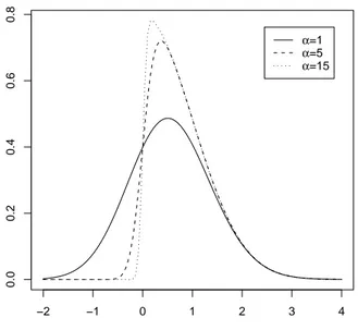
1.1 Density function SN (α) for three values of α . . . . 22

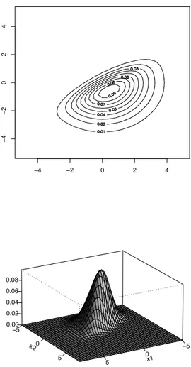
1.2 Contour plot and 3-d plot of a bivariate SN2(µ, Ω, α) with µ = (0, 0),

Ω = diag(3, 2.5) and α = (2, −3) . . . . 30

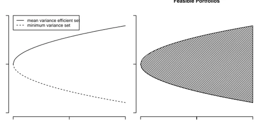
3.1 Two graphs in the space (mw, vw), where the mean is represented in the vertical axes. On the left: the minimum variance set and the efficient subset. On the right: the set of feasible portfolios. . . 43

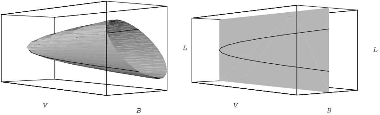
4.1 Plot of the minimum spherical variance set in the (L, V, B) space and intersection curve with the generic plane B = k . . . . 68

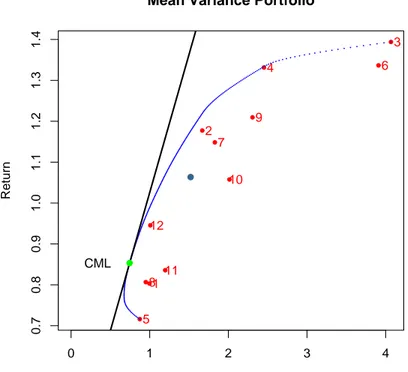
6.1 Mean variance efficient set for the portfolio of 12 strategies in the normal assumption. The tangency portfolio (0, 85%, 0, 74%) and the equally weighted portfolio (1, 06%, 2, 03%) are also represented. . . . 94

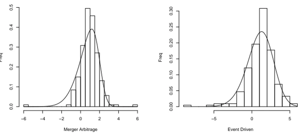
6.2 Histograms of Merger Arbitrage and Event Driven Strategies and the two

marginal densities. The curve on the left is the density of a SN (1.98, 1.65, −2.81), on the right of a SN (2.51, 2.27, −1.40) . . . . 98

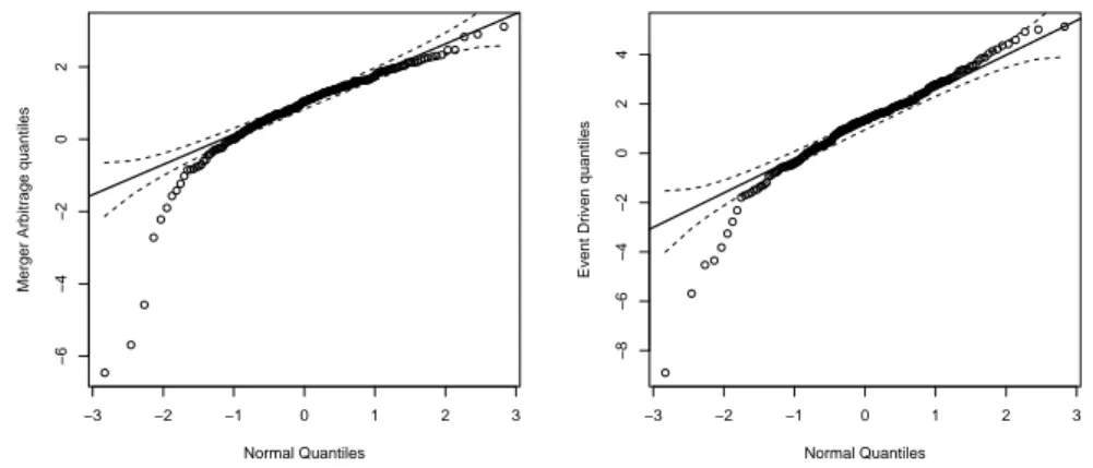
6.3 QQ-plots for the Merger Arbitrage and the Event Driven Startegies . . . 99

6.4 Plots of 30000 feasible portfolios (in grey) and of 30000 portfolios lying in the minimum spherical variance set (in black) in the (L, V = v2

w, B)-space for the portfolio of the 12 HF Strategies . . . 101

(6)

0

Introduction

Since the seminal work of Markowitz [25], portfolio theory has been improved in many directions. In order to adapt this theory to the great varieties of investment opportu-nities in modern large markets, many modifications of the mean-variance analysis have been developed.

One of the greatest limits of the theory of Markowitz consists in the assumption that all investors preferences can only be represented by the mean and the variance of returns. This assumption is coherent with the utility maximization only in two cases: either securities returns are assumed to be elliptically distributed or the investors utility func-tion is quadratic (see for instance Ingersoll [18]).

Both hypothesis are subject to two traditional criticisms. As far as the elliptical distri-butional hypothesis is concerned, many papers show the importance to include higher moments of the portfolio return in the investment process (see e.g. [30] for the stock market). In [19], it is shown that, even though hedge funds indices are often very at-tractive in mean-variance terms, this is much less the case when skewness and kurtosis are taken into account. The restriction on the class of utility functions also leads to several inconsistences.

The non-elliptical modeling of financial returns has been the subject of many papers. In our opinion, the Skew-Normal distribution of Azzalini and Dalla Valle [5], represents one of the most attractive options. This distribution has been used by Meucci in [28] for investment problems.

This choice has two main advantages: first, in opposition to many modeling propos-als, the skew-normal distribution has a coherent multivariate formulation; second, this

(7)

class maintains many useful properties that are typical of the normal distribution. Its characteristics are analyzed in details in [3], [4] and [9].

It is worth recalling that a random vector Z ∈ Rn _{follows a skew-normal distribution} with location parameter µ ∈ Rn_{, (n × n)−scale matrix Ω and shape parameter α ∈ R}n if its density has the following form:

f_Z(x) = 2ϕ_n(x; µ, Ω)Φ(αTω−1(x − µ)) (1)

where ω is the diagonal matrix ω = diag(√Ω₁₁, . . . ,√Ω_nn), √Ω_ii 6= 0 for i = 1, . . . , n, ϕn(x; µ, Ω) is the density of a Nn(µ, Ω)-random vector and Φ(x) is the cumulative distribution function of a univariate standard normal. In this case we write Z ∼

SNn(µ, Ω, α).

The main properties of the skew-normal distribution are analyzed in Chapter 1, in which the most basic facts are proved. Several modifications of this distribution have also been developed in literature. For instance, Liseo and Loperfido presented the so called ”hierarchical” skew-normal (see [23]): this distribution has been conceived in a Bayesian framework, therefore showing the great adaptability of the skew-normal class to Bayesian inference. This class can also be obtained by conditioning a multivariate normal to one of its components, with a constraint on this component. The same generation method has been applied to other elliptical distributions, in particular to the t-Student. The classes of distributions generated in this way are called, respectively, skew-elliptical and skew-t. Sahu et al. in [34] introduced a slight modification of this method for linear regression models where errors are assumed skew-t. Many interesting applications of the skew-elliptical class are exposed in the survey of Genton [14] . In this thesis, the skew-normal distribution is used to model securities returns. For the purpose of our research, it is important to focus on this modeling assumption (explicitly made in Chapter 4):

Given a vector of location parameters µ ∈ Rn_{, a vector of parameters (related to} the shape parameter α) δ ∈ Rn_{, a diagonal matrix of standard deviations ω and a} correlation matrix Ψ, we assume that the vector of returns of n risky securities is described by the following model:

R = µ + (ωδ)|X| + ω(Id − ∆2)1/2Z (2)

X ∼ N (0, 1) Z ∼ Nn(0, Ψ)

(8)

where X, Z are independent r.v.’s, ∆ = diag(δ1, . . . , δn) and Id denotes the identity matrix (see Azzalini [3] on this representation). The link between (2) and (1) is given by the following result:

Proposition. The random vector R given by (2) is skew normally distributed. More precisely R ∼ SNn(µ, Ω, α) where

Ω = ωΩω

Ω = δδT + (Id − ∆2)1/2Ψ(Id − ∆2)1/2

α = Ω−1δ

(1 − δTΩ−1δ)1/2

Note that for δ = 0 we have ∆ = 0 (the null-matrix) and therefore from (2)

R ∼ Nn(µ, ωΨω).

In the realistic example presented at the end of this thesis, we will show that for the hedge funds market, the hypothesis δ 6= 0 can be accepted (i.e. δ = 0 is rejected), validating the skew normal assumption.

We now come to the asset allocation problem which represents a considerable part of this work and has significant practical implications.

We assume that an investor selects at time t a portfolio of assets which is hold unchanged until time τ > t. A portfolio is defined as a vector

w ∈ Rn such thatXwi= 1.

By definition the portfolio return at time τ is a realization of the univariate random variable

Rw = wTR

Given two portfolios and considered their random returns R_w₁ and R_w₂, an investor is faced with the following problem:

Among the two portfolios w1 and w2, which one should be preferred?

If Rw2(·) ≥ Rw1(·) was true for each scenario then the choice would be obvious.

Nonetheless portfolio returns usually do not satisfy the previous simple dominance relation. Indeed Rw1 and Rw2 may have intersecting probability densities on ample

(9)

regions of the returns space.

The Stochastic Dominance theory (SD) mainly developed by Levy in [21], [22] and by Levy and Hanoch in [16], proposes a method to handle this problem. The final output of SD is a set of reasonable rules which should be considered as guidelines for the behavior of rational investors depending on their utility functions.

In Chapter 2, after having briefly recalled the principal aspects of SD, we develop this theory for skew-normal variables.

In short, the setup of SD is the following one: given two univariate random vari-ables R1 and R2, which in this context are often called uncertain prospects, we write

R1 º R2if R1 is preferred to R2. We denote by Uithe following sets of utility functions: U1= {u ∈ C1(R) with u0(x) ≥ 0}

and

U₂ = {u ∈ C2(R) with u0(x) ≥ 0, u00(x) ≤ 0}, then the core of SD relies in the following definition:

Definition. aaa

(1)We say that R1 stochastically dominates at first order R2 , and write R1 º1 R2, if:

E(u(R1)) − E(u(R2)) ≥ 0 (3)

for every u ∈ U1.

(2)We say that R₁ stochastically dominates at second order R₂ , and write R₁ º₂ R₂, if:

E(u(R1)) − E(u(R2)) ≥ 0 (4)

for every u ∈ U₂.

(whenever the inequalities (3) or (4) hold strictly for at least one u then we say that SD holds in strong sense).

The use of SD criteria for portfolios ranking is motivated by this important classical result:

Proposition. Given two uncertain prospects R1 ∼ N (µ1, σ1) and R2 ∼ N (µ2, σ2),

(10)

In the applications to portfolio selection and management the uncertain prospects are the returns of different portfolios. Due to the fact that the case of increasing and concave utility, describing risk-averse agents, is the most realistic one, the previous Proposition has a great worth: if two normal prospects have the same mean, the one with the smaller variance is preferable .

The following natural question arises: how can the previous Proposition be extended to skew-normal prospects whose distribution, compared to the normal law, contains a further parameter ?

Our results are summarized by the following Propositions proved in Chapter 2:

Proposition. aaa (i)Let R₁ ∼ SN (µ, σ2_{, α}

1) and R2 ∼ SN (µ, σ2, α2) be skew-normal r.v’s. Suppose

α1 ≥ α2 then R1 º1R2.

(ii)Let R1 ∼ SN (µ, σ21, α) and R2 ∼ SN (µ, σ22, α) be skew-normal r.v’s with α ≤ 0.

Suppose σ1 ≤ σ2 then R1 º2R2.

(iii)Let R1 ∼ SN (µ1, σ2, α) and R2 ∼ SN (µ2, σ2, α) be skew-normal r.v’s. Suppose

µ₁≥ µ₂ then R₁ º₁R₂.

Proposition. Let R1 ∼ SN (µ, σ12, α1) and R2 ∼ SN (µ, σ22, α2) be skew-normal r.v’s.

Suppose σ1 ≤ σ2 and σ1δ1 = σ2δ2 then R1º2 R2.

In Chapter 3 we outline the main aspects of the classical portfolio selection theory, due to Markowitz [25]. In this framework the preferences of the investor are simply codified by attitude towards mean and aversion towards variance. When market returns are normal so are portfolio returns and therefore the approach of Markowitz ranks portfolios in the same way as SD for risk-averse investors.

In the framework presented by Markowitz, the single investor fixes a level of expected portfolio return E and solves the following quadratic problem:

Minw Var(Rw) (5)

with the constraints: E(Rw) = E 1T_{w = 1}

Equivalently the agent fixes a level of risk, i.e. of standard deviation of the portfolio returns, and tries to maximize the expected return of the portfolio. The space of means and variances of portfolio returns is called the mean-variance space (MV).

(11)

Note that no assumption is made on the distributional form of the random vector R describing returns (which drives the portfolio return Rw), apart from having finite means and covariances.

Markowitz in his approach does not really take into consideration the Expected Utility (EU) maximization procedure, in the sense of Von-Neumann and Morgensten, rather he presents his theory as a self-referring one and looks forward to the practical implications. It is well known that, due to the absence of short-sale constraints1_{, problem (}₅_{) has an} explicit solution. The set of all solutions, spanned by varying the level E, is called the

minimum variance set and its generic element is given by: w∗= λ1

V−1₁ 1T_V−1₁+ λ2

V−1_m

1T_V−1_m (6)

where λi = λi(E), i = 1, 2, are such that λ1+ λ2 = 1, m = E(R) and V = Var(R)

(assumed to be not singular).

As it is evident, each portfolio given by (6) is a linear combination of only two portfolios:

w1 = V

−1₁

1T_V−1₁, w2=

V−1_m 1T_V−1_m.

Moreover it can be easily shown that any two distinct minimum variance portfolios will serve in place of w1 and w2. This result is the first example of a mutual fund separation

theorem : investors, accordingly to their selected level E of portfolio return, can form their minimum variance portfolio simply by buying (or selling) different amounts of

w1 and w2.

Let us now assume that the set of n basic market securities is enlarged by adding an extra riskless asset, which assures to the investor a fixed not random return R_f. We

shall set R₀ = R_f. Portfolios are now vectors with n + 1-components. It can be easily proven that in this case the solution to (5) is:

w∗ = λ1wf + λ2wt (7)

with λ1+ λ2 = 1, and where:

w_f = (1, 0, . . . , 0), w_t= µ

0, V−1(m − 1Rf) 1T_V−1_{(m − 1R}_f₎

¶

This is again a linear combination of only two portfolios, the portfolio w_f and the ”so called” tangency portfolio wt. Clearly, in this case, only the second one is risky. This

(12)

implies that the risky component of the investor’s portfolio is represented solely by the proportion of tangency portfolio that the investor holds.

Now suppose there are M rational agents investing in the market. Assume that they all are mean variance maximizers in the sense of (5). Furthermore assume they all have the same estimates of the means and of the covariances of the returns of the risky assets. These assumptions, together with some other ones fully listed in Chapter 3, lead to a classical result known as Capital Asset Pricing Model (CAPM), which gives the market securities expected returns and prices at equilibrium. The intuition behind the CAPM of Sharpe and Linter is based on the identification of the tangency portfolio with the market portfolio wm. Market portfolio is defined as the portfolio consisting of all securities in the market, where the weight of each security is given by its relative market value, that is, the aggregate market value of the security divided by the sum of the aggregate market values of all securities. The reasoning applied to the derivation of the CAPM can be summarized in this way: in equilibrium the aggregate demand of risky assets, which is solely represented by the tangency portfolio, is equal to the total supply of risky assets, i.e. the market portfolio. Being the tangency portfolio an efficient one so is the market portfolio at equilibrium.

The well known CAPM pricing equation, a consequence of the above identification and of the tangency condition, is then the following:

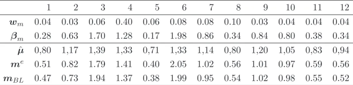
me− 1Rf = βm(mm− Rf) (8)

where mm = E(Rwm), βi,m = Cov(Ri, Rwm)/Var(Rwm) and me is the vector of

ex-pected securities returns at equilibrium.

However if the investor’s preferences are not fully captured by mean and variance of the portfolio return then the use of program (5) as decision rule for portfolio selection is questionable either from the point of view of SD or from that of EU (unless market returns are normal , or more in general elliptical). As a consequence the CAPM itself, in the form derived above, is affected by these limitations or inconsistencies.

To overcame these problems we consider in this thesis a more general approach due to Simaan [35]. More precisely, in Chapter 4 the framework considered by Simaan is explicitly worked out for the case of skew normal returns. Simaan’s methodology provides an interesting extension of the mean variance analysis since it incorporates in an elegant way investors preferences on skewness.

(13)

We remark that our interest in this extension is mainly motivated by the need of obtain-ing an equilibrium result similar to (8), which is valid in case of skew-normal returns. This step is necessary in order to produce a suitable generalization of Black Litterman portfolio selection model, which we discuss in Chapter 5 and shortly present later on. In the Simaan framework each investor controls the choice of his portfolio through the control of the location parameter wTµ and of the spherical and non-spherical

compo-nents of the variance of the portfolio return R_w, which, assuming (2) for the market returns distribution, is given by:

Var(R_w) = wTW w + µ 1 − 2 π ¶ wT[(ωδ)(ωδ)T]w. (9)

where W = (Id − ∆2₎1/2_{Ψ(Id − ∆}2₎1/2_{. In (}₉_{) the first addendum represents the}

spher-ical component of the variance while the second one the non spherspher-ical component. With relation to portfolios, we shall call the three dimensional space (location,variance,non-spherical component of the variance) the location-variance-skewness space (LVS)1 _.The name ”non spherical” component of the variance derives from the expression of the skewness of Rw:

Skew(Rw) = Skew(|X|) · (wT(ωδ))3 which is non zero, unless δ = 0.

Maximization of expected utility turns out to be equivalent, for a risk-averse investor, to the following portfolio optimization program in the (LVS) space2_:

Minw 1₂wTW w (10)

with the constraints: wT_{µ = L}

wT_{(ωδ) = B} 1T_{w = 1} for fixed L, B ∈ R.

The attractive property of (5), which is to admit an explicit solution, remains true for 1_{In his paper ,([}₃₅_{]), Simaan represents portfolios in the mean-variance-skewness space (MVS).}

There is a one-to-one correspondence between points in the (LVS) space and points in the (MVS) space (see chapter 4). When δ = 0 both spaces coincide with the mean-variance space (MV). More important, when portfolio returns are skew-normal the expected utility of a risk-verse investor behaves, as function of the parameters, much in the same way over the above two spaces.

2_{We recall that here µ identifies the locations of the returns R, while in Simaan’s paper the same}

(14)

the problem (10). We call the set of solution the minimum spherical variance set. This set includes the single portfolios with the smallest spherical part of the variance for given levels of location parameter and of non-spherical component of the variance. The generic solution can be expressed (without the riskless asset) as:

w∗ = λ₁ V−1µ 1TV−1_µ+ λ2 V−1₁ 1TV−1₁ + λ3 V−1_(ωδ) 1TV−1_(ωδ) (11)

where λ1+ λ2+ λ3 = 1 and V = Var(R).

Adding as before the riskless asset Rf to the vector of returns, the solution to (10) is given by:

w∗ = λ1wf + λ2wt+ λ3w3 (12)

where λ1+ λ2+ λ3 = 1 and where:

w_t= µ 0, V−1(µ − 1Rf) 1TV−1_{(µ − 1R}_f₎ ¶ , w₃ = µ 0, V−1(ωδ) 1TV−1_(ωδ) ¶

It is evident both in (11) and (12) that the set of solution is now a linear combination of only three portfolios. The validity of this property leads, as for the mean variance analysis, to an equilibrium result. The pricing model we obtain is fully based on Simaan results in [35], and is different from the one of Kraus and Litzenberger [20] and of Adcock [1]. Kraus and Litzenberger CAPM is based on a three moment Taylor expansion of the utility function ignoring higher moments.

This modified CAPM, obtained under the assumption (2) of skew-normality of the random vector R, relates the location parameters of the assets, µi, to the location parameters µmand µpof the portfolios wmand wp respectively. Here wmis the market portfolio defined above and wp is defined as a portfolio whose return is uncorrelated to the market portfolio return but which has its same skewness.

The CAPM equation we obtain is the following:

µe= 1Rf+ βm[µm− µp] + (γm− βm)[µp− Rf] (13)

where as before βi,m = Cov(Ri, Rwm)/Var(Rwm) and γi,m = (ωiδi)/Bm with Bm =

(wT m(ωδ))

It can be proven that the minimum spherical variance set in the (LVS) space is an elliptical paraboloid.

(15)

The result (adapted from Simaan [35]), in absence of a risk-less asset, is stated below. Let us denote Bi = (ωδ)Tai and Li = µTai where ai, i = 1, 2, 3 are the following portfolios: a1 = V −1_µ 1T_V−1_µ, a2 = V−11 1T_V−1₁ and a3= V−1(ωδ) 1T_V−1_(ωδ) (14)

and denote by B = (ωδ)T_{w and L = µ}T_{w, then the following Proposition holds:}

Proposition. If there’s no risk less asset and returns are skew normally distributed according to (2), the efficient set in the (L, V, B)−space (the LVS space) is given by:

V2 = wTV w = σ₂2+ σ_h2₃ µ B − B₂ B3− B2 ¶₂ + σ2_h₁c2₁ (15) where σ2 2 = wTa2w, σ2_h_i = wThiw, c1 = _(E(L − E2)/(E3− E2) − (B − B2)/(B3− B2) 1− E2)/(E3− E2) − (B1− B2)/(B3− B2)

and portfolios hi, i = 1, 3, are given by

h1 = (a1− a2) −B_B1− B2

3− B2(a3− a2) ; h3 = a3− a2

The final parts of Chapters 3 and 4 are devoted to the presentation of the ”so-called” mutual funds separation results. We have already presented in this introduction a particular instance of these type of theorems. More general results are available. They are directly linked to the derivation of CAPM in a general framework and for the sake of completeness are included in this thesis.

To give a rough description of general mutual funds separation results it is useful to introduce first the following definitions (Ross [32])

Definition. We shall say that,

(A) the distribution of R has the (strong) 2-funds separation property if there exist two portfolios w1, w2 such that for any portfolio wb there is a portfolio wagiven by a linear

combination of w₁ and w₂ for which it holds wT_aR º2wTbR.

(B) the distribution of R has the (strong) 3-funds separation property if there exist three portfolios w₁, w₂, w₃ such that for any portfolio w_b there is a portfolio w_a given by a linear combination of w1, w2 and w3 for which it holds

(16)

In a similar fashion k-funds separation (k ≥ 4) can be defined and discussed. The expression for the efficient portfolios given by (6) and (11) strongly suggests that the normal and skew-normal distributions have respectively the (strong) 2-funds and 3-funds separation property.

Ross in [32] gives a set of properties to be satisfied by classes of market return distri-butions in order to have a k-funds separation property:

Theorem. 1 (2-funds separation with a risk-less asset) The distribution of R has the (strong) 2-funds separation property iff

there exist a scalar r.v. Y , a vector r.v. ², a (deterministic) vector b, and two portfolios α, β such that

(a) each component of R can be written as

Ri= Rf + biY + ²i, for i = 1, . . . , n + 1

(b) E[²_i|Y ] = 0 ∀i (c) Pαi²i= 0 =

P

βi²i.

Theorem. 2 (3-funds separation with a risk-less asset) The distribution of R has the (strong) 3-funds separation property iff:

there exist two univariate r.v. Y and Q, a random vector ² , two (deterministic) vectors b, c and three portfolios α1, α2, α3 such that:

(a) each component of R can be written as

Ri = Rf + biY + ciQ + ²i for i = 1, . . . , n + 1

(b) E[²i|Y, Q] = 0 ∀i

(c) αT

i ² = 0 for i = 1, 2, 3

In the thesis we show that normal and skew normal distributions satisfy the condi-tions of Theorems 1 and 2 respectively.

We now come to the exposition of the arguments discussed in Chapter 5.

The first step of the investment process, from the investor point of view, consists in the estimation of the parameters θ contained in the distribution of the market returns

R. Within the normal assumption θ = (m, V ), whereas in the skew-normal model θ = (µ, Ω, α). The true values of these parameters being unknown, there are two

(17)

the Bayesian point of view.

By taking the first viewpoint θ is estimated directly using historical time series of re-turns: the result is a set of classical estimated parameters that we denote by ˆθ. These

values can be used as imput data to solve the portfolio problem. For instance, if the investor agrees with the Markowitz’s approach then the values ˆθ = ( ˆm, ˆV ) are used to

solve (5), with Var(Rw) = wTV w and E(Rˆ w) = wTm.ˆ

There are two main drawbacks with this approach, both well known in the literature. The first is that the selected portfolios could be not so diversified neither so intuitive. Concerning the second, the solution weights turn out to be very sensitive to changes in the estimated parameter values: when the investor updates his estimations he faces the problem of a drastic portfolio change.

We take a Bayesian point of view which helps to smooth the great sensitivity of the allocation to variations in the input data.

In the Bayesian approach parameters are considered random variables distributed ac-cording to a prior distribution, which we denote by fΘ(θ). Then it is specified a

model for the observations given the parameters, represented by the likelihood density

f_R|Θ(r|θ). From these two distributions it can be obtained the posterior density for parameters using the well known rule:

f_Θ|Rpo (θ|r) ∝ fΘ(θ)fR|Θ(r|θ) (16)

The expected utility of the portfolio return Rwis then defined conditionally on param-eters:

E(u(Rw|Θ = θ)) = Z

u(r)f_R_w_|Θ(r|θ)dr (17)

The above quantity is hence averaged over parameters by using the posterior density

f_Θ|Rpo , that is

Z

E(u(Rw|Θ))f_Θ|Rpo _w(θ|r)dθ. (18)

Then the investor can look for the optimal portfolio. However a more interesting approach is to introduce the so called predictive posterior density and take the average of the (conditional) expected utility with respect to it. Finding the optimum concludes the procedure.

(18)

However a great difficulty in handling the Bayesian approach is the fact that for many distributions the posterior density cannot be computed in closed form and numerical methods like MCMC (Monte Carlo Markov Chain) are needed.

A modified version of the classic Bayesian allocation is the Black and Litterman model (BL) appeared in [6], and discussed in detail by Black and Litterman in [7] and by He and Litterman in [17].

In the BL model security returns are assumed to be normally distributed. This model has the ability to blend together investors views and a prior on assets returns. Black and Litterman trust ˆV (sample covariance) as good estimator of V but do not trust

the sample mean ˆm. A ”modified” Bayesian approach to the estimation problem of m

is considered. They assume the following model for returns R01 _:

R0|M = m ∼ N (m; ˆV ) (19)

M ∼ N (Π, τ ˆV ) (20)

where the first requirement sets up a normal model for observed returns (given their mean), while the second chooses the prior distribution on means inside the same family.

τ is a scaling parameter, usually taken small. The vector Π is the vector of the so called

”implied returns” . It is obtained by a slight modification of the CAPM pricing equation (8) and its derivation is discussed in the chapter.

Having given a model for observations and a prior on means we could implement the previous outlined Bayesian allocation scheme. However BL model aims to incorporate into the investment process a further layer of information. This is achieved by inserting random constraints on the prior representing investors opinions on the expected values of the returns:

v − P M ∼ N (0, Ωv)

where v ∈ Rk _{is called the vector of the views, P is a k × n matrix, Ω}

v is a k × k invertible diagonal matrix and k ≤ n. It is useful introduce the r.v. V (do not confuse this vector with the covariance matrix V ), and rewrite the constraint equations in ”regression form”:

V = P M + ²

1_{More precisely R}0_{≡ R − R}

(19)

with ² ∼ N (0, Ωv). We can look to the previous relation as a model for the views (given the means), that is

V |(M = m) ∼ N (P m, Ωv)

Having a normal prior and a model for the views (again normal), we can easily obtain the posterior law of M given the views and then, integrating over M , the posterior predictive distribution of R|V . Being this distribution normal the utility is maximized by solving problem (5) and using, in place of E(Rw) and Var(Rw), the analogous moments of Rw|V which are:

mw_BL = wTm_BL

Σw_BL = wT( ˆV + ΣBL)w where:

m_BL = [(τ ˆV )−1+ PTΩ−1_v P ]−1[(τ ˆV )−1Π + PTΩ−1_v v] (21)

ΣBL = [(τ ˆV )−1+ PTΩ−1v P ]−1 (22)

Meucci in [28] and [29] extends the BL model to non normal markets relying some new ideas. This is based on the previous two stages procedure, but the Bayesian in-ference is replaced by an opinion pooling approach. Then he uses copulas to obtain the market returns distribution. This approach has the great worth to be adaptable to many non-normal markets.

On the contrary our approach preserves the Bayesian framework. This requires to make the assumption that returns are skew normal, then it uses the good properties of the skew-normal distribution under Bayesian inference , see Liseo and Loperfido [23]. In this way an analytical result for the predictive posterior of returns is obtained. More-over it can be used as ”benchmark” for further non-normal distributional assumptions, such as the skew-t.

As already explained, the BL model relies on considering the expected values of returns random variables whose density can be combined with the views vector V . In order to preserve this intuition in Chapter 6 we let the assumption (2) to be valid conditionally on locations µ. We denote by Θ1 the random vector of location parameters and we

(20)

location parameters, turn out to be a random vector as well. The market model which we assume is the following:

R|(Θ₁ = µ) ∼ SN_n(µ, Ω, α) (23)

Θ1 ∼ Nn(µe, τ Ω) (24)

where the vector µe_{is given by the pricing equation (}₁₃_{), Ω is the scale matrix of R|Θ}

1,

α its shape parameter and τ ∈ R is a small scaling factor, as previously mentioned.

Our interest in the three moment CAPM is mainly due to the need of centering the prior distribution (24) on an equilibrium vector of returns.

We prove that the model given by (23) and (24) has a skew-normal marginal for R, validating our main assumption of skew normality for assets returns.

Denoting the r.v. of expected values by M = Θ1+

q

2

π(ωδ) , the previous model can also be written in the following way:

R|(M = m) ∼ SNn(m − r 2 π(ωδ), Ω, α) (25) M ∼ Nn(me, τ Ω) (26) where me_{= µ}e₊q2 π(ωδ).

As in the BL classical model, the views are assumed to be normal :

V |(M = m) ∼ Nn(P m, Ωv), (27)

where, as before, P is a k × n matrix and Ωv is a k × k invertible diagonal matrix and

k ≤ n.

The posterior distribution of M |V is given by:

M |(V = v) ∼ N (m_BL, Σ_BL) where:

mBL = [(τ Ω)−1+ PTΩ−1v P ]−1[(τ Ω)−1me+ PTΩ−1v v] ΣBL = [(τ Ω)−1+ PTΩ−1v P ]−1

The evaluation of the posterior predictive distribution of R|V is now possible.

The result that we find combining R|M and M |V and integrating over M is the following:

R|V ∼ SNn(mBL− r

2

(21)

where

∆_BL = (Ω−1+ Σ−1_BL)−1

αT_BL = αTω−1Ω(Ω + ΣBL)−1(1 + αT∆∆BLα∆)−1/2

αT_∆ = −αTω−1dBL

and where d_BL is the diagonal matrix of standard deviations of ∆_BL and ∆_BL its correlation matrix.

After including the views in the investment process, the investor can complete the allocation process. Due to the fact that the posterior predictive distribution turns out to be skew-normal the expected utility can be maximized by the same procedure followed in chapter 4. In other terms the problem to be solved is program (10), which in this context takes the form :

Minw 1₂s2_BL (29)

with the constraints: µw_BL= E

wT_(γ BLδBL) = B 1T_{w = 1} where: µw_BL = wT(mBL− r 2 π(ωδ)) (30) s2_BL = wT(Ω + Σ_BL)w − (wT(γ_BLδ_BL))2 (31) with: δBL = q (Ω + ΣBL)αBL 1 + αT BL(Ω + ΣBL)αBL

and γBLrepresents the diagonal matrix of standard deviations of Ω+ΣBL, and Ω + ΣBL its correlation matrix.

The last part of Chapter 6 contains the main numerical example of this thesis concerning a portfolio of 12 Hedge Fund Indexes (HFR Indexes), each one corresponding to a different Hedge Funds strategy. Our assumption is that the 12 Strategies are a good representation of the Hedge Funds Market. The example covers the entire investment

(22)

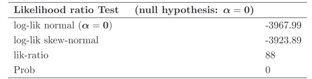
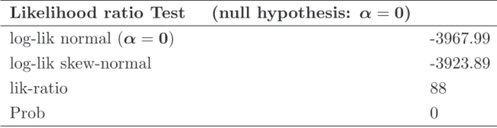
Likelihood ratio Test (null hypothesis: α = 0)

log-lik normal (α = 0) -3967.99 log-lik skew-normal -3923.89

lik-ratio 88

Prob 0

Table 1: Likelihood ratio test: the lik-ratio is the likelihood ratio test statistics and Prob the corresponding probability.

process in a skew normal market and its final output is a vector of weights that is generated conditionally on views.

The method used to validate the assumption of skew normality is a classical likeli-hood ratio test. The model with a restriction is the one with the vector α of all zeros, which implies the normality of the restricted model. The values of the test, reported in the Table, have been compared with the values from a chi-squared distribution with 12 degrees of freedom.

The results are very promising: the skew-normal assumption seems to be much more appropriate for this very dynamic market.

(23)

Nomenclature

R Random vector of returns.

w Generic portfolio, i.e. P_iw_i = 1.

Rw Univariate random variable of portfolio returns, Rw= wTR.

u Utility function.

n The number of risky assets in the market.

1 A vector whose elements are 1.

0 A vector whose elements are 0.

m The expected value of the vector of returns.

V The covariance matrix of the vector of returns.

µ The location parameter for the vector of skew-normally distributed returns. Ω The scale matrix for the vector of skew-normally distributed returns.

α The shape parameter for the vector of skew-normally distributed returns.

ϕn(·) The density of a multivariate standard normal.

Φ(·) The cumulative distribution function of a univariate standard normal.

(24)

1

The family of Skewed

Distributions

1.1 The univariate skew normal distribution

Lemma 1.1.1. If f is a density symmetric with respect to 0, if G is a one-dimensional distribution function with density G0 _{symmetric about 0, then}

φ(z) = 2f (z)G(w(z)) is a density for every odd function w(z)

Proof. Denote by Y a random variable with density f , and by X a random variable with distribution function G, independent from Y . The first step in the proof consists in proving that W = w(Y ) has a distribution function symmetric about 0. Denote by

A a Borel set of the real line and by −A its mirror set obtained by reversing the sign

of each element of A. The formula for the change of variables is

fY(y) = fX(g−1(y))|_dyd g−1(y)| (1.1)

for two random variables X and Y = g(X), then, for Z = −Y we have:

fY(t) = | − 1| · fZ(−t) = fZ(−t) (1.2)

In addition, being f symmetric, we obtain

(25)

1.1 The univariate skew normal distribution

The following equalities hold:

P{W ∈ −A}(1)= P{−W ∈ A}(2)= P{w(−Y ) ∈ A}(3)= P{w(Y ) ∈ A} (1.4)

Equality (1) is obtained by

P{W ∈ −A} = Z

−A

hW(t)dt , (1.5)

where hW(w) is the density of W and by P{W ∈ −A} = Z −A h_W(t)dt = − Z A h_W(t)dt = − Z A h−W(−t)dt = callings = −t = − Z A h−W(s)(−ds) = = Z A h−W(s)ds = P{−W ∈ A} (1.6) where we used hW(t) = h−W(−t). (1.7)

As far as equality (2) is concerned, it holds

P{−W ∈ A} = P{−w(Y ) ∈ A} = P{w(−Y ) ∈ A} (1.8)

where we used w(x) is odd.

Finally for the equality (3) we note that P{w(−Y ) ∈ A} = Z A w(t)f−Y(t)dt = Z A w(t)fY(t)dt = P{w(Y ) ∈ A} (1.9) As a result:

P{w(Y ) ∈ −A} = P{w(Y ) ∈ A} (1.10)

that implies that W = w(Y ) has a distribution function symmetric about 0.

The second step in the proof consists in noting that the random variable X − W has distribution function symmetric about 0:

P{X − W < 0} = P{X < W } = P{X > −W }

(26)

Finally we have 1

2 = P{X < W } = E{P{X < w(Y )|Y = y}} =

Z _∞ −∞ fY(y)dy Z _w(y) −∞ fX(x)dx (1.12) and 1 2 = Z _∞ −∞ G{w(y)}fY(y)dy (1.13)

which gives the desired result.

Setting f (x) = ϕ(x) and G(x) = Φ(x), the density and the distribution function of a standard normal r.v. respectively , and setting w(x) = αx with α ∈ R, we obtain the following density:

f (x) = 2ϕ(x)Φ(αx), x ∈ R (1.14)

Definition 1.1.1. A random variable Z having density (1.14) is called skew-normal (SN) with shape parameter α and denoted by

Z ∼ SN (α).

If

Y = µ + σZ,

with µ, σ ∈ R and σ > 0, then we write

Y ∼ SN (µ, σ2, α).

Its density is:

fY(y) = 2ϕ(y − µ_σ )Φ(αy − µ_σ ), y ∈ R (1.15)

The following properties for (1.14) hold: i) If α = 0 then Z ∼ N (0, 1)

ii) If Z ∼ SN (α) then −Z ∼ SN (−α)

iii) As α → ∞ then (1.14) converges point-wise to the half normal density 2ϕ(z) for

(27)

1.1 The univariate skew normal distribution −2 −1 0 1 2 3 4 0.0 0.2 0.4 0.6 0.8 α=1 α=5 α=15

Figure 1.1: Density function SN (α) for three values of α

Proposition 1.1.1. The moment generating function of X ∼ SN (µ, σ2_{, α) is:}

M (t) = E(eXt) = 2eµt+σ2t2/2· Φ(δσt) (1.16)

where

δ = √ α

1 + α2 ∈ (−1, 1)

The previous Proposition is immediate given the following result:

Lemma 1.1.2. If U ∼ N (0, 1) and a, b ∈ R then

E(Φ(a + bU )) = Φ µ a √ 1 + b2 ¶ (1.17) Proof. We have E(Φ(a + bU )) = Z _∞ −∞ ·Z ₀ −∞ 1 √ 2πe −t+(a+bu)2₂ _dt ¸ 1 √ 2πe −u2₂ _du = Z ₀ −∞ Z _∞ −∞ e−12 [u2(1+b2)+2ub(a+t)+(a+t)2]dudt (1.18)

(28)

The following known result

Z _∞ −∞ e−ax2+bxdx = r π ae b2 4a

can be applied in order to obtain the desired equality Z ₀ −∞ 1 √ 2π b2 √ 1 + b2e b2(a+t)2 2(1+b2) _e(a+t)22 dt = Z ₀ −∞ 1 √ 2π 1 √ 1 + b2e −_2(1+b2)(a+t)2 dt

which gives the result.

Proof of Proposition 1

We have for X ∼ SN (µ, σ2, α) that

Z _∞ −∞ 2√1 2π 1 σe tx_e−(x−µ)2_2σ2 "Z α(x−µ) σ −∞ 1 √ 2πe −t2 2dt # dx = Z _∞ −∞ 2√1 2π 1 σe −(x2−2x(µ+σ2t)+µ2_2σ2 "Z α(x−µ) σ −∞ 1 √ 2πe −t2 2 dt # dx = Z _∞ −∞ 2√1 2π 1 σe −(x2−2x(µ+σ2t)+(µ+σ2t)2−2µσ2t−σ4t2_2σ2 "Z α(x−µ) σ −∞ 1 √ 2πe −t2₂_dt # dx = Z _∞ −∞ 2√1 2π 1 σe µt+σ2t2₂ _e−(x−(µ+σ2t))2_2σ2 "Z α(x−µ) σ −∞ 1 √ 2πe −t2₂ _dt # dx. (1.19)

By the following change of variable

u = (x − (µ + σ2t)) σ we obtain 2eµt+σ2t22 Z _∞ −∞ 1 √ 2πe −u2₂ ·Z _ασt+αu −∞ 1 √ 2πe −t2₂_dt ¸ du

and Lemma1.1.2can be applied to obtain the desired result:

M (t) = E{eXt} = 2eµt+σ2t2/2· Φ(δσt) ¤ (1.20)

The cumulant generating function of X ∼ SN (µ, σ2, α) is the following: K(t) = log M (t) = µt +σ2t2 2 + log(2Φ(δtσ)) Thus if Z ∼ SN (α) we have: K(t) = t 2 2 + log(2Φ(δt))

(29)

1.2 The multivariate skew normal distribution and therefore µz:= E(Z) = _dtdKz(t)|t=0= (t + Φ 0_(δt) Φ(δt)δ)t=0= r 2 πδ and E(X) = µ + µ_zσ = µ + r 2 π(σδ)

The second and the third moment are given by:

Var(X) = d2 dt2K(t)|t=0= σ2− 2 π(δσ) 2 _{= σ}2_{(1 − µ}2 z) (1.21) Skew(X) = 4 (2π)3/2(4 − π)(σδ) 3 _(1.22) and furthermore γ1= 4 − π₂ µ 3 z (1 − µ2 z)3/2 , γ2 = 2(π − 3) µ 4 z (1 − µ2 z)2 where γ1, γ2 denote the standardized third and fourth-order moments.

1.2 The multivariate skew normal distribution

The following Lemma can be easily proven , it is a simple generalization of Lemma

1.1.1to the multivariate case.

Lemma 1.2.1. If f0 is a n-dimensional density function such that f0(x) = f0(−x) for

x ∈ Rn_{, G is a one-dimensional differentiable distribution function such that G}0 _{is a}

density symmetric about 0, and w is a real valued function such that w(−x) = −w(−x) for all x ∈ Rn_{, then}

f (z) = 2f0(z)G(w(z)) (1.23)

is a density function on Rn

Generalizing the univariate case, we set f0(x) = ϕn(x; 0, Ω) where Ω is a positive definite matrix, G(x) = Φ(x) and w a linear function. Then

f (x) = 2ϕn(x; 0, Ω)Φ(αTω−1x) (1.24)

is a multivariate density, where we denoted with ω the diagonal matrix of standard deviations of Ω. Allowing the presence of a location parameter µ the density becomes:

(30)

1.2 The multivariate skew normal distribution

Definition 1.2.1. A n-dimensional random variable Z having density (1.25) is called multivariate skew-normal and denoted by:

Z ∼ SNn(µ, Ω, α).

Remark: The factor ω−1 _{in (}_1.25_{) is needed in order to keep the shape parameter} unaltered when a location-scale transformation of the type Y0 _{= ξ + BY is applied to}

Y , for some positive definite diagonal matrix B and location vector ξ.

Proposition 1.2.1. The moment generating function of a random variable distributed according to (1.25) is: M (t) = 2exp(tTµ + 1 2t T_Ωt)Φ(tT_(ωδ)) _(1.26) where: δ = p Ωα 1 + αT_Ωα (1.27) and Ω = ω−1_Ωω−1

Proof. It is a simple extension of Proposition1.1.1. The first two moments are obtained from M (t):

E(Z) = µ + r 2 π(ωδ) (1.28) Var(Z) = Ω − 2 π(ωδ)(ωδ) T _(1.29)

and the multivariate index of skewness is:

γ1 = µ 4 − π 2 ¶₂Ã ₂ π(ωδ)TΩ −1 (ωδ) 1 − 2 π(ωδ)TΩ −1 (ωδ) !₃ (1.30)

The skew-normal density can be ”extended” to a more general form widely analyzed in literature (in particular see [9]). This extension is accomplished relaxing the condition on the normalization factor to be 1/2 and introducing a new parameter τ ∈ R.

Definition 1.2.2. A n-dimensional random variable Z is distributed according to the ”extended” skew normal distribution if its density is:

f_Z(x) = ϕ(x; µ, Ω)Φ(α0+ αTω−1(x − µ))/Φ(τ ) (1.31)

where α₀ = τ (1 + αT_Ωα)1/2_{. It is then denoted by}

(31)

1.2 The multivariate skew normal distribution

Remark: In the case τ = 0 also α0 = 0 and (1.31) reduces to (1.25).

An important property of the class of distributions (1.31) is the closure under affine transformations. This property will be essential in the study of portfolios returns.

Proposition 1.2.2. Given Z ∼ SNn(µ, Ω, α, τ ), ξ ∈ Rn and A a (n × d) matrix then:

ξ + AZ = Zw ∼ SNd(µw, Ωw, αw, τ ) (1.32) where: µ_w = ξ + Aµ (1.33) Ω_w = AΩAT (1.34) αw = ωwΩ −1 w HTα q 1 + αT_{(Ω − HΩ}−1 w HT)α (1.35)

where H = ω−1_ΩAT _{and ω}

w is the diagonal matrix of standard deviations of Ωw. Proof. See [4].

Another important property satisfied by the family (1.31) is the closure under marginalization. If Z ∼ SNn(µ, Ω, α, τ ) is partitioned as follows:

Z = µ Z₁ Z2 ¶ ; µ = µ µ₁ µ₂ ¶ ; Ω = µ Ω₁₁ Ω₁₂ Ω12 Ω22 ¶ ; α = µ α₁ α2 ¶ then: Z₁ ∼ SN_h(µ₁, Ω_11., α₁₍₂₎, τ ) (1.36)

where h is the dimension of Z1 and where:

α₁₍₂₎ = α1+ Ω −1 11Ω12α2 q 1 + αT 2Ω22.1α2 ; Ω22.1= Ω22− Ω21Ω−111Ω12 (1.37)

A detailed analysis of this property is presented in [4].

1.2.1 Bivariate skew normal

To better understand the properties of a skew normal distribution in this section we analyze the bivariate case. Consider the following covariances matrix:

Ω = µ ω₁2 ρω1ω2 ρω1ω2 ω22 ¶ (1.38)

(32)

1.3 Skew-t distribution

where |ρ| ≤ 1 and ωi > 0, and the shape parameter α = (α1, α2)T with αi ∈ R. The explicit expression of the bivariate skew normal density Z ∼ SN2(0, Ω, α) is, from

(1.25): fZ(z1, z2) = 2 πpω2 1ω22(1 − ρ2) e− 1 2 ω2_{1 z}2_{1 −2ρz1z2ω1ω2+ω}2_{2 z}2₂ (1−ρ2)ω2_{1 ω}₂2 _Φ µ α1 ω1z1+ α2 ω2z2 ¶ (1.39)

From (1.36) the marginal distribution of Z1 is still skew normal:

Z1∼ SN (0, ω12, α1(2)) where: α₁₍₂₎= p α1+ ρα2 1 + α2 2(1 − ρ2) (1.40)

By (1.32) the random variable Zw = wTZ with w = (w1, w2)T and Z = (Z1, Z2) ∼

SN2(0, Ω, α) is distributed according to Zw ∼ SN (µw, ωw2, αw) where:

µ_w = µ₁w₁+ µ₂w₂ ω2_w = w₁2ω2₁+ 2ρw1w2ω1ω2+ w22ω22 αw = p (α1+ α2ρ)ω1w1+ (α2+ α1ρ)ω2w2 (1 + α2λω12w21) + 2(ρα1α2λ)ω1ω2w1w2+ (1 + α21λω22w22) (1.41) and where λ = (1 − ρ2_).

Remark: As a consequence of (1.40) the distribution of Z1 is not independent from

Z2 also in the case ρ = 0. To obtain the independence it is necessary the normality of

Z2, obtained setting α2 = 0.

1.3 Skew-t distribution

In this Section we present a further distribution generated by Lemma1.2.1: the skew-t distribution. The main worth of this distribution is its ability to capture both the skewness and the thickness of the tails.

The expression of the density of a univariate t-distribution with n degree of freedom is the following: tX(x; µ, σ, n) = Γ(n+1₂ ) (πn)1/2_Γ(n/2) µ 1 +(x − µ) 2 nσ ¶_−(n+1)/2 , (1.42)

(33)

1.4 SUN

and its multivariate formulation is:

t_X(x; µ, Σ, n) = Γ( n+d 2 ) (πn)d/2_Γ(n/2) µ 1 +(x − m)TΣ−1(x − m) n ¶_−(n+d)/2 (1.43)

We denote by T1(x; n + d) the 1-dim t-cumulative distribution function with n + d

degrees of freedom. Being the t-density symmetric around the location parameter µ the assumptions of Lemma1.2.1are satisfied if one chooses: f₀ = t_Y, G(w) = T₁(w; n + d) and

w(y) = αTωy yT_Σ−1_y. In this case we obtain the following density:

fY = tY(y; µ, Σ, n) · T1 Ã αTω−1(y − m) µ n + d Qy+ n ¶_1/2 ; n + d ! (1.44)

with Qy = (y − m)TΩ−1(y − m), for any definite positive matrix Σ, location vector

µ ∈ Rd _{and shape parameter α ∈ R}d_.

Definition 1.3.1. A n-dimensional random variable Z having density (1.44) is called multivariate skew-t and we write Z ∼ Stn(µ, Ω, α, n).

Remark: In the case n → ∞ (1.44) becomes (1.25.)

We do not give here the expression of the moments of the distribution and its main properties. For a discussion of this distribution see Azzalini [3]. A modification of this distribution has been analyzed by Sahu et. al. in [34]. This new form turns out to be very useful in the regression models with skew-t errors. The main difference between the skew-t of Sahu and that one of Azzalini relies in the fact that Sahu uses the multivariate cumulative function of a t-Student as perturbation factor instead of the univariate one as in (1.44).

1.4 SUN

Several modifications of the original skew-normal density (1.31) have been developed in literature. Among these we mention the closed skew-normal (CSN) of Gonzalez-Farias

et al. [15], the hierarchical skew-normal (HSN) of Liseo and Loperfido [23] and the unified skew normal (SUN) of Azzalini Arellano [2].

(34)

1.4 SUN

In this section we briefly recall the SUN.

Consider a m + n-normal variate U = (U1, U2) :

U ∼ N_m+n(0, ˜Ω) ; ˜Ω = µ Γ ∆T ∆ Ω ¶ (1.45)

where ˜Ω is a correlation matrix. Consider now the distribution of Z = (U2|U1+γ > 0)

for some γ ∈ Rn_{. The density function of Z is computed by the formula:}

fZ(y) = fU2(y)P{U_P{U1 > −γ|U2 = y}

1 > c}

.

After simple algebra one obtains the density of Y = µ + ωZ ∈ Rn_:

fY(y) = ϕn(y; µ, Ω)Φm(γ + ∆

T_Ω−1_ω−1_{(y − µ); Γ − ∆}T_Ω−1_∆)

Φm(γ; Γ) (1.46)

Consider the vector of standard deviations ω = ω1 then:

Definition 1.4.1. A random variable Y with density given by (1.46) is called ”unified” skew normal and is denoted by Y ∼ SUNn,m(µ, γ, ω, ˜Ω)

Remark: In the case m = 1, the density given by (1.46) collapses to the density of a multivariate skew-normal (1.25).

All the properties of a SUNn,m distribution are proved in the Appendices of Azzalini-Arellano [2]. In Appendix A.1 we apply these results in order to obtain the two different types of bivariate SUNn,m, resulting from the following choice of parameters: [n = 2, m = 1] and [n = 2, m = 2].

(35)

1.4 SUN −4 −2 0 2 4 −4 −2 0 2 4 x1 −5 0 5 x2 −5 0 5 0.00 0.02 0.04 0.06 0.08

Figure 1.2: Contour plot and 3-d plot of a bivariate SN₂(µ, Ω, α) with µ = (0, 0), Ω = diag(3, 2.5) and α = (2, −3)

(36)

2

Stochastic Dominance for a

skew-normal random variable

Assume an investor selects a portfolio w of risky assets. If R is the vector of assets returns we denote by

Rw = wTR

the corresponding univariate random variable representing the portfolio return. Given two portfolio returns Rw1 and Rw2 an investor is faced with the problem:

Among the two portfolios w1 and w2, which one should be preferred?

If Rw2(·) ≥ Rw1(·) was true for each scenario then the choice would be obvious.

Nonetheless portfolio returns usually do not satisfy the previous simple dominance relation. Indeed Rw1 and Rw2 may have intersecting probability densities on ample

regions of the returns space.

The Stochastic Dominance Theory (SD), developed mainly by Levy in [21], [22] and by Levy and Hanoch in [16], represents an attractive method to solve this problem. This theory aims to find criterions to rank univariate r.v., which in this context are often called risky prospects, depending on the underlying utility functions.

Being the portfolios returns univariate r.v. they can be ranked using SD. In this way the set of all portfolios (the feasible set) breaks down into two sets: an efficient set and an inefficient set of portfolios, where a portfolio is efficient if, and only if, its re-turn is not stochastically dominated by another. Hence SD represents the base of the Portfolio Selection Theory, developed in this thesis in Chapters 3 and 4 for normal and

(37)

2.1 First and Second order Stochastic Dominance

skew-normal returns respectively.

In this Chapter after having briefly recalled the principal aspects of SD we analyze the case of normal and skew-normal prospects.

2.1 First and Second order Stochastic Dominance

We denote by U_i the following sets of functions: U1 = {u ∈ C1(R) with u0(x) ≥ 0}

U2 = {u ∈ C2(R) with u0(x) ≥ 0, u00(x) ≤ 0}

Definition 2.1.1. Consider two random variables X1 and X2, we say that X1

stochas-tically dominates at first order X2 , and we write X1 º1X2, if:

E(u(X1)) − E(u(X2)) ≥ 0

for every u ∈ U₁.

(whenever the inequality holds strictly for at least one u, then we say that SD holds in strong sense).

Lemma 2.1.1. Consider two random variables X1 and X2 which have F1(x) and F2(x)

as their cumulative distributions functions. Then if u ∈ U1:

E(u(X₁)) − E(u(X₂)) =

Z _∞

−∞

(F₂(x) − F₁(x))d(u(x)) Proof. In [16] pag. 336.

Theorem 2.1.1. Under the hypothesis of Lemma 2.1.1, then:

X1º1 X2 ⇔ F1(x) ≤ F2(x) ∀x

Proof. In [16] pag. 337.

This criterion is simply interpretable: the probability to take a value smaller than

x for X1 is not larger than the same probability for X2.

Definition 2.1.2. Consider two random variables X1 and X2, we say that X1

stochas-tically dominates at second order X2 , and we write X1º2 X2, if:

(38)

for every u ∈ U2.

(whenever the inequality holds strictly for at least one u, then we say that SD holds in strong sense).

Remark 1: We have:

X1º1 X2 ⇒ X1 º2X2

Remark 2: If X1 ºi Y and Y ºi X2 then X1 ºi X2, for i = 1, 2; this is obvious

considering that for any u ∈ Ui:

E(u(X₁)) − E(u(X₂)) = E(u(X₁)) − E(u(Y )) + E(u(Y )) − E(u(X₂)) ≥ 0

Theorem 2.1.2. Consider two random variables X₁ and X₂ which have F₁(x) and

F2(x) as their cumulative distributions functions. Then if u ∈ U2:

X₁ º₂X₂ ⇔

Z _x −∞

(F₂(t) − F₁(t))dt ≥ 0 ∀x (2.1)

Proof. In [16] pag. 338.

Given two functions g₁, g₂ defined on R. We say that g₁ intersects only once from

below g2 if g1< g2 to the left of the intersection point.

Lemma 2.1.2. Consider two random variables X1 and X2 which have F1(x) and F2(x)

as their cumulative distributions functions. If F₁(x) intersects only once from below

F2(x) in x0 , then :

E(X1) − E(X2) ≥ 0 ⇐⇒

Z _x −∞

(F2(t) − F1(t))dt ≥ 0 ∀x.

Proof. (⇒): From Lemma2.1.1: E(X1) − E(X2) = Z _∞ −∞ (F2(x) − F1(x))dx (2.2) If x ≤ x0 then _Z _x −∞ (F2(t) − F1(t))dt > 0 If x > x0: Z _x −∞ (F2(t) − F1(t))dt ≥ Z _∞ x (F1(t) − F2(t))dt > 0 (⇐): For x → ∞: Z _∞ −∞ (F2(t) − F1(t))dt ≥ 0 ⇒ E(X1) − E(X2) ≥ 0

(39)

In the next Theorem we give sufficient conditions for second order stochastic dom-inance:

Theorem 2.1.3. Consider two random variables X1 and X2 which have F1(x) and

F2(x) as their cumulative distributions functions. If F1(x) intersects only once from

below F₂(x) in x₀ then:

E(X1) − E(X2) ≥ 0 ⇐⇒ X1 º2X2

Proof. : Obvious from Theorem2.1.2and Lemma 2.1.2.

Normal random variables

Proposition 2.1.1. Consider two normal random variables X1 ∼ N (µ1, σ) and X2 ∼

N (µ₂, σ). Suppose µ₁ ≥ µ₂, then X₁º₁ X₂.

Proof. If µ1 = µ2 then X1≡ X2. If µ1> µ2 the result it’s immediate considering that

F_X₁(x) and F_X₂(x) have no intersection points and F_X₁(x) < F_X₂(x) for any x and then applying Theorem2.1.1.

Proposition 2.1.2. Consider two normal random variables X1 ∼ N (µ1, σ1) and X2 ∼

N (µ₂, σ₂). Suppose µ₁≥ µ₂ and σ₁≤ σ₂, then X₁º₂ X₂.

The proof is based on the following Lemma and on Theorem 2.1.3.

Lemma 2.1.3. Consider two normal random normal variables X₁ ∼ N (µ₁, σ₁) and

X2 ∼ N (µ2, σ2) which have F1(x) and F2(x) as their cumulative distributions functions.

Then F1(x) intersects only once from below F2(x) if and only if σ1 < σ2

Proof. The cumulative distribution function of Z ∼ N (µ, σ) can be written as:

FZ(x; µ, σ) = Z _x −∞ 1 σϕ( y − µ σ )dy = Z x−µ σ −∞ ϕ(t)dt = Φ(x − µ σ ) (2.3)

The intersection points of F1(x) and F2(x) are obtained by:

Φ(x − µ1

σ1

) = Φ(x − µ2

σ2

) (2.4)

assuming σ1 6= σ2 the previous expression implies the existence of a unique intersection

point in x∗ _{= (µ}

1σ2− µ2σ1)/(σ1− σ2). Furthermore it holds by De l’Hopital:

lim x→−∞ F1(x) F2(x) = limx→−∞Exp[− (x − µ1)2 2σ2 1 +(x − µ2)2 2σ2 2 ] = lim x→−∞Exp[− x2 2 ( 1 σ2 1 − 1 σ2 2 )] if σ1 < σ2 (σ1> σ2) then the above limit is 0 (∞). This ends the proof.

(40)

Proof. (of Proposition 2.1.2) In the case σ1 = σ2:

µ1 ≥ µ2 ⇒ X1 º1X2⇒ X1 º2 X2 (2.5)

where the first row is implied by Proposition2.1.1.

The previous Lemma implies that, if σ1 < σ2, then F1 intersects only once from below

F₂. In addition, considering the condition µ₁ ≥ µ₂ and the Theorem 2.1.3 we obtain the result.

Skew-Normal random variables

Theorem 2.1.4. : (i) Let X1∼ SN (µ, σ2, α1) and X2∼ SN (µ, σ2, α2) be skew-normal

r.v’s. Suppose α1 ≥ α2 then X1 º1 X2.

(ii) Let X1 ∼ SN (µ, σ12, α) and X2 ∼ SN (µ, σ22, α) be skew-normal r.v’s with α ≤ 0.

Suppose σ1 ≤ σ2 then X1º2 X2.

(iii) Let X₁ ∼ SN (µ₁, σ2_{, α) and X}

2∼ SN (µ2, σ2, α) be skew-normal r.v’s. Suppose

µ1≥ µ2 then X1 º1X2.

Proof:

(i): Let X ∼ SN (µ, σ2_{, α) and denote by F}

µ,σ,α(x) the corresponding distribution function. For each fixed (µ, σ) and arbitrary x we consider the function α → h(α) :=

Fµ,σ,α(x). We have: h0(α) = 2 σ Z _x −∞ ϕ(y − µ σ ) ∂ ∂αΦ(α y − µ σ )dy = 2 Z _x −∞ y − µ σ ϕ( y − µ σ )ϕ(α y − µ σ )d( y − µ σ ) = 2 Z x−µ σ −∞ tϕ(tp1 + α2_{)dt =} 2 1 + α2 Z √1+α2 σ (x−µ) −∞ tϕ(t)dt = − 2 1 + α2ϕ( √ 1 + α2 σ (x−µ))

Therefore h(α) is decreasing, Fµ,σ,α1(x) ≤ Fµ,σ,α2(x) for all x, and the result follows by

Theorem2.1.1.

(ii): For each fixed (µ, α) and arbitrary z we consider the function σ → l(σ) := R_z −∞Fµ,σ,α(x)dx. We have: l0(σ) = Z _z −∞ ∂ ∂σ[ Z _x −∞ 2 σϕ( y − µ σ )Φ(α y − µ σ )dy]dx = 2 Z _z −∞ ∂ ∂σ[ Z x−µ σ −∞ ϕ(t)Φ(αt)dt]dx = −2 Z _z −∞ x − µ σ2 ϕ( x − µ σ )Φ(α x − µ σ )dx = −2 Z z−µ σ −∞ tϕ(t)Φ(αt)dt