Reconstruction of the post-glacial volcanic activity in Iceland through paleomagnetic survey and remote sensing

Scuola

R

ECONSTRUCTION

OF THE

through Paleomagne

PhD student: dr. Annamaria PINTON

Supervisors: prof. Guido GIORDANO

dr. Fabio SPERANZA

Coordinators: prof. Claudio FACCENNA (

prof. Sveva CORRADO (

Dipartimento di Scienze

cuola Dottorale in Geologia dell’Ambiente e delle Risorse

-- SDiGAR --

sezione Geologia delle Risorse

XXVII ciclo dottorale

P

H

D

D

ISSERTATION

OF THE

P

OST

-G

LACIAL

V

OLCANIC

A

CTIVITY

aleomagnetic survey and Remote S

PINTON

__________________________________

prof. Guido GIORDANO

__________________________________

dr. Fabio SPERANZA

_{_________________________________}

rof. Claudio FACCENNA (SDiGAR)

_____________________

prof. Sveva CORRADO (Sezione “Risorse”)

__________________________________

isorse

CTIVITY

IN

I

CELAND

Sensing

__________________________________

__________________________________

________________________________

__________________________________

__________________________________

Reviewers:

dott. Elena ZANELLA

prof. Michael ORT

Academic board members:

prof. G. Diego GATTA

dott. Luca ALDEGA

dott. Roberto SULPIZIO

These years of PhD research have been full of extraordinary experiences. Travelling all around the world, discovering new theories/worlds/cultures/methods, “arguing” with samples and data, facing new possibilities, ... growing-up with my own work... Amazing!

Nothing would have been possible without my supervisors, who gave me the possibility to reach this moment. Prof. Guido Giordano was always ready to raise my spirit and enthusiasm high, suggesting new ideas, guiding my work, supporting me even in the scientifically harder moments. Dr. Fabio Speranza has been a true cornerstone throughout all these years: its experience, knowledge on paleomagnetism, its great precision and reliability have been fundamental in reassuring me when needed.

An important contribution came from dr. Rosamaria Salvatori (CNR IIA, Montelibretti, Roma), dr. Paola Cianfarra and prof. Francesco Salvini (Roma Tre University), whose advice, help, support and ideas have been essential to develop such a good and innovative approach for applying the proximal and remote sensing to Icelandic basalts. Also, their presence during the 2012 survey has been precious, for not collapsing and giving up on exhaustion. I am also grateful to the referees and the academic board members who deeply improved this thesis with encouraging advises.

The initial shock of facing Icelandic language was easily overcome thanks to the precious help of prof. Thorvaldur Thordarson (University of Iceland), who guided me through both the tricky Icelandic basalts and the written (and oral) culture, which resulted in an unconditional love for this amazing country. Also, dr. Ingibjörg Kaldal (Iceland Geosurvey) help in retrieving geological maps has been essential for dealing with Thjorsa areas.

I cannot forget the precious and unselfish help of Luca and Guðbjorn during the field surveys: despite the never-ending drilling sessions, the cold/wind/rain, the soaked feet in the icy river, they continued to support my requests without objections. Thanks also to Guðbjorn’s family for its kind hospitality.

Precious suggestions came from Anita Di Chiara, Javier Pavon-Carrasco and Catalina Hernandez Moreno about “paleomagnetic” issues, as well as from the geomorphology laboratory of Roma Tre University and from Alessandro Vona, with their useful tips on using Matlab. Thanks to Arnaldo Angelo De Benedetti: we will always have the perfect song and the perfect word for any moment!

Infine, proseguo i miei ringraziamenti nella mia amata lingua madre, l’italiano, per includere e rendere partecipi tutte le persone che mi hanno supportata sin da quando ho deciso di studiare geologia. Grazie di cuore, mamma e papà, sempre pronti a guidare per 700 km per essere più vicini a me, pronti a sostenermi, aiutarmi ed incoraggiarmi, nonostante tutti i pensieri che vi preoccupano. Grazie a mio fratello, Florinda e Gioele: siete sempre nel mio cuore e vi ringrazio per l’appoggio incondizionato a tutte le mie “grandiose” idee ed iniziative, anche quelle più strampalate. Grazie a mia sorella, Marco, Michele ed Elisa: mi siete di grandissimo incoraggiamento, con il vostro entusiasmo nel viaggiare, fare, conoscere ed esplorare! Grazie a tutta la famiglia Bussinello, che mi ha ospitato nella loro quotidianità facendomi sentire a mio agio, proprio come in una seconda casa. Grazie alle mie amiche di sempre: siamo vicine anche quando siamo lontane. Grazie a tutti coloro che non ho nominato espressamente, ma che sanno di essere nel mio cuore.

In ultimo, Harry. Il mio amore grande. Mi incoraggi ad andare avanti, a non avere paura, a mettermi in gioco anche se tutto questo potrebbe portarci lontano l’uno dall’altro: i nostri cuori rimarranno avvinghiati in qualsiasi caso. Questa tesi è dedicata anche e soprattutto a te.

Niente di grande fu mai compiuto senza entusiasmo.

Nothing great was ever achieved without enthusiasm.

land of fire and ice, is a volcanologically fascinating territory that

covers an area of about 103’000 km

_{. The 22% of its surface}

(~23’000 km

_{) is covered by Holocene volcanic deposits, mainly basaltic or basaltic-andesitic in}

composition. Such a high volcanic production is explained by the fact that Iceland lies at the

intersection between the Mid-Atlantic ridge and a mantle plume localised in the central-eastern

part of the island. The region was entirely covered by a thick ice cap that started to melt between

10200 years BP and 9000 years BP, the last marking the end of the glacial period (

).

Because of the glacial retreat and the subsequent decrease of the overlying mass, volcanic eruptions

in Iceland suddenly increased in volume and frequency during the post-glacial period (

). Presently, the number of volcanoes and eruptive fissures present in Iceland is so

huge, that they have been subdivided and organized in 30 volcanic systems (

), 28 of which, active during Holocene epoch. Sixteen of these volcanic systems were active

after the settlement of Iceland (dated 871 AD) in historical times, erupting nearly 40 km

_{of lavas}

(

). The other twelve systems erupted about 200 km

of lavas prior to 871 AD, mainly

from shield volcanoes and eruptive fissures (

).

A complete list of the most important (> 1 km

_{of volume) Holocene basaltic eruptions occurred}

in Iceland has only recently been compiled by

(

). All these eruptions, although effusive,

had a very strong in impact on climate because of the dangerous SO

emissions into the atmosphere:

the famous Laki eruption in 1783-84 AD caused severe famine and haze all over Europe (e.g.

), as other big effusive

eruptions did, both in Iceland and all over the world (e.g.

). Therefore, the assessment

of their frequency in time is, of course, very important.

In general, a detailed chronostratigraphy of the eruptive events exists only for historical

eruptions: those systems have mostly been studied and described, so that we have a deep knowledge

on these events and their distribution. On the other hand, the majority of the pre-historical events

(refer to section II). As a matter of fact, the previously mentioned list of basaltic events (compiled by

Hjartarson in

) includes areas, ages and volumes estimates that mostly come from

unpublished works and personal communications to the author and it is not possible to retrieve a

detailed geological map for the majority of the biggest events.

The difficulty in studying those volcanic events lies in different aspects. Firstly, a high

uncertainty exists on identifying lavas distributions because of the high compositional similarity

between basaltic lavas and, yet, their high internal petrographic variability within same event . This

results in a difficult correlation of distant deposits and on the subsequent difficulty in retrieving

precise volume calculations. Furthermore, it is difficult to obtain a date for pre-historical events

because of the methodological limitations in the application of the radiometric absolute dating

methods on these volcanic rocks. For example, the low K content and the lack of suitable

phenocrysts in these recent basaltic lavas makes it impossible to apply the

_Ar/

_{Ar dating.}

Seemingly, the

_{C dating method relies on the presence of paleosoils and vegetation remains, which}

are quite rare at these latitudes. This means that only scattered spots of hardly correlable lavas have

an absolute age constrain, in areas where the relative chronostratigraphy of events is already so

tricky.

In Iceland, the tephrochronology proved to be the most useful dating method, at present. It

applies to the widespread silicic tephra layers erupted from several well-known eruptions that

dispersed light volcanic material (pumice and ash) all-over Iceland. Different from

contemporaneous basalts, these Holocene felsic tephras can be dated because of their high contents

of K and, as they are preserved between undated basaltic lavas, they can provide an age constrain

and a relative date to the basaltic events.

Again, since it is not always possible to correlate distant basaltic deposits and, at most localities,

silicic tephra are not preserved between basaltic lavas (particularly in the inner areas where the

weathering caused, for example, by intense precipitations, snow melting or wind is severe), the

complete reconstruction of the chronostratigraphy of huge basaltic events is not always possible

and still considerably incomplete.

This PhD research project aimed at applying other techniques for solving those problems of

absolute datings of Holocene basaltic lavas and their areal correlation. In particular, I used the

paleomagnetic method as a correlation and dating tool for deepening the knowledge of the most

important Holocene basaltic lavas in Iceland, in terms of age and distribution. This, by collecting

samples from multiple lava outcrops and, then, by studying and comparing their registered

paleomagnetic direction (refer to section I). Also, a technique that integrates proximal and remote

sensing has been developed on a testing area: rock samples and in-situ reflectances were collected

and analysed, integrating the acquired information with Landsat 8 satellite images (refer to section

III). The application of this method to wider areas opens-up a possible future application of the

remote/proximal sensing) can be successfully applied and integrated with the available knowledge

on the studied volcanic systems for further deepen the understanding of the chronostratigraphy of

Icelandic post-glacial (Holocene) volcanic areas. Indeed, they could result in a great help for better

constraining the absolute age of deposits, as well as their distribution.

The thesis is subdivided in three sections, each one self-sustained and dealing with a different

subject. Section I “Paleomagnetism as a Correlation and Dating Tool: potential of the method at high latitudes

(Iceland)” strictly refers to the paleomagnetic methodology applied in this project, which has been

carefully analysed, verified and tested on well-known historical lavas. The paleomagnetic sampling

and measurement methods have been described (chapter 2), as well as the correlation and dating

process, which have been explained in detail in chapter 3. Also, an application of the method on

poorly known basaltic lavas has been developed (chapter 4). A general discussion (chapter 5)

concludes the first section, presenting a general conclusion of the first applications of the method

on real cases and summarizing how the paleomagnetic method will be applied in the subsequently

analysed Icelandic lavas.

Section II “Post-glacial Volcanic Activity in Iceland: a review of the main shield volcano and fissure

eruptions” applies the paleomagnetic method described in Section I to important basaltic lavas

situated in four Icelandic areas (chapters 2, 3, 4, 5). Collected paleomagnetic data are analysed and

interpreted for retrieving correlation information and an absolute age for studied lavas, which are

currently scarcely known. The subsequently drawn general conclusions (chapter 6) give a new

insight on the chronostratigraphy of Icelandic post-glacial volcanic activity, opening up new

possibilities for further improve the knowledge on the area.

In Section III “Proximal and Remote Sensing as integrated tools for studying lava deposits distribution: an

example from Iceland”, an integrated methodology is introduced and developed for applying both

proximal (chapter 2) and remote sensing (chapter 3) techniques to satellite images. Their integration

(chapter 4) helped in producing a new map with a classification of different spectral units that could

correspond to different lava units. This is still a preliminary study, but it shows how this

methodology could allow a further help in the correlation of lava units, in future. For example, the

produced classification map could support the paleomagnetic survey by suggesting useful areas

where collecting samples.

Further details follow on the calculation of the error relative to the declination in the

paleomagnetic dating process (Appendix I), the data relative to the used demagnetization processes

(Appendix II) and the measurements sites and laboratory samples photos (Appendix III).

References:

ANGELL,J.K.,&KORSHOVER,J.(1985).SURFACE TEMPERATURE CHANGES FOLLOWING THE SIX MAJOR VOLCANIC EPISODES BETWEEN 1780-1980.JOURNAL OF CLIMATE AND APPLIED METEOROLOGY,24,937–951.

CHENET,A.,FLUTEAU,F.,&COURTILLOT,V.(2005).MODELLING MASSIVE SULPHATE AEROSOL POLLUTION, FOLLOWING THE LARGE 1783LAKI BASALTIC ERUPTION.EARTH AND PLANETARY SCIENCE LETTERS,236(3-4),721–731. DOI:10.1016/J.EPSL.2005.04.046

DEVINE,J.,SIGURDSSON,H.,DAVIS,A.N.,&SELF,S.(1984).ESTIMATES OF SULFUR AND CHLORINE YIELD TO THE ATMOSPHERE FROM VOLCANIC ERUPTIONS AND POTENTIAL CLIMATIC EFFECTS.JOURNAL OF GEOPHYSICAL RESEARCH,89(B7),6309–6325.RETRIEVED FROM

HTTP://ONLINELIBRARY.WILEY.COM/DOI/10.1029/JB089IB07P06309/FULL

GRAINGER,R.,&HIGHWOOD,E.J.(2003).CHANGES IN STRATOSPHERIC COMPOSITION, CHEMISTRY, RADIATION AND CLIMATE CAUSED BY VOLCANIC ERUPTIONS.

IN C.OPPENHEIMER,D.PYLE,&J.BARCLAY (EDS.),VOLCANIC DEGASSING (PP.329–347).GEOLOGICAL SOCIETY OF LONDON,SPECIAL PUBLICATIONS (213). RETRIEVED FROM HTTP://SP.LYELLCOLLECTION.ORG/CONTENT/213/1/329.SHORT

GRATTAN,J.P.,DURAND,M.,&TAYLOR,S.N.(2003).ILLNESS AND ELEVATED HUMAN MORTALITY IN EUROPE COINCIDENT WITH THE LAKI FISSURE ERUPTION. IN C.OPPENHEIMER,D.M.PYLE,&J.BARCLAY (EDS.),VOLCANIC DEGASSING (PP.401–414).GEOLOGICAL SOCIETY OF LONDON,SPECIAL PUBLICATIONS (213).

GUDMUNDSSON,H.J.(1997).A REVIEW OF THE HOLOCENE ENVIRONMENTAL HISTORY OF ICELAND.QUATERNARY SCIENCE REVIEWS,16,81–92.

HALLDORSSON,S.,OSKARSSON,N.,GRÖNVOLD,K.,SIGURDSSON,G.,SVERRISDOTTIR,G.,&STEINTHORSSON,S.(2008).ISOTOPIC-HETEROGENEITY OF THE

THJORSA LAVA—IMPLICATIONS FOR MANTLE SOURCES AND CRUSTAL PROCESSES WITHIN THE EASTERN RIFT ZONE,ICELAND.CHEMICAL GEOLOGY,255,305–316.

DOI:10.1016/J.CHEMGEO.2008.06.050

HIGHWOOD,E.J.,&STEVENSON,D.S.(2003).ATMOSPHERIC IMPACT OF THE 1783-1784LAKI ERUPTION:PART IICLIMATIC EFFECT OF SULPHATE AEROSOL. ATMOSPHERIC CHEMISTRY AND PHYSICS DISCUSSIONS,3,1599–1629.

HJARTARSON,Á.(1994).ENVIRONMENTAL CHANGES IN ICELAND FOLLOWING THE GREAT THJORSA LAVA ERUPTION 780014C YEARS B.P.IN J.STOTTER &F. WILHELM (EDS.),ENVIRONMENTAL CHANGE IN ICELAND (PP.147–155).MÜNCHENER GEOGRAPHISCHE ABHANDLUNGEN,REIHE B.

HJARTARSON,Á.(2003).POSTGLACIAL LAVA PRODUCTION IN ICELAND.IN:ÁRNI HJARTARSON,2003.THE SKAGAFJÖRÐUR UNCONFORMITY,NORTH ICELAND, AND ITS GEOLOGICAL HISTORY.GEOLOGICAL MUSEUM,UNIVERSITY OF COPENHAGEN.PHDTHESIS,248PP.,95–108.

MACLENNAN,J.,JULL,M.,MCKENZIE,D.,SLATER,L.,&GRÖNVOLD,K.(2002).THE LINK BETWEEN VOLCANISM AND DEGLACIATION IN ICELAND.GEOCHEMISTRY, GEOPHYSICS,GEOSYSTEMS,3(11),1–25. DOI:10.1029/2001GC000282

PALAIS,J.M.,&SIGURDSSON,H.(1989).PETROLOGIC EVIDENCE OF VOLATILE EMISSIONS FROM MAJOR HISTORIC AND PRE-HISTORIC VOLCANIC ERUPTIONS.AGU MONOGRAPH,52,31–35.

RAMPINO,M.R.(2002).SUPERERUPTIONS AS A THREAT TO CIVILIZATIONS ON EARTH-LIKE PLANETS.ICARUS,156,562–569. DOI:10.1006/ICAR.2001.6808 SADLER,J.P.,&GRATTAN,J.P.(1999).VOLCANOES AS AGENTS OF PAST ENVIRONMENTAL CHANGE.GLOBAL AND PLANETARY CHANGE,21,181–196. SANTACROCE,R.(2009).VULCANI ED ESTINZIONI DI MASSA.ATTI DELLA SOCIETÀ TOSCANA DI SCIENZE NATURALI,MEMORIE,114(A),19–43.

SELF,S.,WIDDOWSON,M.,THORDARSON,T.,&JAY,A.E.(2006).VOLATILE FLUXES DURING FLOOD BASALT ERUPTIONS AND POTENTIAL EFFECTS ON THE GLOBAL ENVIRONMENT:ADECCAN PERSPECTIVE.EARTH AND PLANETARY SCIENCE LETTERS,248,518–532. DOI:10.1016/J.EPSL.2006.05.041

SIGMUNDSSON,F.(1991).POST-GLACIAL REBOUND AND ASTHENOSPHERE VISCOSITY IN ICELAND.GEOPHYSICAL RESEARCH LETTERS,18(6),1131–1134.

DOI:10.1029/91GL01342

SLATER,L.,JULL,M.,MCKENZIE,D.,&GRONVO,K.(1998).DEGLACIATION EFFECTS ON MANTLE MELTING UNDER ICELAND _{: RESULTS FROM THE NORTHERN}

VOLCANIC ZONE.EARTH AND PLANETARY SCIENCE LETTERS,164,151–164.

STEVENSON,D.S.,JOHNSON,C.E.,HIGHWOOD,E.J.,GAUCI,V.,COLLINS,W.J.,&DERWENT,R.G.(2003).ATMOSPHERIC IMPACT OF THE 1783–1784LAKI ERUPTION _{:PART ICHEMISTRY MODELLING.ATMOSPHERIC CHEMISTRY AND PHYSICS DISCUSSIONS,3,487–507.}

STOTHERS,R.B.(1998).FAR REACH OF THE TENTH CENTURY ELDGJA ERUPTION,ICELAND.CLIMATIC CHANGE,39(4),715–726.

TEXTOR,C.,SACHS,P.M.,GRAF,H.-F.,&HANSTEEN,T.H.(2003).THE 12900 YEARS BPLAACHER SEE ERUPTION: ESTIMATION OF VOLATILE YIELDS AND SIMULATION OF THEIR FATE IN THE PLUME.IN C.OPPENHEIMER,D.M.PYLE,&J.BARCLAY (EDS.),VOLCANIC DEGASSING (PP.307–328).GEOLOGICAL SOCIETY OF

LONDON,SPECIAL PUBLICATIONS (213).

THORDARSON,T.,&LARSEN,G.(2007).VOLCANISM IN ICELAND IN HISTORICAL TIME:VOLCANO TYPES, ERUPTION STYLES AND ERUPTIVE HISTORY.JOURNAL OF GEODYNAMICS,43,118–152. DOI:10.1016/J.JOG.2006.09.005

THORDARSON,T.,&SELF,S.(2003).SULPHUR RELEASE FROM FLOOD LAVA ERUPTIONS IN THE VEIDIVÖTN,GRÍMSVÖTN AND KATLA VOLCANIC SYSTEMS, ICELAND.GEOLOGICAL SOCIETY,….RETRIEVED FROM HTTP://SP.LYELLCOLLECTION.ORG/CONTENT/213/1/103.SHORT

WALLACE,P.,&CARMICHAEL,I.S.E.(1992).SULFUR IN BASALTIC MAGMAS.GEOCHIMICA ET COSMOCHIMICA ACTA,56(5),1863–1874. WIGNALL,P.B.(2001).LARGE IGNEOUS PROVINCES AND MASS EXTINCTIONS.EARTH SCIENCE REVIEWS,53,1–33.

Section I - Paleomagnetism as a Correlation and Dating Tool: potential of the method

at high latitudes (Iceland)

1. PALEOMAGNETISMASACORRELATIONANDDATINGTOOL:ANINTRODUCTION ... 5

2. PALEOMAGNETICSAMPLINGANDMEASUREMENTMETHODS ... 9

2.1 Methods ... 10

2.2 Data Analysis and in-situ Observations ... 14

2.3 Discussions ... 22

3. THECORRELATIONANDDATINGMETHOD:CONSIDERATIONSANDTESTINGOFPSVREFERENCECURVES... 25

3.1 Reference PSV curves and models considerations... 27

3.2 The Archaeo_dating tool application ... 32

3.3 Testing the methodology on the Laki and Eldgjà eruptive events ... 34

3.4 Discussions ... 39

4. APPLICATION OFTHEPALEOMAGNETICMETHODTO HIGH-LATITUDESITES:REYKJANESPENINSULAERUPTIVE EVENTS ... 43

4.1 Reykjanes data analysis ... 46

4.2 Discussions ... 48

5. GENERALDISCUSSIONSANDCONCLUSIONS ... 51

6. REFERENCES ... 57

6.1 Reference List ... 57

6.2 List of Tables and Figures ... 59

Section II - Post-Glacial Volcanic Activity in Iceland: a review of the main

shield-volcano and fissure eruptions

1.1 Methods ... 69

2. BARÐARDALURLAVASFORMATION ... 71

2.1 Geological Setting ... 71 2.2 Data Analysis ... 73 2.3 Interpretation ... 75 3. LAXARDALURLAVAS ... 77 3.1 Geological Setting ... 77 3.2 Data Analysis ... 80 3.3 Interpretation ... 82 4. THEISTAREYKJRLAVAS ... 84 4.1 Geological Setting ... 84

4.3 Interpretation ... 87

5. TUGNAÀANDTHJORSALAVAS ... 89

5.1 Geological Setting ... 89

5.2 Tugnàa Lavas Data Analysis ... 96

5.3 Thjorsa and Older Lavas Data Analysis ... 101

5.4 Interpretation ... 103

6. GENERALDISCUSSIONANDCONCLUSIONS ... 108

7. REFERENCES ... 111

7.1 Reference List ... 111

7.2 Lists of Tables and Figures ... 112

Section III - Proximal and Remote Sensing as integrated tools for studying lava

deposits distribution: an example from Iceland

1.1 Geological Setting ... 121

2. PROXIMALSENSING ... 125

2.1 Data Acquisition ... 125

2.2 Data Processing ... 129

3. REMOTESENSING ... 131

3.1 Image Processing Techniques ... 134

3.2 Image Analysis and Interpretation of Results ... 137

4. DISCUSSIONSANDCONCLUSION ... 145

5. REFERENCES ... 147

5.1 Reference List ... 147

5.2 Lists of Tables and Figures ... 148

Appendix I

Appendix II

Appendix III

I.

Paleomagnetism as a Correlation and Dating Tool:

potential of the method at high latitudes (Iceland)

1. PALEOMAGNETISM AS A CORRELATION AND DATING TOOL: AN INTRODUCTION ... 5

2. PALEOMAGNETIC SAMPLING AND MEASUREMENT METHODS ... 9

2.1 Methods ... 10

2.2 Data Analysis and in-situ Observations ... 14

2.3 Discussions ... 22

3. THE CORRELATION AND DATING METHOD: CONSIDERATIONS AND TESTING OF PSV REFERENCE CURVES... 25

3.1 Reference PSV curves and models considerations ... 27

3.2 The Archaeo_dating tool application ... 32

3.3 Testing the methodology on the Laki and Eldgjà eruptive events ... 34

3.4 Discussions ... 39

4. APPLICATION OF THE PALEOMAGNETIC METHOD TO HIGH-LATITUDE SITES:REYKJANES PENINSULA ERUPTIVE EVENTS . 43 4.1 Reykjanes data analysis ... 46

4.2 Discussions ... 48

5. GENERAL DISCUSSIONS AND CONCLUSIONS ... 51

6. REFERENCES ... 57

6.1 Reference List ... 57

1.

Paleomagnetism as a Correlation and Dating Tool:

an introduction

nderstanding the stratigraphic sequences of widespread basaltic eruptive events has always represented a highly intriguing challenge for volcanologists, especially when little geochronological dating is available or when the subtle variability of rock geochemistry does not come to assistance. This is particularly true for the Icelandic post-glacial volcanic sequence, which rests on the Mid-Atlantic ridge that

crosses Iceland and intersects a hot-spot in the central-eastern part of the island(Thordarson & Larsen, 2007).

Here a total of nearly 240 km3 _{of erupted material mainly concentrates in a relatively narrow corridor (about}

50 km wide) in the central part of Iceland and on the Reykjanes peninsula. To constrain the chronostratigraphy of all these events, the absolute age determination through isotopic dating would be advisable, but both Ar/Ar and K/Ar methods are of difficult application in such K-poor volcanic rocks.

Similarly, 14_{C datings of soil layers interposed in volcanic formations are highly scattered and do not reach the}

inner areas of Iceland, as soils and vegetation develop slowly at these latitudes and scarcely on Icelandic highlands. This makes it hard to have a complete understanding of the events sequence through time.

A remarkable support comes from the currently well established tephrochronology studies, which can

recognize all the main silicic tephra layers associated to known-age eruptions (e.g. Dugmore et al., 1995;

Haflidason et al., 2000; Larsen & Thorarinsson, 1977)that are interposed with unknown basaltic events. As both tephras and soils are not evenly preserved and distributed, we can take this scattered information to reconstruct a framework for the chronology of the basaltic events, but it is important to underline that this framework can only provide relative ages and that there are wide areas where those information are not available so that still doubts remain about datings and correlations.

In these chapters, I evaluate the possibility to take advantage of the paleomagnetic information registered by volcanic rocks during their emplacement for retrieving dating and correlation information. The basis of this method lies in the fact that erupted magmas, while cooling, record the direction of the magnetic field acting during their emplacement. Lavas emplaced at the same time, will register a similar paleomagnetic direction, thus providing a key for correlating even distant outcrops.

Furthermore, knowing how the magnetic field continuously changed through time by studying sedimentary sequences, volcanic rocks and archaeological artefacts, it has been possible to reconstruct reference curves, called PaleoSecular Variation (PSV) curves of the geomagnetic field, that describe these variations. The age of emplacement of studied lavas can be determined by comparing the direction of the

paleomagnetic field registered by the lavas with those of the PSV reference curves. Since early works on

paleomagnetic dating of volcanic rocks at Etna in 1925 (Chevallier, 1925), this method has improved and is more

and more frequently applied (e.g. Carlut et al., 2000; Hagstrum & Champion, 1994; Lanza et al., 2005; Lanza & Zanella,

2006; Rolph et al., 1987; Rutten & Wensink, 1960; Speranza et al., 2008; Tanguy et al., 2003; Thompson & Turner, 1985; Vezzoli et al., 2009; etc) in order to find the emplacement age of volcanic products or to use their registered direction as a correlation tool.

This project aims at evaluating the potential of the method at higher latitudes, and Iceland has been identified as a perfect testing area, as absolute dating and overall distribution of Holocene basaltic lavas are still largely missing or not clear. This work will start with explaining the paleomagnetic sampling and measurements methods applied in the studied Icelandic area. Considerations of the reliability of obtained data and of the possibility to deduce the correlation of lavas by analysing their paleomagnetic direction will be made. A description of the delicate choice of the sampling outcrops in an area where massive lava cores are rarely exposed will be provided. This includes the evaluation of sampling in lava tubes crusts through paleomagnetic profiles, which allows an understanding of the variation of the paleomagnetic direction registered while approaching the massive core of the lava tube. Other sampling locations are tested and obtained results are analysed and discussed.

As for the dating process through the paleomagnetic direction registered by lavas, it is necessary to have a detailed reference PSV curve with which to compare the data with. Because of the non-dipole component of

the geomagnetic field, PSV curves are region specific (Merrill et al., 1996) so it is important to compare retrieved

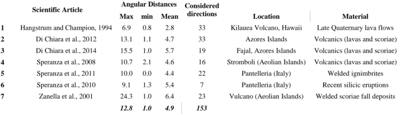
magnetic data with the best PSV curve for the sampled area. The majority of the studies that took advantage of the paleomagnetic dating and correlation technique where located at low to medium European latitudes and well constrained European PSV curves could be applied. In the Mediterranean domain, the maximum rate

of change of the magnetic field reached in the last 3000 years is 7° per 100 years (Speranza et al., 2012). Taking

an overall precision of 2-4° in measured paleomagnetic samples, this makes it possible to discriminate and

date units that emplaced within 100-200 years of one another (Speranza et al., 2012). However, a very precise

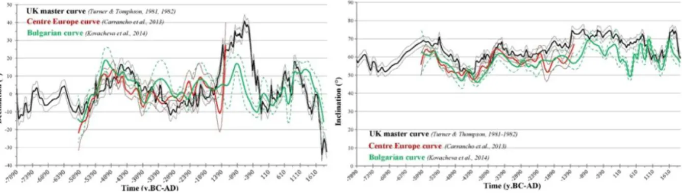
PSV curve is needed, as well as other geochronological data to provide a likely age interval, since the geomagnetic field can reoccupy the same positions through time. Such a high resolution is therefore achievable in areas where those highly precise data are present. Even though a PSV curve for Iceland does not yet exist, here I test the possibility to use some local European reference PSV curves, such as the French

Archaeomagnetic curve (0-1600 AD, Bucur, 1994; Chauvin et al., 2000; Gallet et al., 2002) and the UK master curve

(up to 8000 BC, Turner & Thompson, 1981, 1982), whose maximum distances from the study area do not exceed

2100 km. I will also make use of the Sha14k regional model (12000 bC-1900 AD, Pavón-Carrasco et al., 2014). This

model approximately covers the post-glacial period (starting from 10200 to 9000 years BP; Sigmundsson, 1991) of

emplacement of studied lavas and registers the highest precision and accuracy especially for the last 6000 y. This is a new regional geomagnetic field model based on archaeomagnetic and lava flow data (avoiding the use of lake sediment data). As this is a regional model, a new synthetic PSV curve can be compiled directly at the study location, thus avoiding the relocation error associated with the translation of local PSV curves data. This could therefore be of great help for the dating process.

Then, I will explain, analyse and test the accuracy of the chosen local reference curves transferred to

Iceland via Virtual Geomagnetic pole method (Noel & Batt, 1990) and the Sha.Dif.14k global model that

adopted dating procedure and tools follows. A final testing of the methods on historical well-known lavas is performed, in order to evaluate the potential dating accuracy of the paleomagnetic method at these latitudes.

The paleomagnetic method for correlation and dating is finally applied to a real case, taking into consideration sampled lavas erupted in the Reykjanes peninsula. Here, correlations between distant lavas are

of difficult identification, because of the very similar petrographic character (analysed by Peate et al., 2009). Age

constraints are known from literature by tephrochronology studies and archaeological deductions; nonetheless, I will apply the paleomagnetic dating method to evaluate obtained results.

2.

Paleomagnetic Sampling and Measurement

methods

ixty sites were drilled during two campaigns in July 2012 and in July 2013, in the Northern and the

Southern sections of the main rift respectively (Table 2.1 and Figure 2.1), for a total of 783 samples. In

the following paragraphs, I discuss the methods adopted for sampling, which consider the use of both traditional and innovative techniques. The laboratory methods used for acquiring the paleomagnetic information registered by collected lava samples will also be described. In situ observations, together with the paleomagnetic data analysis, suggested some consideration on which outcrops could be considered as suitable

for paleomagnetic sampling. These conclusions will be summarized in paragraph 2.3.

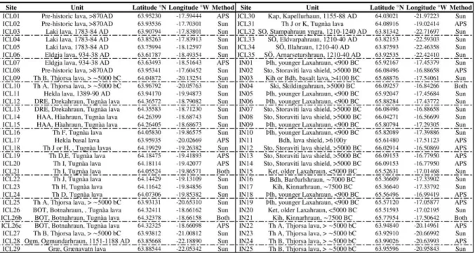
Table 2.1 Location of 2012 (ICL) and 2013 (IN) sampling sites with geological unit and emplacement age (where known from literature; Hjartarson, 2003; Saemundsson et al., 2012, 2010; Thorarinsson, 1951; Vilmundardottir et al., 1983, 1990; Vilmundardottir, 1977). Indication of the used method for calculating each

core azimuth direction is listed in column “method”: “Sun” for sun compass and “APS” for the differential GPS-laser system (see text for details).

Figure 2.1 Location of the paleomagnetic sites sampled in 2012 (ICL in Table 2.1) and in 2013 (IN in Table 2.1), with reference number. The grid coordinates are in WGS84. The names of the studied areas and the geological

units colours are indicated as they will be referred to in the following Section II, where all the details are provided.

2.1

Methods

In order to take a well-averaged and representative paleomagnetic direction of each sampling site, an average of 15 well-spaced samples (2,5-cm-diameter cores, 4-10 cm long) for each site were drilled with a

petrol-powered portable drill ( Figure 2.2). Every sampling site includes samples from in situ lava outcrops up

to 20 m wide. Each sample was not oriented in situ with the traditional magnetic compass, because the lavas object of this study are extremely magnetic and they would have strongly influenced cores azimuth

measurements. A sun compass or a differential GPS orientation system (Cromwell et al., 2013; Lawrence et al., 2009)

in cloudy weather conditions (called APS system from now on) was used, instead.

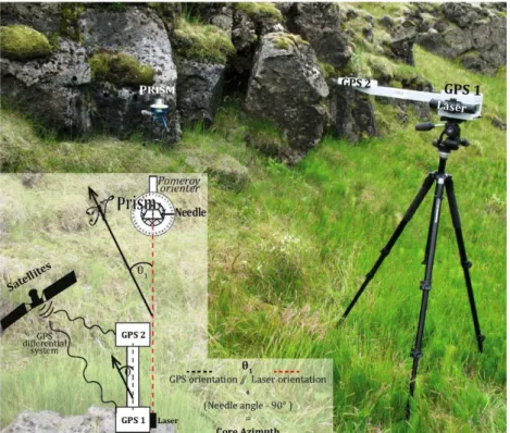
Figure 2.2 Paleomagnetic sampling. (a) Drilling with a petrol-powered portable drill; (b) measurement of in-situ samples orientation with APS differential GPS-laser system (instead of a sun compass, in cloudy conditions); (c) preparation of standard specimen for subsequent (d) measuring of the remanent magnetization

in a magnetically shielded room with a 2G DC-SQUID cryogenic magnetometer, through an alternating field (AF) cleaning in 10 demagnetization steps.

The APS system ( Figure 2.2b and Figure 2.3) constitutes an innovative orientation system, which has been initially developed by SCRIPPS Institution of Oceanography (San Diego, USA) laboratories. Recently, the INGV of Roma (Italy) perfected the instrumentation to adapt it to field working conditions, equipping it with a very stable portable tripod with bubble levels and a new rotating plate with a prism and an indicator needle mounted on the traditional Pomeroy orienter. The laser mounted on the APS is pointed towards the prism, and the latter is manually rotated until the laser hits it perpendicularly. The APS system calculates the azimuth direction of the two GPS alignment, which is parallel to the laser one. Subtracting 90° from the orientation indicated by the prism needle and then adding the APS azimuth, gives the core azimuth.

The validity of the instrument has been verified by measuring the same cores with both the instruments (sun compass and APS): differences between cores azimuth measurements are always lower than 2°, than

comparable with the 3-5° internal error of the standard paleomagnetic measurement system (Doell & Cox, 1963).

Even when sampling two sites at 500 m of distance in the same geological unit, using the solar compass in one case and the APS system in the other for orientating the drilled cores, the angular distance between the two obtained mean paleomagnetic directions is lower than 5°. As it will be explained in the following paragraphs, this degree of variability is again considered to be acceptable.

Figure 2.3 APS system or differential GPS orientation technique. The laser orientation with respect to the N (θ1),

which is perpendicular to the prism and parallel to the GPS orientation, is determined after data reduction of the GPS location and azimuth. The value indicated on the graduated ring by the needle (which is in-built with the prism, this latter rotated to be perpendicular to the laser) minus 90° and summed with the θ1 gives the core

azimuth.

It was not possible to measure the cores azimuth through the magnetic compass, because of the modifications adopted on the orienter for in-building the prism. For this reason, I could not evaluate and analyse the magnetic deflection at Icelandic locations.

Before measuring the paleomagnetic component registered by sampled lavas, core samples were cut into

standard measure specimens (2-2,5-cm-long cores, Figure 2.2.c) in order to make them compatible with the

It is important to understand that the registration of a magnetization by a rock, called Natural Remanent Magnetization (NRM), is possible because of the ferromagnetic minerals (sensu lato) dispersed in a matrix of paramagnetic and diamagnetic minerals: only ferromagnetic minerals can permanently register the direction of an applied magnetic field, by orienting parallel to this field. This magnetization is usually defined by two components: one registered during the rock formation process (primary NRM) and the other during later

events that involved the rock until the moment of sampling (secondary NRM) (Butler, 1992).

Lavas emplacement allows the registration of a type of primary magnetization called Thermal Remanent

Magnetization (TRM), which is acquired while cooling below the Curie temperature, TC. Above the TC, all the

ferromagnetic minerals are randomly oriented, but below this temperature they progressively fix parallel to the applied magnetic field: “progressively” because each grain (i.e. Single Domain grains) of ferromagnetic

mineral has a characteristic blocking temperature, Tb (lower than the TC), under which it freezes parallel to

the applied magnetic field. The acquired TRM is stable at room temperature for geologic times (unless a new

increase of temperature above the Tb occurs) and can resist to the magnetic field variations through time

(Butler, 1992).

On the other hand, an example of secondary NRM is the Viscous Remanent Magnetization (VRM) that is gradually acquired by the rock during the continual exposure to weak magnetic fields. The resultant of those

two components (a TRM and a VRM) composes the NRM vector (Butler, 1992).

The partial demagnetization techniques are able to gradually remove the NRM components; the first to be removed are the low stability components (generally representing the VRM) and their removal allows the isolation of the high stability components, which are characteristic of the NRM, or ChRM (Characteristic

Remanent Magnetization; Butler, 1992). To retrieve these components (the ChRM) from our samples, I applied

an alternating field (AF) cleaning in 10 demagnetization steps (10-150 mΤ) with a 2G DC-Squid cryogenic

magnetometer ( Figure 2.2d) in a magnetically shielded room at the INGV laboratories of Roma (Italy). This

demagnetization technique allows the simultaneous exposure of 7 samples (on the three x, y, and z axes) to an alternating magnetic field, which is a sinusoid that decreases linearly with time (time of decay is ~ 1 minute)

from the maximum applied alternating field, HAF, to zero.

Figure 2.4 Alternating-Field (AF) demagnetization scheme (modified after Butler, 1992). a) Sinusoidal waveform that decades from maximum HAF to 0 in ~1 minute. b) Detail of a) showing an example of three consecutive

sinusoid maximums: 10 mT at peak 1, -9.9 mT at peak 2 and 9.8 mT at peak 3. More details in the text. For understanding what happens during each demagnetization step, it is important to know that each

that is needed for annulling its magnetization. If a 10 mΤ HAF is applied (peak 1 in Figure 2.4b), and if we

arbitrary call this direction as the “up” direction, then all the ferromagnetic grains with coercitivity lower than 10 mT are forced to point in the “up” direction. As the sinusoid has a waveform and decreases (0.1 mT for each half cycle) with time, it will then decrease and reach a maximum in the opposite “down” direction

(peak 2 in Figure 2.4b), at 9.9 mT: here, all the ferromagnetic granules with hc lower than 9.9 mT are forced to

point “down”. When, passing again through the zero, the field reaches the new maximum 9.8 mT (peak 3 in Figure 2.4b), all granules with hc lower than 9.8 mT will point “up” again. Now, in the hc interval between 10

and 9.9 mT, all grains are pointing “up”, while in the 9.9-9.8 mT all the grains point “down”. Continuing this process until the field reaches 0 mT, the net contribution of the granules (the total magnetic moment) is

destroyed and only the NRM carried by grains with higher coercitivity (hc > HAF) is preserved (Butler, 1992). At

the end of each AF cleaning step, then, the NRM component is measured by the magnetometer, so that when all the steps are completed we are able to analyze the ChRM.

In some cases, a thermal demagnetization has been carried out, with 10 demagnetization steps from 200 to 600°C. This type of demagnetization process allows a heating of samples to an elevated temperature (each step higher), then a cooling to room temperature within a non-magnetic environment. All ferromagnetic minerals

with a blocking temperature, Tb, lower than the applied temperature will have their original NRM erased.

Measuring the magnetization after each heating step will record the unaltered ChRM, which has been

registered by ferromagnetic minerals with higher Tb. In general, NRM components that are easily and rapidly

removed during early demagnetization steps are called low temperature (LT) components, while the high-temperature (HT) components resist to higher demagnetization steps. These HT components generally represent the ChRM.

Both the AF cleaning and the thermal demagnetization steps were carried out until 150 mT and 600° C respectively, in order to reach a significantly low magnetization value, which indicates the complete demagnetization of the magnetic minerals. This allows the identification of the real ChRM.

Data obtained from those different demagnetization process can be plotted on both orthogonal

demagnetization diagrams (Zijderveld, 1967) and on equal areal projections (the Lamber or Schmidt projection,

as denoted in the used Remasoft software of Chadima & Hrouda, 2006) as shown in Figure 2.5. Each point from 0

to 6, representing a step of the demagnetization process, is indicating the tip of the NRM vector measured at

that particular step, starting at 0,0 coordinates. From c. and f., it is clear that the more unstable VRM

component can be recognized because of its variation in inclination and declination, while the more stable ChRM component maintains the same declination and inclination (with a straight trajectory towards the

Figure 2.5 (Modified after Butler, 1992) a,b) Three dimensional diagrams that show the behaviour of the NRM vector during a demagnetization process, from step 0 (original conditions) to step 6 (maximum heating temperature or alternating-field applied). Each step in all the following diagrams will be represented by a single

point, but this tridimensional diagrams let us understand that in reality each point is the tip of the registered NRM vector at that step, which originates from 0,0 coordinates. The dashed line represents the low stability component (VRM) while the solid line is the high stability ChRM, which decreases in intensity (c) but does not change its direction. c) NRM intensity (Jr) diagram that shows a decrease during each demagnetization step. d)

Equal area projection (lower hemisphere) and its three dimensional explanation. In the projection it is clear that the direction of the NRM vector changes from step 0 to 3, but remains stable from 3 to 6. e) Representation of

the variations in declination and inclination of the NRMs through the demagnetization process on a two dimensional Cartesian plane. f) Zijderveld diagram obtained by the fusion of the diagrams in e). It is possible to calculate the linear trajectories that best fit those components through the Principal

Component Analysis (PCA), which also gives a statistical estimate (Fisher statistics, see Appendix II) of the

reliability of the data with a 95% confidence limit (α95). This mean error, α95, is expressed in degrees and

indicates the cone of confidence in which the real paleomagnetic direction could lie (the maximum angular

deviation).

The fact that more than one component can be identified is particularly important for thermal demagnetized data, because the presence of multiple components can indicate a re-heating of the sampled rock. The thermal demagnetization steps between which the changing in components direction happens are indicative of the temperature reached by the lava because of this re-heating.

2.2

Data Analysis and in-situ Observations

Following the procedures listed in the previous paragraph, I obtained a mean paleomagnetic direction for all the sampled cores. I applied the thermal demagnetization process on some samples (ICL05, ICL13, ICL14,

ICL26, IN05) that showed a high intensity of magnetization (~3 x 10-2), which caused errors in the cryogenic

magnetometer measures. In those cases, after the 200°C step of heating, the samples intensities were in ranges that could be measured by the magnetometer and the demagnetization process could be continued.

Sites paleomagnetic directions were obtained by applying the PCA to each of the 783 measured cores and then averaging the ChRM obtained for the cores pertaining to the same sampling site using the Remasoft 3.0

browser and analyser (Chadima & Hrouda, 2006). The averaged mean paleomagnetic direction calculated for

each site is weighted by the quality of the cores directions (α95) that have been averaged to obtain each site

projection in Figure 2.6, where the α95 is represented by the grey circle surrounding each mean direction.

These data and projections were analysed and obtained through the Remasoft 3.0 browser.

Table 2.2 Table showing the mean paleomagnetic directions for sampled site: Site, number of averaged cores on the total number of cores (n/N), declination (D) and inclination (I), degree of clustering of the directions (k) and

estimate of the precision of the calculated mean direction (α95). The gray-coloured sites paleomagnetic

Figure 2.6 Lower hemisphere, equal-area projection of all the sampled data mean paleomagnetic direction, with their α95 indicated as a gray circle. 2012 ICL drilled samples are indicated with italic numbers, while 2013 IN

samples are in bold characters. Geological units of each sample are listed in legend and refer to the Table 2.1 “Unit” column.

Some observations can be made. The first consideration is focused on the reliability of the data: results

show that the α95 is mainly lower than 5° for each site, ranging from 1.7 to 5.1°, which is comparable to the

3°-5° internal error of the paleomagnetic sampling and measuring method (Doell & Cox, 1963). As each site mean

comes from the averaging of each specimen ChRM, the obtained α95 also testifies to a strong internal

consistency for each site. Only 7 out of 60 paleomagnetic sites means have been rejected (light gray in table 2)

because the calculation of the paleomagnetic mean has not been possible due to the high scattering of the cores ChRMs or, either, because their ChRM did not correspond to a possible/real paleomagnetic direction. This may be due to a serious tilting of the sampled lava that brought the paleomagnetic direction to show highly unrealistic values of declination (D) and inclination (I) with respect to the values acquired, for example, by the Earth’s magnetic field in the last 12’000 years. The term “unrealist” indicates that the D and I values were NEVER similar to the ones acquired by the Earth’s magnetic field, even considering a 20° tolerance about the present and past directions.

The second consideration comes from plotting the sites ChRMs on the Zijderveld diagram. The majority of

the samples shows a single marked ChRM component since 20 mΤ (Figure 2.7) that resolutely points towards

the origin, suggesting that magnetic fields applied after the cooling had little to no influence for the registration of low temperature components in studied lavas. In general, only the first step of the demagnetization process was discarded.

Figure 2.7 Four representative orthogonal vector diagrams (Zijderveld, 1967) of alternating-field (AF) demagnetized data. Declination and Inclination values obtained from the Principal Component analysis, together with the MAD, Maximum angle of deviation, are indicated. The complete list of diagrams for all the

sampled sites has been added as Appendix II.

Other considerations arose during the sampling and became evident while analysing the obtained ChRM. To explain them I must start by realizing that the areas where Icelandic post-glacial volcanic activity has developed have undergone a very limited fluvial erosion so that wide roof surfaces of shield basalt lava tubes, internal walls of lava tubes and rootless scoria cones prevail. It follows that only where rivers or waterfalls have exposed the inner massive part of the lava, can the paleomagnetic sampling be done without problems (Figure 2.13b). But as in Icelandic post-glacial domains these sites are relatively rare and mainly cracked and tilted lava tubes prevail, I wondered whether there was the possibility to take advantage of other sampling options.

I decided to sample both in roofs and tilted flanks of lava tubes, drilling in the most internal available part of the crust, where the higher temperature provided by the under-flowing hot lava could have preserved a TRM even during the tilting of the lava tube crust. In that case, the HT (high temperature) component of both the tilted flank and the roof of the lava tube would share the same paleomagnetic direction, and the transition to a LT ( low temperature) tilted component would provide the temperature at which the heating (and the registration of the HT component) of this tilted part of the crust had occurred.

For better understanding if this reasoning was correct, I also drilled a series of cores along a tilted flank of a lava tube in order to obtain a profile of the NRM variation through it. The experiment was meant to observe what consequences on the NRM had a new inflation of a hot lava into a cooled lava tube. As it is sketched in Figure 2.8, the already cooled lava tube would have cracked and tilted, but because of the reheating of the internal crust I expected to observe also a gradual reorientation of the tilted NRM (from a scattered

component in Figure 2.8b point 3, to a double component, a re-heated HT one and a tilted LT one in point 2)

parallel to the magnetic field and to the one registered by the massive core of the inflated lava (HT component in point 1). If this was true, a sampling in the most inner part of whatever crust, would have registered a trustworthy HT component of the magnetization.

Figure 2.8 The emplaced lava cools down and registers the paleomagnetic direction of the acting magnetic field. If a new inflation of lava occurs, the solidified crust can crack and tilt, rotating the previously registered

paleomagnetic component. This component can be re-oriented parallel to the magnetic field only if the temperature in the cold crust increases enough for the magnetic minerals to be free to “move” and re-orient.

Higher temperature is supplied by newly inflated lava.

I performed an additional thermal demagnetization of the cores of sites sampled in lava tube tilted flanks or roofs (using a new unmeasured specimen from each core). The analysis of results shows that sampling in lava tubes can give various outcomes. It is possible to identify the presence of more than one TRM component, representing an original and a tilted paleomagnetic direction, and the temperature at which the tilting (between these components) occurred. The tilting must have occurred at temperatures lower than the ones at

which the transition from one component to another happens. In Figure 2.9, we can see that the majority

(85%) of the 65 cores measured through the thermal demagnetization process showed a single marked component since the very first steps of the demagnetization (20°-200° C). Only the 11% of the samples showed a LT component between room temperature and the 300°C step of the demagnetization, and a HT component from 300° to 600°C. Only 4% of the samples shows a better distinction between the two components, with a tilting temperature ranging between 300° and 450°C.

Since the majority of the cores shows a single component, it is important to be sure that this is a non-tilted, reliable ChRM. For this reason, it is even more important to chose a reliable sampling location.

Figure 2.9 Frequency histograms of the maximum temperature at which the tilting between the HT and the LT components occurred. This temperature is identified by analyzing at which temperature step of the demagnetization process lies the kink between these two components. 65 cores where analyzed and represent the

100%.

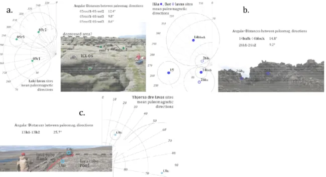
Samples collected in different blocks of lava tubes roof (Figure 2.10a, 5 cores have been drilled in each

block, r1-r2-r3) indeed show scattered paleomagnetic means with angular distances between 8.6° and 12.4°,

which are too high to take their overall site mean as reliable. As I will explain in detail, only when two paleomagnetic direction have an angular distance <10°, I consider them as pertaining to the same unit. In

other cores, where tilted blocks and roofs of the lava tubes where sampled (Figure 2.10b and c), the angular

distances between cores sampled in the tilted parts and in the roof zones are again higher than 9°. In those cases, statistical observations of these sites’ paleomagnetic means could not guarantee for their reliability.

67.7% 16.9% 1.5% 7.7% 1.5% 1.5% 1.5% 1.5% max tilting T < 20° max tilting T < 200° max tilting T < 250° 200°< max tilting T < 250° 250°< max tilting T < 300° 300°< max tilting T < 350° 350°< max tilting T < 400° 400°< max tilting T < 450°

Figure 2.10 Examples of a) tilted lava roof blocks and lateral cracks emptying lava tubes (sites ICL14, ICL26 and ICL13)

bear a high angular distance value, so that most of those data were discarded in further analysis. In some cases, very wide lava tubes (at least 10

appeared to preserve blocks continuity

even if sampled in different areas of the roof ( sampled core appears to be very stable,

Figure 2.11 Sites IN 15 and IN 20, sampled on the top of a large and extremely well preserved lava tube, with the paleomagnetic directions of each sampled c

Examples of a) tilted lava roof blocks and lateral cracks (site ICL05)

(sites ICL14, ICL26 and ICL13). The relative paleomagnetic directions are scattered and angular distance value, so that most of those data were discarded in further analysis.

very wide lava tubes (at least 10-15 m) still showed a perfectly preserved shape and cracking

appeared to preserve blocks continuity (Figure 2.11). At these sites, paleomagnetic data show a high reliability

even if sampled in different areas of the roof (Figure 2.11), the paleomagnetic direction registered by each

ore appears to be very stable, within each site.

Sites IN 15 and IN 20, sampled on the top of a large and extremely well preserved lava tube, with the paleomagnetic directions of each sampled core on a equal-area projection (lower hemisphere). For each

and of b,c) inflating or . The relative paleomagnetic directions are scattered and angular distance value, so that most of those data were discarded in further analysis.

15 m) still showed a perfectly preserved shape and cracking aleomagnetic data show a high reliability; he paleomagnetic direction registered by each

Sites IN 15 and IN 20, sampled on the top of a large and extremely well preserved lava tube, with area projection (lower hemisphere). For each

site, samples were taken in three different and distant locations, but their paleomagnetic values are comparable and well averaged by the sites means (α95 are 3.5°and 1.8°, respectively).

From these observations and paleomagnetic results (Figure 2.10Figure 2.11), it is clear that the lava tubes

crust tilting could have happened during the cooling itself. It becomes of crucial importance to verify if the inner part of the crust of lava tubes, being in close contact with the hot lava underneath, maintained or regained the record of the original magnetic field direction. As discussed previously, the two thermal profiles

(IN07, IN14, Table 2.2) from the surface of tilted crusts to the not-tilted internal massive cores were completed

through 2 tilted lava tubes. The aim was to verify if the paleomagnetic direction registered in the inner part of a tilted crust was identical to the one registered by in-place massive lava even after a tilting had occurred. The massive lava core was sampled as a new and independent paleomagnetic site: IN02 as reference for profile IN07, and IN13 for profile IN14. Determining the Low and High temperature components for the 23 cores pertaining to the thermally demagnetized cores profiles allow the identification of the temperature at which the transition happened. Such transition indicates a temperature that was high enough to register again an un-tilted paleomagnetic component.

Detailed results shown in Figure 2.12 illustrate that temperature in those tilted crusts decreases abruptly in

the first 50 cm from the inner part and that, after this thin re-heated part, the only paleomagnetic component registered by the crust is the tilted one. The maximum heating temperature reached in those 50 cm is 300-440°C, enough to register once again the paleomagnetic field direction. So, the non-tilted NRM primary component is effectively registered only by lavas in very close proximity to the massive core of the lava tube.

Figure 2.12 Paleomagnetic sampling through lava tubes crust: moving progressively into the inner part of the tilted crust, the registered tilted component becomes a two components (low LT, tilted and high HT, non-tilted component), until only the high temperature non-tilted component is recorded. The changing between the tilted

and non-tilted component happens between 260-440° C in the first 50 cm from the massive core of the lava. More details on the demagnetization process in Appendix II.

As Iceland is rich in water, such as streams, rivers, lakes, marshes etc., it is common to find fields of rootless scoria cones within the lava flows; a hot lava flowing on a wet area causes the formation of water vapour that, trapped below the lava, reaches a pressure high enough to break the lava crust, generating a

localized eruption and the formation of those rootless scoria cones (as described in Thorarinsson, 1951). This

happens particularly when lava flows reach the lowlands facing the ocean, or other depressed and water-rich areas. If those features are found in place and well-preserved, their own origin would suggest that the

paleomagnetic information registered during the cooling might not be changed through time (Figure 2.13.a),

as they do not move with the lava flow, once formed. The same reasoning could be applied to the internal wall

of an emptied lava tube (Figure 2.13.c) that shows vertical slickensides, where the subsiding part of the crust

has rubbed against and scratched the wall in its descent, and horizontal ones, where the crust had halted long

enough to become attached to the still plastic mass (Thorarinsson, 1951, 1979). Here too, a well-preserved site

would suggest that the NRM component is reliable.

A total of 7 paleomagnetic sites have been sampled in these conditions: 5 sites in rootless scoria cones and 2 in the internal wall of lava tubes.

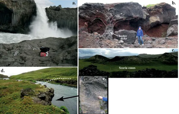
Figure 2.13 Alternative sites chosen for paleomagnetic sampling: a) massive lava core exposed by a waterfall (site IN 17); b) section of rootless scoria cone, with visible feeding dyke (site IN 01); c) well-preserved rootless

scoria cones; d) internal part of a lava tube (whose roof would be located where the dashed white line indicates), now occupied by a river (site IN 09), with e) slicken-lines on the internal wall.

Two of the sites sampled in rootless cones have been rejected. In one case (IN 05) it was not possible to calculate the NRM through the PCA analysis because of the high scattering of the data, while in the other case (IN 06) the site paleomagnetic mean resulted in an unrealistic direction with respect to the directions obtained in other sites sampled in the same unit (e.g. IN 9 and IN 19). This was probably due to a serious tilting occurred at the small rootless cone chosen as sampling location, so that such small cones won’t be sampled in

the future. On the other hand, where the feeding dyke could still be identifiedd and sampled (IN 01 in Figure

2.13b, IN 10, IN18), paleomagnetic results gave consistent results with an α95 of 2.9°, 2.6° and 3°, respectively.

Sites sampled in the internal wall of lava tubes (IN 9 in Figure 2.13d,e and IN 19) gave, once again, consistent

results, as their paleomagnetic means bear an α95 of 2.3° and 2.2°, respectively.

2.3

Discussions

Throughout this research, both traditional and innovative paleomagnetic techniques have been used. Here, the apparent typical paleomagnetic sampling techniques met some uncommon obstacles, from the absence of sun for the sun compass orientation of drilled cores, to the lack of suitable outcrops for sampling.

Through the use and validation of the APS system for orientating drilled cores and the choice of alternative sampling sites, those obstacles have been successfully overcome, giving the possibility to continue the research.

Obtained data show the high consistency of paleomagnetic directions, whose reliability at 95% confidence

limit (α95) never exceed 5.1°. Furthermore, paleomagnetic means from all the sites indicate the presence of a

single ChRM component, stable since the very first steps of AF and thermal demagnetizations. These results lead us to the understanding of which sites could be indicated as suitable for paleomagnetic sampling.

In Iceland, where massive outcrops are rare because of a limited fluvial erosion on many Holocene lavas, I tested the reliability of other sampling site types. Both well-preserved rootless cones and internal walls of lava

tubes have proved to be trustworthy and therefore to be excellent sampling sites, as their own origin guarantees that their position has not been tilted through time.

On the other hand, lava tube roofs, although widespread and the most common outcrops to be found, need to be treated more carefully, as they could easily have been moved and tilted, causing a rotation of the original direction of the magnetic field acting during the emplacement and registered by the lava during the cooling. Results indicate that the tilting mostly occurs when the crust is already at temperatures lower than 250°C (Figure 2.9), thus mainly showing only the tilted component of the NRM.

Paleomagnetic data show that, where lava tubes are small (less than 10 m), not well preserved, or present a too much pronounced tilting of the flanks or depression of the central area, the resulting paleomagnetic directions of different blocks are scattered, and because of this inconsistency within the same site, they have

to be discarded (Figure 2.10). On the other hand, very large (at least 10-15 m), well preserved lava tubes prove

to maintain their continuity between cracked blocks, preserving their original NRM without tilting (Figure

2.11).

A more detailed study of the variation of the NRM components within a tilted lava crust profile helped in verifying that a new inflation of lava can cause the cracking and tilting of a cold crust but, at the same time, it can provide a temperature high enough for the tilted crust to partially re-orient the tilted paleomagnetic

vector in the “correct” position (Figure 2.12). From our study, this re-heating only occurs in the first 50 cm of

the inner crust, registering a maximum re-heating temperature of 300-440°C. In such a case, even if only tilted or not well preserved lava tubes can be found, a sampling in the inner part of the crust, as near as possible to the massive core, would be reliable for paleomagnetic purposes. However, it is clearly fundamental to sample in the massive core or in its close proximity.

On the whole, the simple initial activity of sampling and measuring the paleomagnetic directions registered by studied lavas gave a lot of new and useful information on the method itself.