Socioeconomic status and net fertility
in the demographic transition:
Sweden in 1900 – A preliminary analysis
*F R A N C E S C O S C A L O N E , M A R T I N D R I B E Lund University
1. Introduction. The decline of fertility in the demographic transition has for a long time been a major theme in historical demography. Much of the literature has focused on the demographic aspects of the decline, aiming to chart the process without actually explaining it. Other research has offered explanations for the decline mainly at the macro level, and making distinctions between innovation and adjustment processes as causal agents in the decline. Much less attention has been given to disaggregated patterns and micro-level analyses.
One of the issues of great relevance for understanding the fertility decline is the differences in fertility according to socioeconomic status, and how these differences evolved over the fertility transition. There appears to be a generally accepted view that high social status was associated with high fertility in pre-transitional society but that this situation reversed during the transition, or even before (Skirbekk 2008; Livi-Bacci 1986). This change has been explained by the higher social groups act-ing as forerunners in the decline (Livi-Bacci 1986, Haines 1992) but it remains unclear whether the change happened because new incentives were affecting the elite groups first (adjustment) or if it had to do with a diffusion of new ideas first adopted in these high-status groups (innovation) (see Haines 1992).
Part of the difference between socioeconomic groups in terms of fertility was also related to spatial differences in socioeconomic structure, rather than to social status as such (Garrett et al. 2001), making it vital to control for this aspect when analyzing socioeconomic stratification and fertility in national populations (see also Szreter 1996).
The aim of this paper is to study the socioeconomic differentials in fertility dur-ing the transition. We use data from the Swedish census of 1900 coverdur-ing the entire population (about 5 million individuals), which makes it possible to look at the socioeconomic pattern in considerable detail while controlling for spatial hetero-geneity. We also estimate a model of fertility including control variables at the indi-vidual, household and community level. This is a preliminary study looking only at one census. Later revisions will add data from 1880 and 1890, and also link indi-viduals between censuses, which will make it possible to study more of the dynam-ics of this process.
*This work is part of the project «Towards the modern family. Socioeconomic stratification, fam-ily formation and fertility in a historical perspective», funded by the Swedish Research Council and the Crafoord Foundation.
The great advantage of census data is the coverage and the possibility of study-ing fertility differentials by socioeconomic status across space without problems of small sample size. They also offer quite detailed information on occupation allow-ing classification into a fairly large number of social groups usallow-ing the HISCLASS
scheme (Van Leeuwen, Maas 2011). The main disadvantage with census data is that it (at present) only offers the possibility of a cross-sectional perspective. Further, we lack data to compute standard fertility rates (ASFR, TFR, etc.) and instead have to
rely on indirect measures such as the child-woman ratios.
The first part of this paper provides a brief background on the fertility transi-tion in Sweden and summarizes the main analytical framework for studying socioe-conomic differences in reproductive behavior. A description of the structure of the census data is followed by some indirect estimates of fertility by socioeconomic sta-tus and the main empirical analysis.
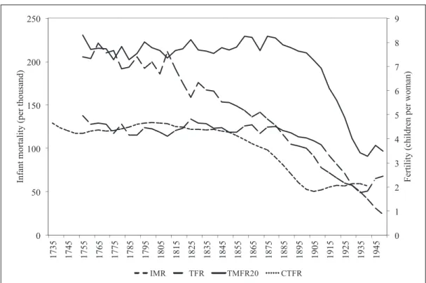
2. Background. We begin by looking at fertility developments in Sweden over a long period from the early eighteenth century until 1950. Figure 1 displays the infant mortality rate (IMR), period total fertility (TFR) and total marital fertility for
women over 20 (TMFR20) as five-year averages, as well as accumulated fertility at
0 1 2 3 4 5 6 7 8 9 0 50 100 150 200 250 1735 1745 1755 1765 1775 1785 1795 1805 1815 1825 1835 1845 1855 1865 1875 1885 1895 1905 1915 1925 1935 1945 Fe rti lit y ( ch ild re n p er w om an ) In fa nt m or ta lit y ( pe r t ho us an d)
Fig. 1. Period and cohort fertility and infant mortality in Sweden (1735-1950)
Source: Statistics Sweden 1999, Table 3.3, 3.4, 3.7 and 5.1.
Note: IMR= Infant mortality rate (per thousand). TFR= Period total fertility rate. TMFR20 = Period total
marital fertility rate in ages over 20. CFR= Accumulated cohort fertility rate at age 50.
Labels on the x-axis refer to the ending year in quinquennial rates for IMR, TFRand TMFR20 (1751-1755,
1756-1760, etc.), and year of birth for CFR.
age 50 by birth cohort (CFR). Despite some medium-term fluctuations the
long-term level of fertility was quite stable until the last quarter of the nineteenth centu-ry; between four and five children per woman, or around eight children for married women. Beginning around 1880 period fertility started to decline steadily until the beginning of the 1930s when it started to increase again. Between 1880 and 1900 the decline was modest, but gained considerable speed thereafter. This period, between 1880 and 1930, marks the first phase of the decline of Swedish fertility. It constitutes an important phase of the demographic transition, about 100 years after infant mortality started its continuous decline. Looking at the cohort fertility pat-tern the decline starts from the cohorts born around 1850, in other words women who were in prime childbearing ages in the early 1880s when period fertility start-ed to decline.
Marital fertility follows closely total fertility, showing that the decline can main-ly be attributed to a decline in marital fertility rather than changes in nuptiality, which is also a well-established conclusion from previous research on the European fertility transition (Carlsson 1966; Coale, Watkins 1986). The fertility of the oldest age groups declined fastest, even though the decline started in all age groups over 25 at about the same time (see Dribe 2009). In terms of the relative contribution of different age groups to fertility decline it was also the prime childbearing ages (25-40) that contributed most to the decline. Just before the fertility transition most counties in Sweden did not show any signs of parity specific control, which implies that, with a few exceptions, the fertility pattern in pre-transitional Sweden can be characterized as natural (Henry 1961). Nonetheless, the level of marital fertility var-ied quite a lot between counties and these differences not only persisted during the transition but actually widened in relative terms (Dribe 2009).
A previous study on the determinants of fertility decline using county level data (Dribe 2009) showed that fertility decline in Sweden was associated with both the demand for and the supply of children, and is in line with the Easterlin-Crimmins framework (Easterlin, Crimmins 1985). A higher supply of children following lower child mortality was associated with lower marital fertility. Higher urbanization and stronger educational orientation were also associated with lower fertility, as they were both related to higher costs and the lower economic benefits of children. Similarly, increasing female relative wages were associated with declining fertility among women over 35, which is consistent with higher opportunity costs of having children when women’s earning potentials increase. It is also clear that older women in Sweden adjusted their fertility behavior more profoundly than younger women, but all age groups were affected by socioeconomic and demographic change. Moreover attitudes towards birth control may have played an important role as shown by the cross-sectional effects of the proportion of socialist voters on marital fertility in all age groups (Dribe 2009). Similar patterns have been shown for different parts of Germany (Brown, Guinnane 2002; Galloway, Hammel, Lee 1994).
So, previous research tends to support an interpretation that connects fertility decline with broad socioeconomic changes taking place in the late nineteenth and
early twentieth century following the transition from an agriculturally based econ-omy to an industrial one. This transition involved sustained mortality decline, increasing levels of urbanization, expansion of education and increased female par-ticipation in the labour market. The question remains how these changes affected different socioeconomic groups?
Looking at the fertility decline in France, Germany, Britain, Norway and the United States Haines (1992) showed that the socioeconomic differentials, as mea-sured by occupation, generally widened during the transition. Fertility decline in all these countries except France was led by the middle and upper classes, while the agrarian population was slower to change. The question is whether this pattern was the result of socioeconomic change which first affected the upper and middle class-es and only later hit the lower classclass-es as well, or if it was part of an older pattern whereby innovation diffusion from upper to lower social strata.
According to Livi-Bacci (1986), European elite groups often acted as forerun-ners in the fertility transition, showing declining fertility quite a long time before the general decline in fertility. He also argued that, in part at least, the early decline of these groups was connected to urban residence, but it remained uncertain whether it was urban life as such that created special preconditions for fertility decline, or if it was rather something more specific to the elite groups as such.
There is also evidence from other studies pointing in the same direction. High status families in pre-transitional Sicily had considerably more surviving children than low status families which was explained by a combination of mortality and higher mar-ital fertility (shorter birth intervals) (Schneider, Schneider 1996). In the decline the higher social groups acted as forerunners with the poorer groups lagging behind. However, looking at Stockholm in the period immediately after the fertility decline in the 1930s, Edin and Hutchinson (1935) found higher marital fertility for higher status groups, regardless of whether status was measured by occupation, wealth or education. It remains unclear if these results are specific to the capital city or can be generalized to the country as a whole. In pre-transitional Norway, on the other hand socioeco-nomic fertility differentials were quite modest, with somewhat higher fertility (about 10%) in the highest status group (but unclear if the difference is statistically signifi-cant), and more or less identical rates in the middle and low status groups (Sogner, Randsborg, Fure 1984). Nonetheless, the fertility decline started in the higher social groups and then spread to the lower status groups.
In his study of socioeconomic fertility differentials in Britain during the fertility decline using the 1911 census, Szreter (1996) stressed the interplay between geog-raphy and class in the decline. Fertility decline was not simply diffused socially and geographically following a certain pattern. Instead, there were pronounced differ-ences within different social groups regionally, having to do with differdiffer-ences in the perceived costs of child rearing. As conditions changed new attitudes and values spread within these regional social groups by way of changing discourse. This change in discourse, however, could in turn to a large extent be determined by changing economic conditions.
gained renewed attention by economic historians following the publication of Clark’s A Farewell to Alms (2007). Based on data from wills he shows that the num-ber of surviving children was higher among richer people in preindustrial England, but also that these differences diminished well before the fertility transition (see also Clark, Cummins 2009; Clark, Hamilton 2006) and similar findings have been made for France (Cummins 2009) as well as for England using occupational data from family reconstitutions (Boberg-Fazlic et al. 2011).
From a theoretical point of view, fertility decline is often viewed within a frame-work of innovation and adjustment (Carlsson 1966), where the first explains fertil-ity decline as a result of new knowledge or attitudes to fertilfertil-ity control, while the latter sees the decline as a result of an adjustment of behavior to new circumstances and a greater motivation to limit fertility. In an alternative, but equally classic, for-mulation, Coale (1973, later developed by Lesthaeghe, Vanderhoeft 2001) identi-fied three conditions for fertility decline, namely that people needed to be ‘ready, willing and able’. These three conditions involve both adjustment and innovation.
According to the innovation perspective, fertility before the decline was not deliberately controlled, but ‘natural’ (Henry 1961). Thus, marital fertility was not affected by parity-specific stopping but determined by the length of birth intervals, and these in turn were to a large extent determined by the length of breastfeeding and the level of infant and early child mortality. According to this perspective the fertility decline was mainly a result of the innovation of families to start limiting family size by terminating childbearing after having reached a target family size (Coale, Watkins 1986; Knodel, van de Walle 1979; Cleland, Wilson 1987). In the words of Coale (1973), fertility came «within the calculus of conscious choice», which, it seems to be implied, was not the case before the transition. The emergence of deliberate birth control involved cultural transmission of new ideas and chang-ing attitudes and norms concernchang-ing the appropriateness of fertility control within marriage. It also involved acquiring knowledge of how to limit fertility, but many believe this knowledge to have been present long before the decline even though it might not have been used for parity-specific control, but for spacing of births or avoiding childbearing in difficult times (see, e.g. Bengtsson, Dribe 2006; David, Sanderson 1986; Dribe, Scalone 2010; Santow 1995; Szreter 1996; Van Bavel 2004).
One might expect that higher social groups would be more likely to formulate and adopt these new ideas as they were culturally more open and increasingly felt it important to distinguish themselves from the lower classes. Such a strategy of dis-tinction in the middle class has been shown to be important for other aspects of family life, for instance in marriage patterns (see Van de Putte 2007; see also Frykman, Löfgren 1978). The middle class and elite groups can also be expected to have been better able to acquire new knowledge about methods of birth control to the extent that these were not generally known before. In other words, provided that innovation was important for the decline in fertility, which after all has been the orthodoxy of historical demography for quite some time, we would expect high social status to be connected to early fertility decline (Cleland 2001).
to changes in the motivation for having children. In the theoretical framework out-lined by Easterlin and Crimmins (1985), both the demand for and the supply of children are important in explaining the high pre-transitional fertility. The supply of children is defined as the number of surviving children a couple would get if they made no conscious efforts to limit the size of the family (Easterlin, Crimmins 1985). Thus, it reflects natural fertility as well as child survival. High mortality in pre-tran-sitional society (low supply) together with a high demand for children implied that demand exceeded supply. Following the mortality decline the supply of children increased which contributed to the decline in fertility (Galloway, Lee, Hammel 1998; Reher 1999; Reher, Sanz-Gimeno 2007). However, declining mortality was only part of the explanation as fertility was reduced much more than mortality which implies that fertility decline also involved the number of surviving children, or in other words in net fertility (Doepke 2005).
This means that a changing demand for children also was important for the fer-tility decline (Brown, Guinnane 2002; Galloway, Hammel, Lee 1994; Dribe 2009; Mosk 1983; Schultz 1985; Crafts 1984). The demand for children can be defined as the number of children a couple would want if there were no costs to limiting fer-tility, depending on family income and the cost of children in relation to other goods that are directly related to social status, economic conditions and occupa-tional levels. Following industrialization and urbanization the motivation to have children changed, and this can be expected to have affected socioeconomic groups differently. On the one hand, higher consumption aspirations among high status groups would have increased the opportunity cost of childbearing and therefore contributed to a reduced demand for children. On the other hand, since children could help out working in the fields or assisting in supplementary activities, from a relatively early age, the economic benefits of children might also have been higher among low and middle class families in rural contexts, implying a delayed response in terms of fertility decline in these groups.
In addition, as industrialization and urbanization increased the returns to edu-cation, demand for child quality also increased (Becker 1991). This led families to substitute quantity for quality, by having fewer children and investing more in each child. This quantity quality trade-off has been viewed as an important explanation for the decline in fertility (Dribe 2009; Wahl 1992) as well as for the escape from the Malthusian trap and the emergence of modern economic growth (Galor 2005; Becker et al. 2010).
Empirical studies have also confirmed that smaller family sizes in the demo-graphic transition became increasing connected to upward social mobility for chil-dren (Van Bavel 2006; Van Bavel et al. 2011; Bras, Kok, Mandemakers 2010). It could be expected that this change towards more investments in child quality would first be adopted by the higher status groups, partly because of a higher return to education in these occupations and partly because of better knowledge and information about the new conditions emerging in these socioeconomic groups.
fer-tility and socioeconomic status before the ferfer-tility transition, at least in terms of total fertility (for marital fertility this is less clear). More relevant for this study, how-ever, we should expect an earlier decline among the higher status groups leading to lower fertility in these groups early in the transition. Moreover, we expect substan-tial geographical differences in the fertility decline both between different regions and between urban and rural areas. Because the patterns of socioeconomic stratifi-cation also differ regionally, socioeconomic differentials will be smaller when also taking the spatial patterns into account.
3. Data. The present study uses data from the 1900 census of Sweden. Historically Swedish censuses were carried out differently from most other countries. Instead of collecting information from people interviewed in their homes, data collection was made by parish priests who extracted the necessary information directly from parish record books. In total, the 1900 census counts 5,200,111 persons and 1,433,206 households. Geographically, these data are from 2,533 geographical units (most often parishes) grouped in 24 counties.
The micro census data were digitalized by the Swedish National Archives and were downloaded from the North Atlantic Population Project (NAPP) database
(Ruggles et al. 2011; Sobek et al. 2011) which adopts the same format of the Integrated Public Use Microdata Series (IPUMS)1. All registered individuals are
grouped by household. In this way, each individual record reports the household index number and the person index within the household. The age, marital status and sex of each person are also registered. Migration status indicates if a person was born in the same county of residence or in another county or country. A person’s relationship to the household head is also recorded. In addition, there are family pointer variables indicating the personal number within the household of the moth-er, fathmoth-er, or spouse, making it possible to link each woman to her own children and husband. It is also possible to link children to their step-mother/aunt/grandmoth-er or to exclude them if necessary. According to the NAPP-IPUMS structure, each
record provides additional information about the characteristics of the household in which the person lives (number of servants, children under 5 or other families).
We follow a long tradition in social stratification research in using occupation as the core information to identify socioeconomic status (Van Leeuwen, Maas 2010). In the census data individual occupations were coded according to the Historical International Standard Classification of Occupations (HISCO) (Van Leeuwen, Maas,
Miles 2002). Based on HISCO we have classified occupations into different classes
following HISCLASS (Van Leeuven, Maas 2011)2, which is a 12-category
classifica-tion scheme based on skill level, degree of supervision, whether manual or non-manual, and whether urban or rural. It contains the following classes: 1) Higher managers, 2) Higher professionals, 3) Lower managers, 4) Lower professionals, and clerical and sales personnel, 5) Lower clerical and sales personnel, 6) Foremen, 7) Medium skilled workers, 8) Farmers and fishermen, 9) Lower skilled workers, 10) Lower skilled farm workers, 11) Unskilled workers, 12) Unskilled farm workers.
identifies whether a person aged 15 and above reports any gainful occupation. Finally, parish and county of residence are also available. Therefore, by aggregating the data at parish or county levels, it is possible to calculate community-level socioe-conomic indicators, for example rates of industrialization, education or migration. 4. Indirect estimates by socioeconomic status. For Sweden in this period we have data to calculate age-specific fertility (both total and by marital status) at national and county levels. However, these kinds of detailed demographic data are not avail-able by socioeconomic status. Only in the census can we find nation-wide data on occupation at individual level. Because census data do not permit the computation of standard fertility rates (ASFR, TFR, etc.), indirect measures such as the
child-woman ratios (henceforth CWRs) and the own-children method (OCM) have to be
used.
The CWRhas been traditionally defined as the number of children aged 0-4 per
1,000 women aged 15-49 (Shryock, Siegel 1980). It is easy to see that children under 5 may have been born during the 5-year period before the census date, where the women were up to 5 years younger. If micro census or household list data are also available, it is possible to apply the own-children method. This method is based on measuring the medium-term consequences in the age structure caused by the fertility trends and in effect works as a reverse-survival technique, producing total and age-specific fertility rates for the fifteen years before the census (Cho et al. 1986; UN1983).
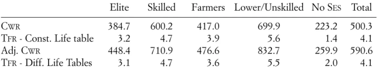
Figure 2 shows estimates of CWRand OCMby socioeconomic status for Sweden
around 1900. Since occupational status could vary over time, the average fertility levels by socioeconomic status have been summarized only for the five year period before the census (1896-1900). As expected, the total fertility rates varied with socioeconomic status. The elite groups had the lowest fertility rates, confirming its role as the forerunner in the decline of fertility.
Even if migration movements could affect these measures, it is sensible to assume that mothers generally move together with their children. In this case, migration should be scarcely able to alter these indirect estimates of fertility (De Santis 2003). However, these CWR and OCM estimates do not take into account
socioeconomic differences in mortality, since no national level information about mor-tality risks by socioeconomic status are available for that time. Socioeconomic differ-ences in mortality should have a relatively limited impact on these estimates, however, because mortality was quite similar across socioeconomic groups before the demo-graphic transition (Knodel 1983; Surault 1979; Smith 1983). Nonetheless, at the begin-ning of the demographic transition, the upper classes might have been the first to take advantage of improved hygiene and sanitation as well as of better nutrition, and there-fore experienced mortality decline earlier than other social groups (Marmot 2004). While there is some empirical support for this hypothesis for infant and child mortal-ity in Sweden (Bengtsson, Dribe 2010) it is not the case for adult mortalmortal-ity where pro-nounced socioeconomic differences in mortality did not emerge until after World War II (Bengtsson, Dribe 2011; Edvinsson, Lindkvist 2011).
OCM estimates will underestimate fertility levels for high mortality groups in
rela-tion to low mortality groups. To assess the importance of this potential bias we have looked at Malmöhus county in southern Sweden and used age-specific mortality rates by socioeconomic status available from the Scanian Economic Demographic Database3 (Bengtsson, Dribe 2011) to adjust the CWR estimates for mortality and
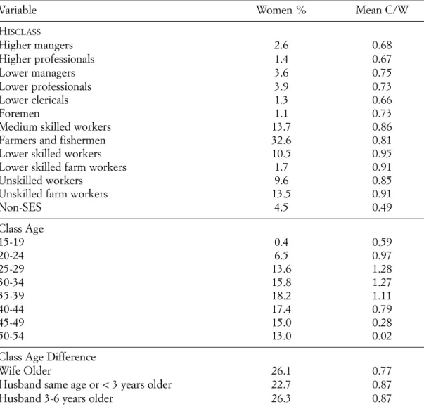
then compare to the unadjusted estimates (see Dribe, Scalone forthcoming). The adjustments correct for both infant mortality and adult mortality in reproductive ages. The full set of estimates is shown in Table 1. The first OCM estimate of TFR
assumes the average mortality risks by age for all social groups, whereas the second 0,0 100,0 200,0 300,0 400,0 500,0 600,0 700,0 800,0 0,0 1000,0 2000,0 3000,0 4000,0 5000,0 6000,0 7000,0 Higher managers Higher Lower managers
Lower professional Lower clericals Foremen Mediu m skil led Farmers Lowe r skil led Lowe r skil led fa rm Unskilled workers Un skille d farm TFR based on OCM unadj. CWR To ta l F er til ity R at e * 1000 C hi ld -W om an R at io * 1000 Figure 3a
Fig. 2. Child-woman ratio and own-children estimates of total fertility rates in Sweden (1896-1900)
Source: our own computation on Swedish Census of 1900 Data from North Atlantic Population Project Database – Swedish National Archive and Human Mortality Database.
Note: Women without socio-economic status and domestic servants have been excluded.
Tab. 1. Child-Woman Ratios and Total Fertility Rates by Socio-Economic Status, Malmöhus
(1896-1900)
Elite Skilled Farmers Lower/Unskilled No SES Total
CWR 384.7 600.2 417.0 699.9 223.2 500.3
TFR- Const. Life table 3.2 4.7 3.9 5.6 1.4 4.1
Adj. CWR 448.4 710.9 476.6 832.7 259.9 590.6
TFR- Diff. Life Tables 3.1 4.7 3.6 5.5 2.0 4.1 Source: Our own computation on Swedish Census of 1900 Data from North Atlantic Population Project Database – Swedish National Archive and Scanian Demographic Database.
Note: Elite = Managers, professionals, clericals, sales’ personnel and foremen (1-6); Skilled = Middle skilled and Lower skilled workers (7 and 9); Farmers = Farmers and Fishermen (8); Lower/Unskilled = Lower farm workers, Unskilled farm and non-farm Workers (10-11-12).
Highe r profe
ssiona ls
one uses specific life tables for each socioeconomic group. With the possible excep-tion of farmers, the two estimates of total fertility are broadly similar and even in the case of farmers the difference is only about eight percent.
For CWR the differences between the estimates is greater than for TFR.
Calculating unadjusted CWR, no corrections for mortality have been made,
where-as in our first OCM application, at least the adopted constant life table takes into
account the average mortality level. However it is important to note that the rela-tive positions of the different socioeconomic groups are the same in both estimates. Hence, even though the magnitudes of the estimates differ somewhat, this exercise shows that unadjusted CWRs give a fairly good picture of fertility differentials by
socioeconomic status. It is also important to remember that, to the extent that high status groups had lower CWR than low status groups in the transition in Sweden,
this was not likely an effect of higher mortality in these groups as we would, if any-thing, expect the upper classes to have gained an advantage in infant and child sur-vival. In other words, it may well be the case that true fertility differentials are underestimated rather than overestimated when using CWR. Moreover, regardless
of this bias, the unadjusted CWRwill serve as a useful indicator of net fertility, which
after all is what is most relevant in the fertility transition. In the following analysis this is also how we will interpret the main results, that is, as indicators of net fertil-ity rather than gross fertilfertil-ity.
5. Determinants of net fertility. The descriptive measures presented in the previ-ous section showed the basic socioeconomic differences in net fertility. However, when fertility of different groups is compared, the CWRcould also be affected by
variations in the proportion of married women. In addition, fertility decline in Sweden, as in other parts of Europe, can mainly be attributed to a decline in mari-tal fertility rather than changes in nuptiality (Dribe 2009). For this reason the analy-sis in the rest of the paper will focus on marital fertility taking into account only ever married women living with their own husband.
We estimate the association between socioeconomic status and net fertility using regression models. The idea is to control for a number of possible explanatory variables and spatial heterogeneity in estimating the association. The main covariate is the socioe-conomic status of the husband, based on the declared occupations in the census.
To account for other factors correlated with both socioeconomic status and net fer-tility, we also control for variables at the individual, household and parish levels. At the onset of the fertility transition, some individual demographic characteristics, such the age of the woman and her husband, still played an important role. On the one hand women in peak reproductive ages had more children, but on the other hand couples in which husbands were much older than their wives had lower fertility.
Since migration may also reduce marital fertility by a sense of precariousness which can affect immigrants, a categorical variable for migrant status is also includ-ed in the analysis. Moreover, given that in traditional societies childrearing has always been a female task, women’s labor force participation4meant greater
diffi-culties in looking after small children. In addition, female labor force participation promoted the material aspirations of women and changes in gender roles which may particularly have affected the fertility of high status groups (Brown, Guinnane 2002; Caldwell 1999).
Turning to the household structure, we also control for whether or not the hus-band was the head of household, expecting non-heads to have lower fertility. In addition, because older women (more than 54 years of age) or servants in the house-hold could have provided assistance in child care, and thereby limiting the oppor-tunity cost of children, two additional dummy variables have been included.
At a geographical level, the diffusion of new attitudes about birth control and the ideal family size was based on a macro process of social modernization, sub-stantially based on industrialization, migration, urbanization, education and female work. In addition, all these components were strongly correlated with economic and social changes that contributed to reduce the benefits of children and increase their costs (Dribe 2009). Therefore the analysis takes into account four additional macro indicators that have been calculated at parish level: the proportion of migrants in the total population, the number of teachers in basic education per 100 children in school age 7-14, the number of women who participate in the labor force relative to the female population aged 15-64, the number of workers in indus-tries and manufactories (major groups 7/8/9 of HISCO code) relative to the male
population aged 15-64. Finally a control for urban residence is also included. 6. Method. Ordinary least squares regression (OLS) models have been estimated to
assess the association between socioeconomic status and the number of children under 5 for each married woman aged 15-54. In total, the analysis takes into account 621,397 married women living with their husbands and 512,082 own chil-dren. We also consider the influence of the geographical context by estimating a parish-level fixed-effects model (FE).
The OLSmodel is formulated as:
(1)
where the dependent variable Y is the number of own children under 5 of a mar-ried women i that lives in parish j. SES represents a categorical variable for
socio-economic status, X is a sets of dummy covariates for each individual (age, age dif-ferences between spouses, migrant status and female work) and household charac-teristics (household head, other older women and servants in the same dwelling). Z is a set of community level indicators (industrial, migrant, education and female labor force participation rates) related to parish j and U is a dichotomous control for urban or rural area.
The FEmodel can be written as:
where υjis the parish-specific residual and εijis the individual woman’s residual. The fixed-effects specification implies that the group-specific heterogeneity is assumed to be constant, and thus controls for invariant differences between groups (parishes in this case) that are not captured in the previous OLSmodel.
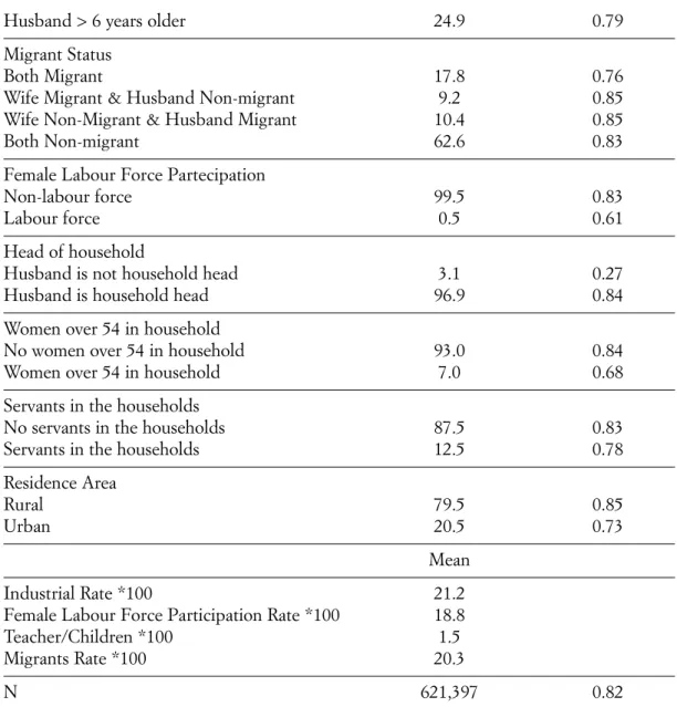
7. Empirical results. Before turning to the results, it is worth looking at the descrip-tive statistics. Table 2 displays the percentage distribution of married women aged 15-54 and the mean number of children under 5 for each of the variables. Because agriculture was still the predominant activity in Sweden at the end of the nineteenth century, 47.8% of the women were married to a husband who worked in agricul-ture. Actually the most frequent occupational statuses were farmers (32.6%) and unskilled farmer workers (13.5%). Lower farmers (1.7%) were evidently less fre-quent. Medium skilled workers (13.7%) and lower skilled workers (10.5%) were predominant among the urban social groups, since the upper social categories (from foremen to higher managers) totally grouped 13.9% of the women.
Tab. 2. Descriptive statistics
Variable Women % Mean C/W
HISCLASS Higher mangers 2.6 0.68 Higher professionals 1.4 0.67 Lower managers 3.6 0.75 Lower professionals 3.9 0.73 Lower clericals 1.3 0.66 Foremen 1.1 0.73
Medium skilled workers 13.7 0.86 Farmers and fishermen 32.6 0.81 Lower skilled workers 10.5 0.95 Lower skilled farm workers 1.7 0.91 Unskilled workers 9.6 0.85 Unskilled farm workers 13.5 0.91
Non-SES 4.5 0.49 Class Age 15-19 0.4 0.59 20-24 6.5 0.97 25-29 13.6 1.28 30-34 15.8 1.27 35-39 18.2 1.11 40-44 17.4 0.79 45-49 15.0 0.28 50-54 13.0 0.02
Class Age Difference
Wife Older 26.1 0.77
Husband same age or < 3 years older 22.7 0.87 Husband 3-6 years older 26.3 0.87
It is interesting to note that the upper classes had systematically lower CWRthan
the other social groups. This pattern of net fertility by SESis almost identical to TFR
and CWRthat we already presented in the previous section (there are some minor
differences because here we are considering marital fertility and not total fertility). In fact, since the mean number of children has been calculated by simply dividing the number of children by the number of married women, these averages could be interpreted as marital CWRs. For instance, we can say that there were on average 810
children under 5 per 1000 women married to farmers. Moreover, we can easily extend this interpretation to the parameters of the regression models that we have just defined, by reading them as the estimated covariate effects on the marital CWR.
Table 3 shows estimations of OLS and FEmodels. Starting from a basic model
Husband > 6 years older 24.9 0.79 Migrant Status
Both Migrant 17.8 0.76
Wife Migrant & Husband Non-migrant 9.2 0.85 Wife Non-Migrant & Husband Migrant 10.4 0.85 Both Non-migrant 62.6 0.83 Female Labour Force Partecipation
Non-labour force 99.5 0.83
Labour force 0.5 0.61
Head of household
Husband is not household head 3.1 0.27 Husband is household head 96.9 0.84 Women over 54 in household
No women over 54 in household 93.0 0.84 Women over 54 in household 7.0 0.68 Servants in the households
No servants in the households 87.5 0.83 Servants in the households 12.5 0.78 Residence Area
Rural 79.5 0.85
Urban 20.5 0.73
Mean Industrial Rate *100 21.2 Female Labour Force Participation Rate *100 18.8 Teacher/Children *100 1.5 Migrants Rate *100 20.3
N 621,397 0.82
Source: Our own computation on Swedish Census of 1900 from North Atlantic Population Project Database – Swedish National Archive.
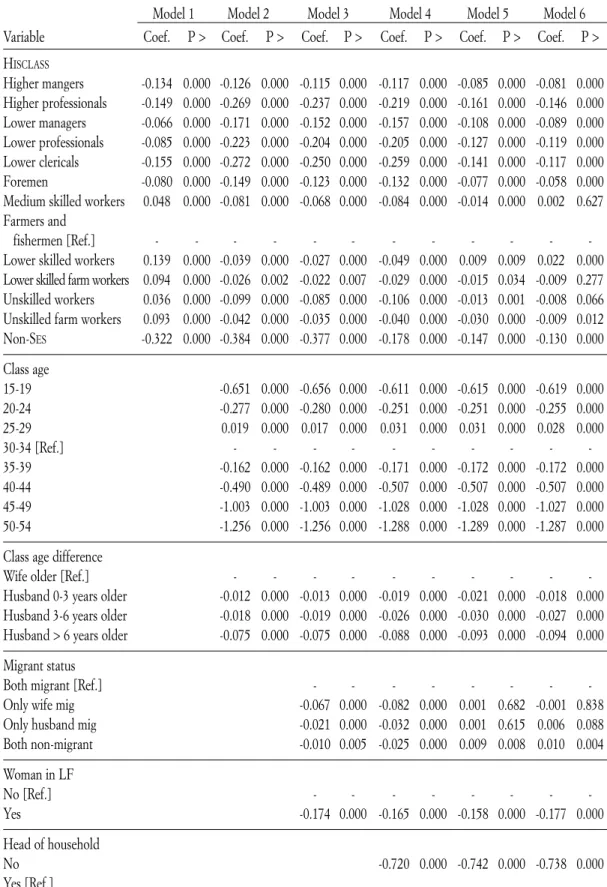
Tab. 3. Regression model estimates for the number of children 0-4 per married women 15-54
aged (C/W), Sweden (1900)
Model 1 Model 2 Model 3 Model 4 Model 5 Model 6 Variable Coef. P > Coef. P > Coef. P > Coef. P > Coef. P > Coef. P > HISCLASS Higher mangers -0.134 0.000 -0.126 0.000 -0.115 0.000 -0.117 0.000 -0.085 0.000 -0.081 0.000 Higher professionals -0.149 0.000 -0.269 0.000 -0.237 0.000 -0.219 0.000 -0.161 0.000 -0.146 0.000 Lower managers -0.066 0.000 -0.171 0.000 -0.152 0.000 -0.157 0.000 -0.108 0.000 -0.089 0.000 Lower professionals -0.085 0.000 -0.223 0.000 -0.204 0.000 -0.205 0.000 -0.127 0.000 -0.119 0.000 Lower clericals -0.155 0.000 -0.272 0.000 -0.250 0.000 -0.259 0.000 -0.141 0.000 -0.117 0.000 Foremen -0.080 0.000 -0.149 0.000 -0.123 0.000 -0.132 0.000 -0.077 0.000 -0.058 0.000 Medium skilled workers 0.048 0.000 -0.081 0.000 -0.068 0.000 -0.084 0.000 -0.014 0.000 0.002 0.627 Farmers and
fishermen [Ref.] - - -
-Lower skilled workers 0.139 0.000 -0.039 0.000 -0.027 0.000 -0.049 0.000 0.009 0.009 0.022 0.000 Lower skilled farm workers 0.094 0.000 -0.026 0.002 -0.022 0.007 -0.029 0.000 -0.015 0.034 -0.009 0.277 Unskilled workers 0.036 0.000 -0.099 0.000 -0.085 0.000 -0.106 0.000 -0.013 0.001 -0.008 0.066 Unskilled farm workers 0.093 0.000 -0.042 0.000 -0.035 0.000 -0.040 0.000 -0.030 0.000 -0.009 0.012 Non-SES -0.322 0.000 -0.384 0.000 -0.377 0.000 -0.178 0.000 -0.147 0.000 -0.130 0.000 Class age 15-19 -0.651 0.000 -0.656 0.000 -0.611 0.000 -0.615 0.000 -0.619 0.000 20-24 -0.277 0.000 -0.280 0.000 -0.251 0.000 -0.251 0.000 -0.255 0.000 25-29 0.019 0.000 0.017 0.000 0.031 0.000 0.031 0.000 0.028 0.000 30-34 [Ref.] - - - -35-39 -0.162 0.000 -0.162 0.000 -0.171 0.000 -0.172 0.000 -0.172 0.000 40-44 -0.490 0.000 -0.489 0.000 -0.507 0.000 -0.507 0.000 -0.507 0.000 45-49 -1.003 0.000 -1.003 0.000 -1.028 0.000 -1.028 0.000 -1.027 0.000 50-54 -1.256 0.000 -1.256 0.000 -1.288 0.000 -1.289 0.000 -1.287 0.000 Class age difference
Wife older [Ref.] - - -
-Husband 0-3 years older -0.012 0.000 -0.013 0.000 -0.019 0.000 -0.021 0.000 -0.018 0.000 Husband 3-6 years older -0.018 0.000 -0.019 0.000 -0.026 0.000 -0.030 0.000 -0.027 0.000 Husband > 6 years older -0.075 0.000 -0.075 0.000 -0.088 0.000 -0.093 0.000 -0.094 0.000 Migrant status
Both migrant [Ref.] - - -
-Only wife mig -0.067 0.000 -0.082 0.000 0.001 0.682 -0.001 0.838
Only husband mig -0.021 0.000 -0.032 0.000 0.001 0.615 0.006 0.088
Both non-migrant -0.010 0.005 -0.025 0.000 0.009 0.008 0.010 0.004 Woman in LF No [Ref.] - - - -Yes -0.174 0.000 -0.165 0.000 -0.158 0.000 -0.177 0.000 Head of household No -0.720 0.000 -0.742 0.000 -0.738 0.000 Yes [Ref.]
(1) that takes into account only socioeconomic status, control variables for demo-graphic and other characteristics of the woman (2 and 3) and the household (4) have been progressively included. At geographical level, model 5 estimates the effects of four parish indicators, whereas model 6 controls for unobserved spatial heterogeneity by directly including fixed-effects (FE) at parish level.
Looking first at Model 1 there is a clear association between socioeconomic sta-tus and CWR, with the working classes having more children than the higher status
groups. More specifically, the estimated coefficients range from -0.155 for lower clericals to +0.129 for lower skilled workers. As the average CWRfor farmers (the
reference category) is 820 children per 1000 women, lower clerical and lower skilled workers have -155 and +129 children respectively, which is equivalent to 19% less and 17% more children, respectively.
Obviously these are the same figures already reported in Table 2. When adding controls for age of woman and her spouse (model 2), farmers show the highest CWR
and coefficients for the upper classes (from higher managers to foremen) are much lower, while the lower classes fall in-between. Evidently, part of the gross socioeco-nomic differences in fertility is explained by different age distributions, which of course has a big impact on fertility. According to the parameters in model 2, farmer women in the reference category (age group 30-34 and older than their husbands) had 1.37 children, whereas an identical woman married to a lower clerical husband had 1.10 (-0.272+1.373), in other words about 20% fewer children. Similarly, high-er professionals, lowhigh-er professionals and lowhigh-er managhigh-ers had, respectively, 19.5,
Women over 54 in household
No [Ref.] - - -
-Yes -0.079 0.000 -0.081 0.000 -0.065 0.000
Servants in the households
No [Ref.] - - - -Yes -0.050 0.000 -0.026 0.000 -0.015 0.000 Residence area Rural [Ref.] - -Urban -0.075 0.000 Industrial rate *100 -0.001 0.000 FLFP*100 -0.003 0.000 Teacher/Children *100 -0.017 0.000 Migrants Rate *100 -0.002 0.000 Const 0.814 0.000 1.373 0.000 1.380 0.000 1.434 0.000 1.532 0.000 1.363 0.000 Fixed effects Sigma_u 0.131 Sigma_e 0.786 Rho 0.027
Source: Our own computation on Swedish Census of 1900 from North Atlantic Population Project Database – Swedish National Archive.
16.5 and 12.4% fewer children than farmers. Lower skilled farm workers and lower skilled workers had much the same CWRas farmers: 1.9 and 2.8% less,
respective-ly. Non-farm workers had 7.2% fewer children and the corresponding figure for unskilled farm workers was 3.0%.
Moreover, these observed socioeconomic differentials in CWRdo not vary when
controls for migrant status, female employment (model 3) and household structure (model 4) are taken into account. According to these results, farmers and workers in agriculture still had a higher fertility than the other groups, which may well have been related to a higher demand for children in more traditional agrarian settings, because of the lower costs and the higher benefits of children.
Quite unexpectedly, the presence of older women and servants in the household were both associated with lower CWR. Rather than suggesting a lack of
intergener-ational solidarity, this should probably be interpreted as an effect of the limited resources in the domestic aggregated when the number of members increases.
In model 5, the degree of industrialization, female labor force participation, pro-portion of migrants and number of teachers per school children at the community level all showed negative associations with CWR. As expected, urban areas also had
lower average CWR than rural areas. More interestingly, however, controlling for
socioeconomic characteristics of the parish further reduced the socioeconomic dif-ferentials. For instance, the coefficients of lower clericals decrease from -0.272 to -0.141, whereas the effects of unskilled workers reduced from -0.099 to -0.013. According to model 2, lower clericals had 24.8% lower CWR than farmers, but
according to model 5, this difference was only 10.1% for a woman in the reference category. Similarly, unskilled workers had 7.8% lower CWRthan farmers according
to model 2 but only 0.9% less according to model 5.
Estimating a parish-level fixed effects model lowers the socioeconomic differ-entials even further (model 6). Comparing the effects for the higher social groups in model 2 and 6, almost all coefficients were reduced by about a half. In addition, parameter estimates for medium skilled workers, lower skilled farm workers and unskilled workers approached zero, indicating very similar CWRs as farmers. It is
interesting to note that, since age is a physiological determinant, its effect did not vary when spatial and geographical heterogeneity was taken into account.
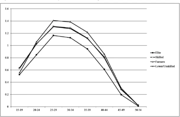
In order to show even more clearly that the association between socioeconomic status and a decline in CWR when taking geographical and contextual differences
into account, we calculated the predicted number of children per married woman (marital CWR) by socioeconomic status and age of the mother for women in the
ref-erence categories. Figure 3 displays these predicted values based on model 2 (only age controls) and model 6 (full model with FE) respectively.
Comparing Figure 3a and 3b reveals immediately the smaller socioeconomic dif-ferentials in the full models compared to the model where only age is controlled for. This clearly shows the importance of spatial patterns for the socioeconomic differ-entials at the national level. At least half the variation across socioeconomic groups was explained by spatial heterogeneity. Nonetheless, in a model controlling for a number of individual, family and community characteristics as well as unobserved
Fig. 3a. Predicted C/W ratio by SESand mother’s age class based on model 2
Note: Elite = Managers, professionals, clericals, sales´ personnel and foremen (1-6); Skilled = Middle skilled and Lower skilled workers (7 and 9); Farmers = Farmers and Fishermen (8); Lower/Unskilled = Lower farm workers, Unskilled farm and non-farm workers (10-12).
parish level heterogeneity, the elite groups (HC 1-6) had lower fertility than the
other groups in 1900, i.e. about 15-20 years into the fertility transition.
8. Conclusion. In this paper, we have analyzed socioeconomic differential in net fertility in Sweden at the end of the nineteenth century. Since official sources do not provide vital statistics by socioeconomic status, we based our analysis on Swedish census data of 1900, employing indirect techniques of fertility estimation. The child-woman ratio used in the main analysis was not adjusted for mortality but instead served as an indicator of net fertility. We could however, also demonstrate that these unadjusted CWRs did a reasonably good job also in indicating
socioeco-nomic differentials in gross, or total, fertility. The fact that socioecosocioeco-nomic differ-ences in mortality overall appear to have been quite limited before and during the demographic transition supports this view.
In the introductory section we reviewed some previous research and some the-oretical underpinnings of fertility differentials during the fertility transitions. Based on this discussion, we hypothesized that higher social status should have been asso-ciated with relatively low fertility during the transition because higher status groups acted as forerunners in the decline. Our results also supported this hypothesis.
The crude socioeconomic differentials in net fertility were substantial in Sweden immediately before 1900, with elite groups having considerably lower marital child-woman ratios than the working classes. However, these crude differences were part-ly explained by compositional differences between classes according to age, com-munity context and spatial heterogeneity. When we controlled for these factors socioeconomic differentials in net fertility declined substantially, but did not vanish completely. Even when we controlled for individual and household variables as well as parish level fixed effects, the elite group and the upper middle class had consid-erably lower net fertility than the other groups.
The lower fertility of the higher status groups can partly be explained by an adjustment to new conditions following increased returns to education and other impacts of modernization on costs and benefits of children. Female labor force participation, urban residence, more industrial employment, and higher com-munity investments in education all show the expected signs and thus con-tribute to explain lower fertility. More importantly, including these controls lowered the socioeconomic differentials, which indicate that at least part of the explanation for the negative association between socioeconomic status and fer-tility was an adjustment to new conditions, and this adjustment came earlier and stronger in the higher classes.
However, the fact that the socioeconomic differentials were clearly visible also when having controlled for many of the adjustment variables point to the possibil-ity that innovation processes were also at work. As discussed in the theoretical sec-tion, the elite and the higher social groups were better able to acquire new knowl-edge and information and may also have been more open to new ideas, and chang-ing attitudes than lower classes. In other words, the elite groups were forerunners not only in terms of fertility decline but also in modernization more generally (Frykman, Löfgren 1978).
Finally, it deserves to be mentioned once again that this has only been a prelim-inary study taking a first look at the census evidence for one single year. In the near future we will expand the analysis by including the censuses of 1890 and 1880 which will enable not only a more detailed picture of the early movers in the fertil-ity decline to emerge, but will also allow us to study the dynamics of this process through using linked data where we can follow families in two or even three cen-suses.
1It is possible to find full information, complete documentation and data at the NAPP website: http://www.nappdata.org/napp/index.shtml 2 At the website of the History Of Work Information System, it is possible to find doc-umentation, bibliography and information on the historical international classification of occupations (HISCO) and the on the social class scheme HISCLASS: http://historyofwork.iisg.nl/ index.php. The classification into HISCLASS
was made using the recode job: [email protected], May 2004, see http://history- ofwork.iisg.nl/list_pub.php?categories=his-class
3It possible to find further information on the Scanian Demographic Database (SDD) at the fol-lowing web address: http://www.ed.lu.se/EN/ databases/sdd.asp.
4 Since the census data register a suspiciously low number of women in labour force, we pre-fer to view this covariate as a gross indicator.
References
Minnesota Population Center. North Atlantic Population Project: Complete Count Microdata. Version 2.0 [Machine-readable database]. Minneapolis: Minnesota Popu-lation Center, 2008.
The Swedish National Archives, Umeå University, and the Minnesota Population Center. National Sample of the 1900 Census of Sweden, Version 1.0. Minneapolis: Minnesota Population Center [distributor], 2008.
G.S. Becker 1991, A Treatise on the Family, Harvard University Press, Cambridge, MA. S.O. Becker, F. Cinnirella, L. Woessmann
2010, The trade-off between fertility and
edu-cation: evidence from before the demographic transition, «Journal of Economic Growth»,
15, 177-204.
T. Bengtsson, M. Dribe 2006, Deliberate
con-trol in a natural fertility population: Southern Sweden 1766-1865, «Demography», 43,
727-746.
T. Bengtsson, M. Dribe 2011, The late
emer-gence of socioeconomic mortality differen-tials: A micro-level study of adult mortality in
southern Sweden 1815-1968, «Explorations
in Economic History», 48, 389-400.
N. Boberg-Fazlic, P. Sharp, J. Weisdorf 2011,
Survival of the richest? Social status, fertility and social mobility in England 1541-1824,
«European Review of Economic History», 15, 365-392.
H. Bras, J. Kok, K. Mandemakers 2010,
Sibship size and status attainment across con-texts: Evidence from the Netherlands, 1840-1925, «Demographic Research», 23, 73-104.
J.C. Brown, T.W. Guinnane 2002, Fertility
transition in a rural, Catholic population: Bavaria, 1880-1910, «Population Studies»,
56, 35-50.
J. Caldwell 1999, The delayed western fertility
decline: An examination of English speaking Countries, «Population and Development
Review», 25, 3, 479-513.
G. Carlsson 1966, The decline of fertility:
inno-vation or adjustment process, «Population
Studies», 20, 149-174.
L.J. Cho, R.D. Retherford, M.K. Choe 1986,
The Own-Children Method of Fertility Estimation, Honolulu, University of Hawaii
Press.
Economic History of the World, Princeton,
Princeton University Press.
G. Clark, N. Cummins 2009, Urbanization,
mortality, and fertility in Malthusian En-gland, «American Economic Review: Papers
& Proceedings», 99, 242-247.
G. Clark, G. Hamilton 2006, Survival of the
richest: the Malthusian mechanism in pre-industrial England, «Journal of Economic
History», 66, 707-736.
J.R. Cleland, C. Wilson 1987, Demand theories
of the fertility transition: An iconoclastic view, «Population Studies», 41, 5-30.
J. Cleland 2001, Potatoes and pills: An
overview of innovation-diffusion contribu-tions to explanacontribu-tions of fertility decline, in J.
Casterline (ed.), Diffusion Processes and
Fertility Transition: Selected Perspectives,
Washington, D.C., National Research Council, 39-65.
A.J. Coale 1973, The demographic transition
reconsidered. International Population Conference, 1, Liège, International Union
for the Scientific Study of Population. A.J. Coale, S.C. Watkins (eds.) 1986, The
Decline of Fertility in Europe, Princeton,
Princeton University Press.
N.F.R. Crafts 1984, A time series study of
fertil-ity in England and Wales, 1877-1938,
«Journal of European Economic History», 13, 571-590.
N. Cummins 2009, Marital fertility and wealth
in transition era France, 1750-1850, Working
paper-Paris School of Economics, 16. P.A. David, W.C. Sanderson 1986,
Ru-dimentary contraceptive methods and the American transition to marital fertility con-trol, 1855-1915, in S.L. Engerman, R.E.
Gallman (eds.), Long-Term Factors in
American Economic Growth, Chicago, The
University of Chicago Press.
G. De Santis 2003, The own-children method of
fertility estimation in historical demography: a glance backward and a step forward, in M.
Breschi, S. Kurosu, M. Oris (eds.), The
Own-Children Method of Fertility Esti-mation: Applications in Historical Demo-graphy, Udine, Forum.
M. Doepke 2005, Child mortality and fertility
decline: Does the Barro-Becker model fit the facts?, «Journal of Population Economics»,
18, 337-366.
M. Dribe 2009, Demand and supply factors in
the fertility transition: a county-level analysis of age-specific marital fertility in Sweden, 1880-1930, «European Review of Economic
History», 13, 65-94.
M. Dribe, F. Scalone 2010, Detecting
Deliberate Fertility Control in Pre-transition-al Populations: Evidence from six German villages, 1766-1863, «European Journal of
Population», 26, 411-434.
M. Dribe, F. Scalone (forthcoming), Measuring
socio-economic differences in fertility by using NAPP data: Tests on the Swedish Census of
1900.
R.A. Easterlin, E.C. Crimmins 1985, The
Fertility Revolution: A Supply-Demand Analysis, Chicago, University of Chicago
Press.
K.A. Edin, E.P. Hutchinson 1935, Studies of
Differential Fertility in Sweden, London, P.S.
King & Sons.
S. Edvinsson, M. Lindkvist 2011, Wealth and
health in 19th century Sweden. A study of social differences in adult mortality in the Sundsvall region, «Explorations in
Eco-nomic History», 48, 376-388.
J. Frykman, O. Löfgren 1987, Culture
Buil-ders: A Historical Anthropology of Middle-Class Life, New Brunswick, Rutgers
University Press.
P.R. Galloway, E.A. Hammel, R.D. Lee 1994,
Fertility decline in Prussia, 1875-1910: a pooled cross-section time series analysis,
«Population Studies», 48, 135-181.
P.R. Galloway, R.D. Lee, E.A. Hammel 1998,
Infant mortality and the fertility transition: Macro evidence from Europe and new find-ings from Prussia, in M.R. Montgomery, B.
Cohen (eds.), From Death to Birth: Mortality
and Reproductive Change, Washington D.C.,
National Research Council.
O. Galor 2005, From Stagnation to Growth:
Unified Growth Theory, in P. Aghion, S.N.
Durlauf (eds.), Handbook of Economic
Growth, 1A, Amsterdam, Elsevier.
E. Garrett, A. Reid, K. Schürer, S. Szreter 2001, Changing Family Size in England and
Wales. Place, Class and Demography, 1891-1911, Cambridge, Cambridge University
Press.
M.R. Haines 1992, Occupation and social class
during fertility decline: historical perspectives,
in J.R. Gillis, L.A. Tilly, D. Levine (eds.),
The European Experience of Changing Fertility, Cambridge, MA, Blackwell.
L. Henry 1961, Some data on natural fertility, «Eugenics Quarterly», 8, 81-91.
R. Lesthaeghe, C. Vanderhoeft 2001, Ready,
willing, and able: A conceptualization of tran-sitions to new behavioral forms, in J.
Fertility Transition: Selected Perspectives,
Washington, D.C., National Research Council, 240-264.
J. Knodel 1983, Seasonal Variation in Infant
Mortality: An Approach with Applications,
«Annales de Démographie Historique», 23-35, 1983.
J. Knodel, E. van de Walle 1979, Lessons from
the past: Policy implications of historical fer-tility studies, «Population and Development
Review», 5, 117-145.
M. Livi-Bacci 1986, Social-group forerunners of
fertility control in Europe, in A.J. Coale, S.C.
Watkins (eds.), The Decline of Fertility in
Europe, Princeton, Princeton University
Press.
M. Marmot 2004, Status Syndrome. How Your
Social Standing Directly Affects Your Health and Life Expectancy, London, Bloomsbury
Publishing.
C. Mosk 1983, Patriarchy and Fertility: Japan
and Sweden, 1880-1960, New York,
Aca-demic Press.
D. Reher 1999, Back to the basics: Mortality
and fertility interactions during the demo-graphic transition, «Continuity and
Chan-ge», 14, 9-31.
D.S. Reher, A. Sanz-Gimeno 2007, Rethinking
historical reproductive change: Insights from longitudinal data for a Spanish town,
«Po-pulation and Development Review», 33, 703-727.
S. Ruggles, E. Roberts, S. Sarkar, M. Sobek 2011, The North Atlantic Population
Project: Progress and Prospects, «Historical
Methods: A Journal of Quantitative and Inter-disciplinary History», 44, 1, 1-6.
G. Santow 1995, Coitus interruptus and the
control of natural fertility, «Population
Studies», 49, 19-43.
J.C. Schneider, P.T. Schneider 1996, Festival of
the Poor. Fertility Decline and the Ideology of Class in Sicily 1860-1980, Tucson, AZ, The University of Arizona Press.
T.P. Schultz 1985, Changing world prices,
women’s wages, and the fertility transition, Sweden, 1860-1910, «Journal of Political
Economy», 93, 1126-54.
V. Skirbekk 2008, Fertility trends by social status, «Demographic Research», 18, 5, 145-180. D.S. Smith 1983, Differential Mortality in the
United States before 1900, «Journal of
Interdisciplinary History», 13, 735-759. M. Sobek, L. Cleveland, S. Flood, P.K. Hall,
M.L. King, S. Ruggles, M. Schroeder 2011,
Big Data: Large-Scale Historical Infrastructure from the Minnesota Population Center,
«Hi-storical Methods: A Journal of Quantitative and Interdisciplinary History», 44, 2, 61-68. S. Sogner, H.B. Randsborg, E. Fure 1984, Fra
stua full til tobarnskull, Universitetsforlaget,
Oslo.
H.S. Shryock, J.S. Siegel 1980, The Methods
and Materials of Demography, Washington
D.C., Bureau of the Census.
S. Szreter 1996, Fertility, Class and Gender in
Britain 1860-1940, Cambridge, Cambridge
University Press.
P. Surault 1979, L’Inégalité devant la mort, Paris, Economica.
UN 1983, Manual X. Indirect Techniques for
Demographic Estimation, United Nation,
New York.
J. Van Bavel 2004, Deliberate birth spacing
before the fertility transition in Europe. Evidence from nineteenth-century Belgium,
«Population Studies», 58: 95-107.
J. Van Bavel 2006, The effect of fertility
limita-tion on intergeneralimita-tional social mobility: The quantity-quality trade-off during the demo-graphic transition, «Journal of Biosocial
Science», 38, 553-569.
J. Van Bavel, S. Moreels, B. Van de Putte, K. Matthijs 2011, Family size and
intergenera-tional social mobility during the fertility tran-sition: Evidence of resource dilution from the city of Antwerp in nineteenth century Belgium,
«Demographic Research», 24, 313-344. B. Van de Putte 2007, The influence of modern
city life on marriage in Ghent at the turn of the twentieth century: Cultural struggle and social differentiation in demographic behavior,
«Journal of Family History», 32, 433-458. M.H.D. Van Leeuwen, I. Maas 2010, Historical
studies of social mobility and stratification,
«Annual Review of Sociology», 36, 429-451. M.H.D. Van Leeuwen, I. Maas 2011, HISCLASS.
A Historical International Social Class Scheme, Leuven, Leuven University Press.
M.H.D. Van Leeuwen, I. Maas, A. Miles 2002,
HISCO. Historical International Standard
Classification of Occupations, Leuven,
Leuven University Press.
J.B. Wahl 1992, Trading quantity for quality.
Explaining the decline in American fertility in the nineteenth century, in C. Goldin, H.
Rockoff (eds.), Strategic Factors in
Nine-teenth Century American Economic History. A Volume to Honor Robert W. Fogel,
Summary
Socioeconomic status and net fertility in the demographic transition: Sweden in 1900 – A preliminary analysis
There has recently been a renewed interest in the socioeconomic aspects of reproduction during the great fertility decline. While most previous work on the European fertility decline has been macro-oriented, using various kinds of aggregate data picturing of the demographic processes at regional or national level, much less has been done using micro-level data, and specifically look-ing at patterns across social groups. In this paper we look at the association between socioeco-nomic status and net fertility in Sweden’s fertility transition using micro-level census data cover-ing the entire population around 1900. The data contain information on number of children by age, occupation of the mother and father, place of residence and household context. Coding occu-pations in HISCOand classifying them into a social class scheme (HISCLASS) enables us to study the impact of socioeconomic status on number of children under 5, controlling also for spatial varia-tions in social stratification. Our results indicate that the crude socioeconomic differentials in net fertility were substantial in Sweden immediately before 1900, with the elite and the upper middle classes having considerably lower marital child-woman ratios than the working classes. However, these crude differences were partly explained by compositional differences between classes according to age, community context and spatial heterogeneity. Nonetheless, even when control-ling for individual and household variables as well as parish level fixed effects, the elite group had considerably lower net fertility than the other groups.
Riassunto
Stato socioeconomico e fecondità netta durante la transizione demografica: la Svezia nel 1900 – Un’analisi preliminare
Recentemente vi è stato un rinnovato interesse per gli aspetti socioeconomici del comportamento riproduttivo durante la grande transizione della fecondità. Mentre gran parte delle ricerche pre-cedenti sul declino della fecondità in Europa sono state sviluppate in termini macro, sfruttando dati aggregati e dando un quadro dei processi demografici e delle determinanti economiche a livel-lo regionale e nazionale, molto meno è stato fatto sulla base di dati micro, e specificamente per prendere in considerazione l’emergere delle differenziazioni tra gruppi sociali. In questo articolo, abbiamo studiato l’associazione tra stato socioeconomico e fecondità netta durante la transizione della fecondità in Svezia, utilizzando dati censuari a livello micro e considerando l’intera popola-zione poco prima del 1900. I dati forniscono informazioni riguardo al numero di figli, all’occupa-zione del padre e della madre, e al contesto familiare. La codifica HISCOdelle occupazioni e la riag-gregazione di queste nello schema di classificazione sociale HISCLASSci ha permesso di studiare l’impatto dello stato socioeconomico sul numero dei figli sotto i cinque anni di età, tenendo sotto controllo gli effetti dovuti alle variazioni spaziali della stratificazione sociale. I nostri risultati mostrano come le differenze socioeconomiche in termini di fecondità netta erano ben evidenti in Svezia già poco prima del 1900, con i marital child-woman ratios delle élite e delle classi medio-alte considerevolmente più bassi rispetto alle classi lavoratrici. Tuttavia, queste differenziazioni possono essere parzialmente spiegate sia in termini di differente composizione delle classi sociali rispetto all struttura per età delle donne, ma anche considerando gli effetti del contesto locale e della eterogeneità spaziale. Tuttavia, anche mettendo sotto controllo le caratteristiche individuali e familiari, nonché gli effetti fissi a livello parrocchiale, i gruppi di élite evidenziano comunque una fecondità netta considerevolmente ridotta rispetto agli altri gruppi sociali.