Static and reconfigurable devices for near-field and far-field terahertz applications

(1)

S

TATIC AND RECONFIGURABLE DEVICES

FOR NEAR-FIELD AND

FAR-FIELD TERAHERTZ APPLICATIONS

by

Silvia Tofani

Department of Information Engineering, Electronics and Telecommunications Istituto per la Microelettronica e Microsistemi

A thesis submitted in partial fulfillment of the requirements for the degree of Doctor of Philosophy in Information and Communication Engineering

at

Sapienza University of Rome

February 2018

Cycle XXX

Certified by Thesis Supervisors: Prof. Alessandro Galli Department of Information Engineering,

Electronics and Telecommunications Sapienza University of Rome Dr. Romeo Beccherelli Istituto per la Microelettronica e Microsistemi Consiglio Nazionale delle Ricerche

(2)

This thesis was evaluated by the two following external referees:

Gaetano Bellanca, Professor, University of Ferrara, Ferrara, Italy

Marco Peccianti, Reader, University of Sussex, Brighton, United Kingdom

The time and effort of the external referees in evaluating this thesis, as well as their valuable and constructive suggestions, are very much appreciated and greatly acknowledged.

(3)

III

CONTENTS ... III LIST OF FIGURES... VIII LIST OF TABLES ... XVII ABSTRACT ... XIX ACKNOWLEDGMENTS ... XXI LIST OF SYMBOLS, ABBREVIATIONS AND ACRONYMS ... XXII Symbols ... XXII Units of measurements ... XXVI Chemical symbols and formulas ... XXVII Abbreviations ... XXVIII Acronyms ... XXVIII INTRODUCTION ... XXXII

CHAPTER I

Terahertz radiation ... 1

1. Introduction to terahertz radiation ... 1

1.1 Terahertz in the electromagnetic spectrum ... 2

1.2 Terahertz applications and challenges ... 3

2. Terahertz sources ... 7

3. Terahertz detectors ... 9

4. Terahertz passive components ... 11

4.1 Terahertz waveguides ... 12

4.2 Quasi-optical components ... 13

(4)

IV

4.2.2 Waveplates ... 14

4.2.3 Filters ... 15

4.2.4 Lenses ... 16

CHAPTER II Passive devices for terahertz radiation: zone plates as planar diffractive lenses ... 17

1. Introduction ... 17

2. Planar diffractive lenses: zone plates... 18

3. Zone plates for terahertz radiation and their applications ... 21

4. Zone plates theoretical background ... 23

4.1 Diffraction efficiency ... 24

4.2 Comparison between properties of zone plates and traditional lenses ... 24

4.3 Zone plates aberrations ... 25

5. Materials for terahertz diffractive devices ... 26

6. Fabrication methods and techniques ... 29

CHAPTER III Methods for numerically design and fabricate polymeric zone plates ... 31

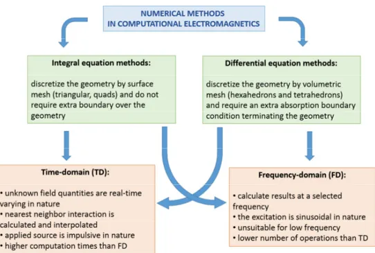
2. Numerical methods in computational electromagnetic ... 33

3. Numerical investigation of zone plates for terahertz focusing ... 35

3.1 Material choice ... 37

3.2 Number of zones ... 37

3.3 Frequency behavior ... 38

3.4 Comparison with a conventional refractive lens ... 39

4. Fabrication ... 39

CHAPTER IV Numerical investigation and fabrication of terahertz zone plates ... 42

1. Material choice ... 42

2. Number of zones ... 43

(5)

V

4. Comparison with a conventional refractive lens ... 46

5. Conclusions about the numerical investigation and zone plates fabrication .... 47

CHAPTER V Methods for the experimental characterization of diffractive lenses at terahertz frequencies ... 49

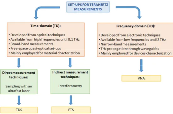
2. Set-ups for terahertz metrology ... 50

2.1 Set-ups employing time-domain methods ... 51

2.2 Set-ups employing frequency-domain methods ... 51

3. Terahertz diffractive lenses characterization: measurements set-up ... 53

4. Terahertz beam characterization: knife-edge technique... 56

4.1 Knife-edge set-up ... 56

4.2 Knife-edge measurements automation ... 59

4.3 Post-processing of data from knife-edge measurements: terahertz imaging 61 5. Iris sampling method: focal length characterization ... 62

6. Terahertz spectrometer calibration ... 63

6.1 Near-field antenna images on cross-sections of emitted radiation ... 64

6.2 Distribution of the field intensity employed as lenses excitation ... 64

CHAPTER VI Experimental characterization of polymeric zone plates ... 67

2. Zone plates focal length ... 67

3. Zone plates focal plane ... 69

4. Focal plane experimental comparison between ideal and real illumination: multilevel zone plate case of study ... 72

5. Conclusions ... 73

CHAPTER VII Future perspectives in developing planar diffractive lenses ... 74

(6)

VI

2. Tunable zone plates ... 74

2.1 Material with tunable properties: liquid crystals ... 75

2.1.1 Effects of an external electric field on nematic liquid crystals ... 77

2.1.2 Q-tensor formulation ... 79

2.2 Double-sided zone plate with two focal lengths ... 81

3. Metal zone plates ... 88

3.1 Zone plates in reflection mode ... 89

CHAPTER VIII Leaky-wave antennas for terahertz far-field applications ... 92

2. Historical path in the development of a leaky-wave theory ... 93

3. Classification of leaky-wave antennas... 95

3.1 One-dimensional uniform leaky-wave antennas ... 95

3.2 One-dimensional periodic leaky-wave antennas ... 97

3.3 Two-dimensional leaky-wave antennas ... 98

4. Operation principles of leaky waves ... 99

5. Leaky-wave antenna analysis and design techniques overview ... 102

5.1 Transverse resonance technique ... 104

6. Leaky-wave antennas at terahertz frequencies ... 105

CHAPTER IX Fabry-Perot cavity leaky-wave antennas based on liquid crystals for terahertz beam-steering ... 110

2. Liquid crystals for the design of a tunable leaky-wave antenna ... 111

3. Tunable Fabry-Perot cavity leaky-wave antenna design ... 114

4. Terahertz implementation of a Fabry-Perot cavity leaky-wave antenna with liquid crystals: numerical results ... 116 4.1 Dispersion analysis of fundamental leaky modes: lossless case of study117

(7)

VII

4.2 Terahertz Fabry-Perot cavity leaky-wave antenna radiation patterns:

lossless case of study ... 120

4.3 Terahertz Fabry-Perot cavity leaky-wave antenna: dispersion curves and radiation patterns in the case of materials with dielectric losses ... 122

CHAPTER X Terahertz leaky-wave antennas based on homogenized metasurfaces ... 126

2. Design constraints of terahertz metasurface leaky-wave antennas ... 127

3. Impedance synthesis of three partially reflective sheet geometries ... 130

4. Radiating behavior of Fabry-Perot cavity leaky-wave antennas based on fishnet-like metasurface ... 134

4.1 Full-wave analysis of the truncated structure ... 138

REFERENCES ... 142

LIST OF PUBLICATIONS ... 167

Journal papers ... 167

Conference proceedings ... 167

(8)

VIII

LIST OF FIGURES

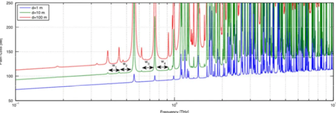
Fig. 1 Electromagnetic spectrum. ... 2 Fig. 2 Path loss in line-on-site communications at THz frequencies for different

distances. It takes into account both attenuation due to molecular absorption of gases in atmosphere both the spreading losses. Three bands are marked as promising ranges: 0.38 – 0.44 THz, 0.45 – 0.52 THz, 0.62 – 0.72 THz, and 0.77 – 0.92 THz [29]. ... 4

Fig. 3 Comparison between novel polarizers (red) and commercially available

polarizers (blue) at the frequency of 1 THz. Figure is taken from [91] where a description of the polarizers in the legend is driven in detail. ... 14

Fig. 4 Behavior of some filter categories widely employed at THz frequencies [88]. . 16 Fig. 5 Huygens-Fresnel principle for zone plate construction. A plane wave is

propagating towards the point of the space P0. O, R1, and R2 are point of the wave front, which have a fixed distance with respect to P0... 18

Fig. 6 a) Fresnel ZP for a microlight emitting diode [119]; b) ZP constructed for 12-cm

waves [120]. ... 20

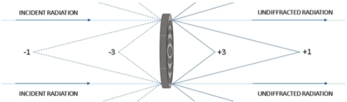
Fig. 7 Multiple and virtual foci in a ZP. Undiffracted radiation is commonly called

zero-order of diffracted radiation. The focus “+1” is associated to the first order of diffraction. The focus “+3” represents a higher-order focus, corresponding to i = 2 in equation II.8. Foci “-1” and “-3” are the equivalent virtual foci of the positive ones. .. 25

Fig. 8 Diffraction efficiency by increasing the number of discretization of zones phase

step [117]. ... 32

(9)

IX

Fig. 10 Comparison between sources in terms of frequency and output power. This

plot is from [5] and it is based on data until the year 2011. For additional information about THz sources until the year 2017, compare Table 1. ... 38

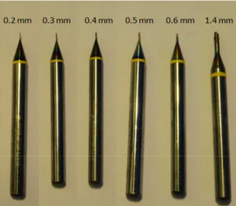
Fig. 11 Milling cutters used throughout this work for ZP fabrication. The diameter of

each cutter is indicated. ... 41

Fig. 12 Comparison between the focusing properties of a binary ZP made of a) Zeonex

E48R and b) HRFZ-Si. A plane wave of 1 V/m is incident perpendicularly to both lenses. The E-field modulus is represented in a 3-D space, filled by air. Both ZPs, ending at z = 2 mm, have same external diameter, number of zones and thickness. ... 42

Fig. 13 Comparison between the focusing properties of a binary ZP made of Zeonex

E48R (blue line) or HRFZ-Si (red line). A plane wave of 1 V/m is incident perpendicularly to both lenses. z-axis is the perpendicular one to the ZP plane. z = 0 mm corresponds to the end of the lens, where a free space, filled by air, starts. Both ZPs have the same external diameter, number of zones and thickness. ... 43

Fig. 14 Focusing behavior of a binary ZP with a fixed diameter and an increasing

number of ring zones. A plane wave of 1 V/m is incident perpendicularly to the lens. All color maps represents ZP central section and optical axis, z, where THz radiation, coming from z = 0, is focused. ... 45

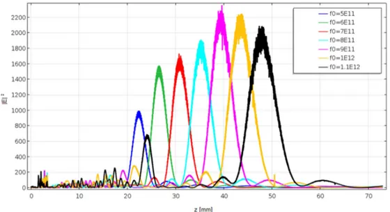
Fig. 15 Frequency behavior of a multilevel ZP from 0.5 THz to 1.1 THz with a step of

0.1 THz. z-axis is the perpendicular one to the ZP plane. Minor peaks in the square modulus of the E-field for z from 1 mm to 3 mm are related to multiple reflections within the 2 mm thick slab in which ZP is fabricated (no antireflection coating is used). For z < 1 mm and z > 3 mm, a free space filled by air for THz waves propagation is considered. ... 46

Fig. 16 Frequency behavior of a biconvex refractive lens from 0.5 THz to 1.1 THz

with a step of 0.1 THz. z -axis is the lens optical axis. Extremely short peaks in the square modulus of the E-field for z from 2 mm to 4 mm are related to few multiple reflections inside the lens. For z < 2 mm and z > 4 mm, a free space, filled by air, for THz waves propagation is considered. ... 47

(10)

X

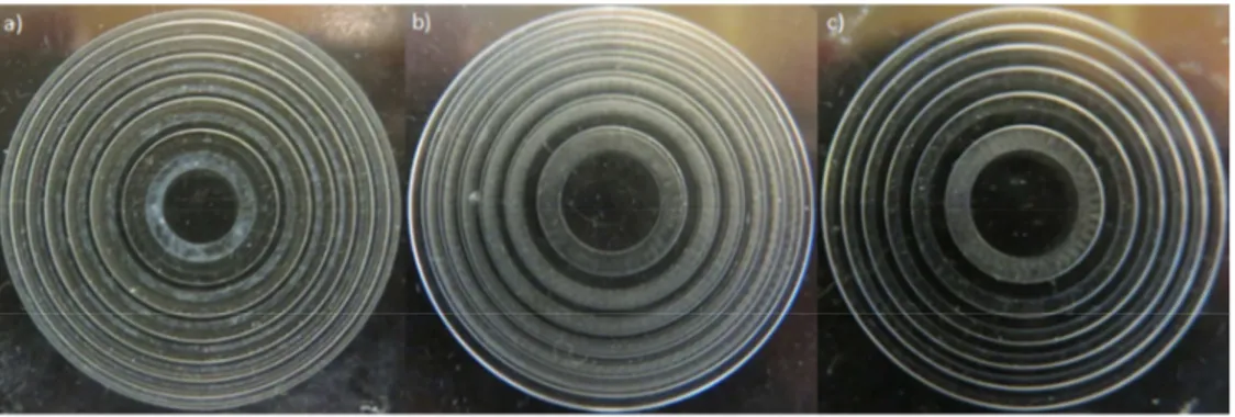
Fig. 17 Fabricated ZP lenses: a) multilevel ZP, b) double-sided ZP, c) binary ZP. The

little roughness perceived in visible light is introduced by milling process, but it does not affect the lens behavior at THz because it is several orders of magnitude below the wavelength at 1 THz. ... 48

Fig. 18 Overview of the experimental approaches to the THz measurements. ... 50 Fig. 19 Schematic representation of photoconductive antennas in their a) emitting and

b) receiving configuration. PI is the photogenerated current. ... 54

Fig. 20 Standard configuration of the commercial TDS TERA K15 by Menlo Systems.

PAT: photoconductive antenna in transmission mode; L1 and L3: convex-plane lenses; L2 and L4: plano-convex lenses; PAR: photoconductive antenna in receiving mode [180]. ... 55

Fig. 21 TDS set-up configurations for the characterization of the THz beam emitted by

the lens antenna (PAT). Three planes are imaged by knife-edge technique: a) plane 1, at a distance of 3 mm from the PAT; b) plane 2, at a distance of 9 mm from the PAT; c) plane 3, at the position in which the test ZPs will be located. PAT: photoconductive antenna in transmission mode; L1 and L3: convex-plane lenses; L2 and L4: plano-convex lenses; KE: knife-edge blade; PAR: photoconductive antenna in receiving mode... 57

Fig. 22 Schematic representation of a THz TDS for focal spot measurements. PAT:

photoconductive antenna in transmission mode; L1 and L3: convex-plane lenses; L4: plano-convex lens; KE: knife-edge blade; PAR: photoconductive antenna in receiving mode... 58

Fig. 23 Experimental set-up for standard knife-edge measurements. PAT:

photoconductive antenna in transmission mode; L1 and L3: convex-plane lenses; L4: plano-convex lens; KE: knife-edge blade; PAR: photoconductive antenna in receiving mode... 59

Fig. 24 LabVIEW front panel for knife-edge measurements automation. It employs

(11)

XI

several parameters. Program also shows an updated plot of saved data and blade position. ... 60

Fig. 25 Schematic representation of a THz TDS for focal length measurements. PAT:

photoconductive antenna in transmission mode; L1 and L3: convex-plane lenses; L4: plano-convex lens; I: iris; PAR: photoconductive antenna in receiving mode. ... 62

Fig. 26 Field distribution at 1 THz at a) 3 mm and b) 9 mm from the hemispherical

lens of the emitting photoconductive antenna... 64

Fig. 27 THz field distribution collimated by a commercial lens and imaged on a planar

surface by knife-edge technique. ... 65

Fig. 28 Experimental and numerical evaluation of the focal length of three ZPs by

means of the optical axis sampling of a) binary ZP, b) double-sided ZP, and c) multilevel ZP. Measurements are performed with the iris sampling method, which is also reproduced in the simulation environment. ... 69

Fig. 29 Acquired data for a) a conventional binary ZP, b) a double-sided ZP, and c) a

multilevel ZP; their difference quotient for d) a conventional binary ZP, e) a double-sided ZP, and f) a multilevel ZP; and focal plane images obtained by knife-edge measurements for g) a conventional binary ZP, h) a double-sided ZP, and i) a multilevel ZP. Negative values of the |E|/|E|max are due to diffraction and scattering among the components in the THz optical path. ... 71

Fig. 30 Normalized amplitude of the electric field in the focal plane for the multilevel

ZP acquired with knife-edge technique by rotating a) the lens, or b) the blade. ... 73

Fig. 31 Liquid crystals mesophases: a) nematic, b) cholesteric, and c) smectic. ... 76 Fig. 32 Orientation of rod-like molecules in a nematic LC cell without any applied

voltage or in presence of a voltage with strength higher than Freedericksz threshold. Typically, an alternating voltage in the few kilohertz range is chosen for preventing electrochemical degradation. ... 78

(12)

XII

Fig. 33 a) A ZP configuration with a uniform electrode on top and a ZP-patterned

electrode on bottom substrate. The rest condition of the LC is tilted 2° from the y-axis. b) tilt angle and c) y-component of refractive index tensor distributions in a LC cell 387 µm thick, 2 ms after the application of a 70 V step voltage (steady state). ... 83

Fig. 34 a) A ZP configuration with a uniform electrode on top and a ZP-patterned

electrode on bottom substrate. The rest condition of the LC is tilted 2° from the y-axis. b) tilt angle and c) y-component of refractive index tensor distributions in a LC cell 193 µm thick, 2 ms after the application of a 35 V step voltage (steady state). ... 84

Fig. 35 Cross section of geometrical radial-symmetric model and data for the materials

chosen for a dual-focus double-sided ZP. The ZP is symmetric and only the profile along the radius of the lens is represented in the picture. ... 86

Fig. 36 Computed square modulus of the electric field component along the optical

axis (z-component) at 1 THz for a dual-focus double-sided phase-reversal ZP lens. The green line is for zero applied voltage (rest), while the blue line is for LC molecules parallel to the lens optical axis (V∞). ... 86

Fig. 37 Computed normalized square modulus of the z-component of the electric field

at 0.5 THz along the optical axis of a Fresnel ZP working in transmission (red) or in reflection mode (blue). ... 90

Fig. 38 Comparison between the computed square module of the electric field

normalized to the square module of the incident electric field, at 0.5 THz, along the optical axis of a Fresnel ZP reflector and a multilevel phase-reversal ZP (compare Ch. IV). ... 90

Fig. 39 A rectangular waveguide, as an example of 1-D uniform LWAs. The

electromagnetic field propagates in z-direction. An infinite ground plane surrounds the slot [222]. ... 96

Fig. 40 An example of periodic 1-D LWA. This antenna configuration has a width, w,

larger than the operative wavelength. The electric field is in y-direction and the electromagnetic wave propagates in z-direction. ... 97

(13)

XIII

Fig. 41 An example of a 2-D LWA: the substrate-superstrate LWA. It can produce a) a

pencil beam at broadside or b) a conical beam with an angle θ with respect to the broadside direction. ... 98

Fig. 42 Ray diagram of a forward leaky-wave. The intensity of the field is given by

arrows separation: closer arrows correspond to a stronger field [222]. ... 100

Fig. 43 Ray diagram of a backward leaky-wave. The intensity of the field is given by

arrows separation: closer arrows correspond to a stronger field [222]. ... 101

Fig. 44 Ray diagram of a leaky-wave excited by a source located in z = 0 [222]. ... 101 Fig. 45 Terminated equivalent network representing a waveguide cross-section [223].

... 104

Fig. 46 LC cell driven by a gold fishnet electrode. ... 111 Fig. 47 Real part of the three main components of the LC permittivity tensor mapped

in the xy-plane, in the middle of the LC cell (z = 0). The LCs behavior is show in absence of an external field (first row), for a voltage above the threshold (last row), and for an intermediate value of driving voltage (middle row) [with courtesy of Dr. W. Fuscaldo]. ... 112

Fig. 48 Real and the imaginary part of the LC dielectric permittivity along a line

perpendicular to the xy-plane and passing through three selected points of the LC cell [with courtesy of Dr. W. Fuscaldo]. ... 113

Fig. 49 Schematic representation of the proposed FPC-LWA and its equivalent

transmission line model. ... 115

Fig. 50 Dispersion curves of the fundamental TM for different THz FPC-LWA with

LC: a) Layout 1, b) Layout 2, c) Layout 3, d) Layout 4. Colors gradually shade from blue to red as the applied external voltage decreases from V∞ to zero [with courtesy of Dr. W. Fuscaldo]. ... 118

(14)

XIV

Fig. 51 Radiation patterns predicted by leaky-wave theory (dashed lines) or by means

of reciprocity theorem (solid lines): a) Layout 1, b) Layout 2, c) Layout 3, and d) Layout 4 (see Table 3.5). The condition of the THz beam pointing at broadside (blue lines) and the radiation at the maximum pointing angle (red lines) are presented [with courtesy of Dr. W. Fuscaldo]. ... 121

Fig. 52 Dispersion curves of the fundamental TM when losses of the materials are

taken into account: a) Layout 2, and b) Layout 4. Colors gradually shade from blue to red as the applied external voltage decreases from V∞ to zero [with courtesy of Dr. W. Fuscaldo]. ... 122

Fig. 53 THz FPC-LWA unit cell model, as implemented in CST full-wave simulation.

A probe for evaluating the tangential magnetic field at the ground plane is added as a light blue arrow. ... 123

Fig. 54 Radiation patterns of a) Layout 2 and b) Layout 4 for radiation at broadside

(solid) and at the maximum pointing angle (dashed). Radiation patterns are calculated by means of reciprocity theorem in the lossless (in red) and the lossy (in black) case. Patterns from leaky-wave theory are also shown (blue). Full-wave simulations with CST are reported, in the lossy case, for radiation at broadside (filled green circles) and at the maximum pointing angle (empty green circles) [with courtesy of Dr. W. Fuscaldo]. ... 124

Fig. 55 Directivity at broadside as a function of the characteristic impedance of a PRS

(see equation X.1). Black, blue, green, and red dashed lines selects the reactance values required for achieving theoretical directivities of 15, 20, 25 and 30 dB, respectively. ... 128

Fig. 56 A model for evaluating the surface impedance of a periodic PRS. A Floquet

wave impinges on the PRS. The impedance matrix is obtained in correspondence of the PRS, fixing a suitable de-embedding distance. An equivalent circuit model can be derived for retrieving the value of the surface impedance from the impedance matrix parameters. ... 129

(15)

XV

Fig. 57 Illustrative example of a FPC-LWA based on PRS with three different

elements geometry. ... 130

Fig. 58 Surface reactance Xs of a) a patch-based PRS, as a function of the normalized

gap g between the patches, and b) a strip-based PRS, as a function of the normalized width w of the strips. ... 131

Fig. 59 Surface reactance Xs of a fishnet-based PRS as a function of both g and w. The

iso-lines of the reactance at 15, 25, 45, and 75 Ω are reported in white dashed lines. 132

Fig. 60 Surface reactance of a fishnet-like unit cell as a function of frequency. The

family of curves is obtained changing the angle of incidence from 0° to 80° (the color shades from blue to red, respectively). ... 133

Fig. 61 a) Surface reactance as a function of the frequency for the four layouts

presented in Table 14: behavior at 15 Ω is in red, at 25 Ω is in blue, at 45 Ω is in green, and at 66 Ω is in black. b) Section of the proposed FPC-LWA and its equivalent circuit model. Z0 and Z1 are the modal impedances in the air and in the medium, respectively, whereas kx0 and kx1 are the vertical wavenumbers in the air and in the medium,

respectively. ... 135

Fig. 62 Dispersion curves βz/k0 (solid lines) and αz/k0 (dashed lines) as a function of the frequency. In the insets, the frequency range is limited to 0.8 – 1.2 THz to highlight the behavior around the operative frequency of the dominant leaky modes for both TE (in green) and TM (in blue) polarizations. ... 135

Fig. 63 Radiation patterns normalized to broadside radiation calculated with the

leaky-wave approach (black solid lines) and reciprocity theorem (black dashed lines) are reported over the E-plane for the four layouts of Table 14. ... 136

leaky-wave approach (black solid lines) and reciprocity theorem (black dashed lines) are reported over the H-plane for the four layouts of Table 14. ... 137

(16)

XVI

with full-wave simulations (black circles) are reported over the E-plane for the four layout of Table 14. ... 139

leaky-wave approach (red solid lines) and reciprocity theorem (blue asterisks), and validated with full-wave simulations (black circles) are reported over the H-plane for the four layout of Table 14. ... 140

(17)

XVII

LIST OF TABLES

Table 1 Comparison between the main THz radiation sources. ... 7 Table 2 Comparison between some techniques employing optical and near-infrared

lasers for generating THz radiation by optical pumping. ... 8

Table 3 Commercially available THz time-domain spectrometers generating THz

radiation by photoconductive antennas (readapted from [76]). ... 9

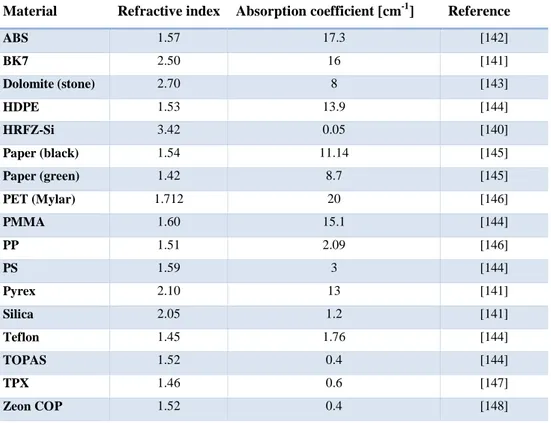
Table 4 Commercial available detectors for THz radiation [25]. ... 10 Table 5 Comparison of THz conventional materials refractive index and absorption

coefficient at 1 THz. ... 27

Table 6 Dependence of the number of operations to the frequency f and the number of

iterations Nit [161]. ... 33

Table 7 Comparison between lenses fabrication techniques [167]. ... 40 Table 8 Leaky-wave antennas typologies and examples, working in the frequency

range of 0.3 - 3 THz. In the headers, f is the frequency at which the antennas are investigated, while η is the radiation efficiency. ... 106

Table 9 Metasurfaces FPC-LWAs in the frequency range 0.3 - 3 THz. In the headers, f

is the frequency at which the antennas are investigated, while η is the radiation efficiency. ... 107

Table 10 Leaky-wave antennas with a reconfigurable pointing angle, working in the

frequency range between about 0.3 THz and 3 THz. In the headers, f is the frequency at which the antennas are investigated, η is the radiation efficiency, and ∆θ is the maximum variation of the pointing angle. ... 108

(18)

XVIII

Table 12 Figure of merits for radiating performance of different layouts of a

FPC-LWA with LCs: beam reconfigurability (θpM), directivity (D0) and beamwidth (∆θ). 119

Table 13 Comparison between radiation properties of Layout 2 and 4, with and

without dielectric material losses. ... 124

Table 14 Relevant geometrical parameters and radiating properties of the FPC-LWAs

(19)

XIX

ABSTRACT

The terahertz frequency electromagnetic radiation has gathered a growing interest from the scientific and technological communities in the last 30 years, due to its capability to penetrate common materials, such as paper, fabrics, or some plastics and offer information on a length scale between 100 µm and 1 mm. Moreover, terahertz radiation can be employed for wireless communications, because it is able to sustain terabit-per-second wireless links, opening to the possibility of a new generation of data networks.

However, the terahertz band is a challenging range of the electromagnetic spectrum in terms of technological development and it falls amidst the microwave and optical techniques. Even though this so-called “terahertz gap” is progressively narrowing, the demand of efficient terahertz sources and detectors, as well as passive components for the management of terahertz radiation, is still high. In fact, novel strategies are currently under investigation, aiming at improving the performance of terahertz devices and, at the same time, at reducing their structure complexity and fabrication costs.

In this PhD work, two classes of devices are studied, one for near-field focusing and one for far-field radiation with high directivity. Some solutions for their practical implementation are presented.

The first class encompasses several configurations of diffractive lenses for focusing terahertz radiation. A configuration for a terahertz diffractive lens is proposed, numerically optimized, and experimentally evaluated. It shows a better resolution than a standard configuration. Moreover, this lens is investigated with regard to the possibility to develop terahertz diffractive lenses with a tunable focal length by means of an electro-optical control. Preliminary numerical data present a dual-focus capability at terahertz frequencies.

The second class encompasses advanced radiating systems for controlling the far-field radiating features at terahertz frequencies. These are designed by means of the formalism of leaky-wave theory. Specifically, the use of an electro-optical material is considered for the design of a leaky-wave antenna operating in the terahertz range,

(20)

XX

achieving very promising results in terms of reconfigurability, efficiency, and radiating capabilities. Furthermore, different metasurface topologies are studied. Their analytical and numerical investigation reveals a high directivity in radiating performance. Directions for the fabrication and experimental test at terahertz frequencies of the proposed radiating structures are addressed.

(21)

XXI

ACKNOWLEDGMENTS

The work described in this PhD thesis has been possible thanks to the help and the support of several people.

At first, I would like to thank my supervisors, prof. Alessandro Galli and Dr. Romeo Beccherelli, for their suggestions and patience during these three years.

I thank prof. Renato Cicchetti, prof. Emanuele Piuzzi, and prof. Antonio d’Alessandro from Department of Information Engineering, Electronics and Telecommunications of “Sapienza” University, who have been members of my Advisory Board, for their valuable doubts and questions.

I thank Alfonso Morbidini from Istituto Nazionale di Astrofisica (INAF) for his willingness and the time he spent for the lenses fabrication.

I thank Dr. Mauro Missori from Istituto dei Sistemi Complessi of Consiglio Nazionale delle Ricerche (ISC-CNR) and prof. Renato Fastampa from Physics Department of “Sapienza” University for their precious supervision and help during terahertz experimental measurements.

I thank Dr. Dimitrios Zografopoulos from Istituto per la Microelettronica e Microsistemi of Consiglio Nazionale delle Ricerche (ISC-CNR) for the time he spent teaching me the numerical tools employed in the study of liquid crystals.

I thank Dr. Walter Fuscaldo from Department of Information Engineering, Electronics and Telecommunications of “Sapienza” University for introducing me, with patience and dedication, in the field of leaky-wave antennas.

I thank my labmates for the stimulating discussions and for all the fun we have had together.

Last but not the least, I would like to thank my family, my boyfriend and my friends for supporting me spiritually throughout this PhD and my life in general.

(22)

XXII

LIST OF SYMBOLS,

ABBREVIATIONS AND

ACRONYMS

Symbols

angle between the optical axis and the principal ray attenuation constant due to material losses

radial attenuation constant

attenuation constant in z-direction

normalized attenuation constant phase constant vector

radial phase constant

phase constant in x-direction phase constant in z-direction normalized phase constant

ratio between the viscosity of a nematic liquid crystal and the order parameter

scattering frequency

Δ dielectric anisotropy

∆θ beamwidth

∆λ interval of wavelengths

Δ transverse wavenumber perturbation

∆n birefringence

∆r width of the outermost ring of a zone plate

̿ dielectric permittivity tensor

dielectric permittivity in direction perpendicular to the polarization direction of an applied electric field ∥ dielectric permittivity in direction parallel to the

(23)

XXIII

polarization direction of an applied electric field vacuum dielectric permittivity

extraordinary dielectric permittivity average dielectric anisotropy ordinary dielectric permittivity

̃ relative dielectric permittivity

radiation efficiency

diffraction efficiency

vacuum impedance

θ azimuthal angle

angle between the z-axis and the phase vector

θm angle between the long molecular axes of a liquid crystal and its director

beam reconfigurability

λ wavelength

wavelength in vacuum

!,#,$ eigenvalues of the Q-tensor

% wavelength in an alumina layer

& arbitrary wavelength value in a wavelength range

'( wavelength in a liquid crystal layer

)* wavelength in a polymeric substrate

+ vacuum permeability σ electric conductivity , phase shift - angular frequency -. plasma frequency A arbitrary constant

a radius of the central circle of a zone plate

ath thermotropic coefficient

bth thermotropic coefficient

cth thermotropic coefficient

(24)

XXIV

D electromagnetic displacement vector

D dissipation function

D0 directivity

E electric field

EF electric field for the Freedericksz transition

Em average electric field

Emax maximum electric field

/ efficiency

/ ,0 efficiency contribution due to the substrate losses

ER extinction ratio

f frequency

f/# f-number of a lens

f0 design frequency

12 free energy density

1 elastic energy density

13 electromagnetic energy density

fop operating frequency

14 thermotropic energy density

G gain

g gap

ℎ6 convolution kernel

hair distance between the unit cell and the waveguide port

hi thickness of the i-th layer

i positive integer

7̿ identity matrix

K local field factor

free-space wavenumber radial wavenumber propagation wavenumber

8 transverse wavenumber

8 transverse wavenumber of an unperturbed mode

(25)

XXV

L straight line

L1 collimating refractive lens

L1,2,6 elastic parameters

L2 focalizing refractive lens

L3 collimating refractive lens

L4 focalizing refractive lens

m number of Fresnel zones

m integer (only in chapters VIII, IX, and X)

m director of the short molecular axis

N number of layers in a multistack

n refractive index

n integer (only in chapter IX)

n director of the long molecular axis

ne extraordinary refractive index

no ordinary refractive index

Nit number of iterations

p object distance

p period (only in chapters VIII and X)

p integer (only in chapters IX)

p1,2 polarization coefficients P polarization vector Pd diffracted power PI photogenerated current Pin incident power q image distance 9: Q-tensor qi i th

element of the Q-tensor

;< responsivity

S order parameter

Seq order parameter in the equilibrium state

t thickness

(26)

XXVI

TTM transverse-magnetic component of transmitted power

V∞ asymptotic value of the voltage for an infinite time

VF voltage for the Freedericksz transition

Vi voltage signal of the i

th

pixel of a detector array

=> voltage spectral dentisity

w width

Xs surface reactance

Y admittance

Y’ normalized admittance

Y0 admittance in vacuum

Z impedance

Z’ normalized impedance

Z0 impedance in vacuum

Zi,j elements of the impedance matrix of a two-port

network

Zin input impedance

ZL characteristic impedance of the Floquet port in the substrate Zs surface impedance Units of measurements µm micrometers µW microwatt cm centimeter dB decibel

fps foot per second

fs femtosecond

GB gigabyte

GHz gigahertz

Hz hertz

(27)

XXVII kΩ kiloohm kHz kilohertz km kilometer kW kilowatt m meters mm millimeter mPa millipascal ms millisecond MW megawatt mW milliwatt nm nanometer ns nanosecond nW nanowatt pN piconewton ps picosecond pW picowatt rad radian s second S siemens THz terahertz V volt W watt

Chemical symbols and formulas

Au gold

Al aluminum

Al2O3 alumina

CF4 tetrafluoromethane

Cr chromium

GaAs gallium arsenide

(28)

XXVIII

InGaAs indium gallium arsenide

LiTaO3 lithium tantalite

Ni nickel

p-Ge germanium doped with an acceptor

SF6 sulfur hexafluoride

Si silicon

SiNx silicon nitride

SiO2 silica

Ti titanium

VOx vanadium oxide

Abbreviations

c.w. continuous wave

e.g. exempli gratia

Fig. figure i.e. id est min minutes viz. videlicet Acronyms 1D, 1-D one-dimensional 2D, 2-D two-dimensional 3D, 3-D tridimensional

ABS acrylonitrile butadiene styrene

AF array factor

CAD computer-aided drafting

CMOS complementary metal-oxide semiconductor

CNT carbon nanotubes

(29)

XXIX

DBR distributed Bragg reflector

DC direct current

DNA deoxyribonucleic acid

EBG electronic bandgap

FBW fractional bandwidth

FD frequency domain

FDTD finite difference time domain

FEM finite element method

FET field-effect transistor

FF filling factor

FIT finite integration technique

FPA focal-plane array

FPC Fabry-Perot cavity

FTIR Fourier transform infrared spectrometer

FTS fast tool servo (only in chapter III)

FTS Fourier transform spectroscopy

FWHM full width at the half maximum

Gbps gigabit-per-second

GDS grounded dielectric slab

HD high definition

HDPE high-density polyethylene

HEMT high electron mobility transistor

HMD horizontal magnetic dipole

HPBW half power beamwidth

HRFZ high resistivity floating zone

HSS high-speed steel

IR infrared

ITO indium tin oxide

KE knife-edge

LC liquid crystals

LEO low Earth orbit

LOS line-on-site

(30)

XXX

MM micro-milling

MMW millimeter-waves

MoM method of moments

MOSFET metal-oxide-semiconductor field-effect transistor

MPIE mixed-potential integral equation

NEP noise equivalent power

QCL quantum cascade laser

QW quantum well

PAR photoconductive antenna in reception mode

PAT photoconductive antenna in transmission mode

PEDOT:PSS poly(3,4-ethylenedioxythiophene):poly(4- styrenesulfonate)

PEC perfect electric conductor

PET polyethylene terephthalate

PGF periodic Green’s function

PMMA poly(methyl methacrylate)

PP polypropylene

PRS partially reflective sheet

PS polystyrene

PTFE polytetrafluoroethylene

RAM random access memory

RIE reactive ion etching

RT Radon transform

SNR signal-to-noise ratio

SPDT single point diamond turning

STS slow tool servo

Tbps terabit-per-second

TD time domain

TDS time domain spectrometer, time domain spectroscopy

TE transverse-electric

TEN transverse equivalent network

TM transverse-magnetic

(31)

XXXI

TRT transverse resonance technique

US$ USA dollars

UV ultraviolet

VGA video graphics array

VIS visible

VNA vector network analyzer

WG waveguide

WP waveplate

(32)

XXXII

INTRODUCTION

“Since we have become accustomed to think of waves of electrical energy and

light waves as forming component parts of a common spectrum, the attempt has often been made to extend our knowledge over the wide region which has separated the two phenomena, and to bring them closer together, either by cutting down the wave length of electrical oscillations […] or by the discovery and measurement of longer heat waves.”

― H. Rubens and E.F. Nichols1, 1897.

This statement is the opening of a significant paper for the development of a terahertz science. Even though this was only a first stage, it was clear that there were two approaches for the development of a terahertz technology: the optical and the electronic route. The terahertz range has been associated for long time to its lack in technical capabilities. It was only during 1970s that the first terahertz benchtop set-ups suitable for spectroscopic investigations have been developed. This was the starting point for the experimental test of passive components and detectors, which have been allowed for reducing the technological gap.

Nowadays, terahertz radiation has become crucial in several fields, such as, for example, the objects inspection for industrial and security applications or the wireless communications. Thus, there is a high requirement of affordable high-performance terahertz devices, suitable for mass production and for the integration in complex systems.

The Chapter I introduces the terahertz radiation, starting from a definition of the frequency band and its main application fields, passing through the state-of-art of terahertz generation and detection, and concluding with a brief overview of the most employed passive components for terahertz radiation. Among them, this PhD thesis is devoted to the development of planar diffractive lenses. Thus, the Chapter II discusses

1_{H. Rubens and E.F. Nichols, “Heat rays of great wave length,” Phys. Rev. (Series I), vol. 4,}

(33)

XXXIII

this choice, comparing the diffractive lenses with the most conventional refractive lenses and parabolic mirrors for terahertz focusing. Moreover, the Chapter II provides the theoretical background of diffractive lenses design, as well as an overview of the materials and the fabrication processes suitable for their practical implementation. The numerical investigation of the diffractive lenses is described in Chapter III. It aims at optimizing the lenses geometry and comparing their behavior with the one of a refractive lens of equal diameter. The numerical data coming from this analysis are reported and discussed in Chapter IV and constitute the design basis for their fabrication. The available experimental techniques for terahertz characterization are introduced in Chapter V, which also includes the description and the calibration of the available instrument and of the set-up built for the lenses measurements. The data resulting from the experimental characterization of the fabricated lens prototypes are reported in Chapter VI.

The design and the experimental characterization presented in Chapters III-VI are the starting point for a preliminary study on advanced diffractive lens configurations, such as a tunable dual-focus diffractive lens and a diffractive lens working in reflection mode (Chapter VII). This last device opens also the possibility to design terahertz lens antennas employing such diffractive lenses.

In terms of radiating systems for terahertz applications, an interesting device is the Fabry-Perot cavity leaky-wave antenna. It has the advantage to be scalable from microwaves to optical frequencies, due to the ubiquity of the leaky-wave phenomena (introduced in Chapter VIII). Thus, two main configurations of Fabry-Perot cavity leaky-wave antenna are presented for working at terahertz frequencies. In Chapter IX, a leaky-wave antenna based on a multistack of isotropic and anisotropic material layers is theoretically investigated for steering the THz beam. In Chapter X, leaky-wave antennas made with different metasurface topologies are theoretically studied for the design of high directivity terahertz antennas. Furthermore, their practical implementation is discussed.

(34)

(35)

1

CHAPTER I

Terahertz radiation

1. Introduction to terahertz radiation

The so-called terahertz (THz) radiation is an electromagnetic radiation with a frequency between 100 GHz and 10 THz [1]–[5]. However, this definition is not completely accepted and the THz range is sometimes extended from 100 GHz to 30 THz [6] or limited to a narrower region, between 300 GHz and 3 THz. About this issue, in 2002 Siegel wrote [7]: “Below 300 GHz, we cross into the millimeter-wave bands (best delimited in the author’s opinion by the upper operating frequency of WR-3 waveguide — WR-3WR-30 THz). Beyond WR-3 THz, and out to WR-30 µm (10 THz) is more or less unclaimed territory, as few if any components exist. The border between far-IR and submillimeter is still rather blurry and the designation is likely to follow the methodology (bulk or modal — photon or wave), which is dominant in the particular instrument.”

Sometimes, the designation of a range as THz frequencies band is influenced by the specific field of application. For example, the technological interest towards THz radiation arose in connection with the development of space-based instruments for astrophysics and Earth missions. The 98% of total photons emitted in the history of the Universe since the Big Bang has a frequency below 30 THz, with a peak emission at around 3 THz (cosmic microwave background radiation, which have a spectral radiance peak at about 160 GHz [8], is excluded) [3], [5]. For this reason, in this field, 30 THz can be considered the upper limit of the THz band. However, most of the scientific and technological community refers as THz the radiation between 300 GHz and 10 THz.

(36)

2

1.1Terahertz in the electromagnetic spectrum

A first experimental effort towards material characterization by THz radiation was in 1897 [9], [10]. It consisted of measurements of black body radiation employing a bolometer. In [10], the authors wrote: “since we have become accustomed to think of waves of electrical energy and light waves as forming component parts of a common spectrum, the attempt has often been made to extend our knowledge over the wide region that separates the two phenomena, and bring them closer together”. It appears as a first explicit reference to the fact that a technological gap exists in the electromagnetic spectrum. It is set between photonics and electronics (Fig. 1).

Fig. 1 Electromagnetic spectrum.

A summary of the historical developments in this range of the spectrum is beyond the aim of the preset work. An interesting review can be found in [11]. However, it may be worthy to mention the key discoveries that contribute to the establishment of a THz technology. The first THz detectors were initially proposed for FIR radiation sensing. In 1959, the first carbon bolometer [12] as well as a photoconductive detector [13] were developed. During 1960s, several progresses were achieved in the field of detection: germanium bolometer [14], pyroelectric [15] and tunable FIR detectors [16] were introduced. With regard to the generation of THz radiation, in 1962, optical rectification mechanism was experimentally demonstrated for the first time [17]. It is still now one of the main THz generating mechanism [18]. In 1971, the first THz pulse was generated using a benchtop resource [19]. Finally, in 1984, the first laser operating

(37)

3

between 390 – 1000 µm was constructed, with a peak power up to 10 kW [20], whereas, in 1986, a THz emitting antenna was demonstrated for the first time [21]. Several progresses have been made until now in the field of THz sources and detectors. Starting from the 1950s, many attractive applications have been developed, as will be described in the following sections.

1.2Terahertz applications and challenges

Historically, THz detection was conceived for interstellar dust sensing between 100 GHz and 3 THz. Nowadays, space-borne THz sensors have been developed both for interstellar and Earth observation. Associated payload can be located at different orbits. Low Earth orbit (LEO, i.e., an orbit around Earth with an altitude of 2000 km or less, and an orbital period of about 84 – 127 min) allows for astronomy research [22] and Earth control [23]. Large space observatories [24] have more distant and relatively stable dislocation points and are usually devoted to deep space astronomy. In this situation, there are important limitations in terms of maximum mass (few tens of kilograms) and power supply availability (tens of watts) per instruments. Miniaturization, integration, and the employment of materials able to guarantee sensitivity and responsivity (see Ch. I Sec. 3) at high temperatures, are the main goal of THz technology for space application [25].

The THz measurements for Earth observations from LEO suffer from radiation attenuation due to water molecules absorption. Generally, water molecules in atmosphere create small clusters by means of hydrogen bonds. The rotation and vibration of water molecules in clusters determine absorptions in THz radiation spectrum. The number of molecules in the cluster establishes at which THz frequency there will be radiation absorption. For example, a cluster of 38 water molecules causes absorption at 20 THz [26], a cluster of 8 water molecules is responsible of absorption at 1.4 THz [27], while a mixture of ring clusters of 4, 5 and 6 molecules gives absorption lines at 0.56 THz, 0.76 THz, 0.98 THz, 1.1 THz, 1.17 THz, and 1.41 THz [28].

Due to water absorption, THz radiation can be exploited only in specific spectral bands for wireless communication. Most promising bands, for line-on-site (LOS) data

(38)

4

transmission at distances over 1 m, are in the ranges 0.38 – 0.44 THz, 0.45 – 0.52 THz, 0.62 – 0.72 THz, and 0.77 – 0.92 THz [29], as shown in Fig. 2. In these frequency windows, absorption losses due to atmosphere gases are below 10 dB/km, but spreading losses are high, motivating the requirement of high directivity and high gain antennas.

Fig. 2 Path loss in line-on-site communications at THz frequencies for different distances. It takes into

account both attenuation due to molecular absorption of gases in atmosphere both the spreading losses. Three bands are marked as promising ranges: 0.38 – 0.44 THz, 0.45 – 0.52 THz, 0.62 – 0.72 THz, and 0.77 – 0.92 THz [29].

The main advantage of wireless communication at THz is that wireless technology below 0.1 THz and above 10 THz is not able to sustain Terabit-per-second links (Tbps) [29]. In fact, below 0.1 THz, the available bandwidth is not sufficient and confines the feasible data rates. At millimeter waves (~ 60 GHz), 10 Gbps within 1 m are currently reachable [30], but they are of two orders of magnitude below the estimated demand in wireless communications of next future. On the other hand, above 10 THz, large bandwidth are available, but several limitations compromise the feasibility: (i) low transmission power due to eyes health safety; (ii) influence of atmospheric weather conditions on waves propagation; (iii) high reflection losses; (iv) losses due to emitter-receiver misalignment [31]. At THz frequencies, the main challenges for commercial realization of Tbps wireless technology are: (i) the realization of compact THz sources able to supply an output power in continuous wave mode up to 100 mW, and (ii) the availability of electronically steerable antenna arrays able to minimize link losses [25]. The THz technology is not completely mature yet, but these goals are reachable in the future.

(39)

5

From the point of view of biological applications, strong absorptions due to water molecules allow for the monitoring of water content in human tissues or the hydration level of plants [32]. Water allows for high contrast imaging at THz frequencies. With more detail, THz absorption depends on: (i) salts concentration; (ii) protein and DNA content; (iii) macromolecules structural changes, due to bonds with ligand or denaturing processes. Because all of these factors are also involved in the cellular metabolism, it is possible to distinguish between a healthy tissue and a tissue with a disease by means of THz radiation measurements [33]–[36]. Moreover, THz is a non-ionizing radiation and can be exploited for in vivo measurements. For example, one of the first applications in this field was presented in [37], where a change in skin hydration is detected in vivo by means of THz radiation. After that, THz radiation allowed for a high contrast imaging of hidden margins of basal cell carcinoma, a skin cancer, before a surgery intervention [38]. The THz radiation is able to penetrate under the skin in a non-invasive way and has a negligible scattering inside tissues. Moreover, time-domain systems (see next section) can offer quasi-3D information [25]. However, the availability of sources with yet limited power, when compared to the power required to cope with absorption due to water, confines THz penetration depth inside aqueous systems, such as human body. For this reason, at the present, THz radiation can be employed only for the diagnosis of superficial skin cancers.

The THz radiation has the great advantage to penetrate into non-metallic materials and to distinguish between them, thanks to specific band absorptions which provide a fingerprint for the material. In fact, THz radiation can be exploited for security applications and non-destructive packaging inspection. Examples of security applications are body-scanning imager [39] and explosives detection by spectrometer analysis [40]. Commercially available body-scanners work in the frequency range of 0.15 – 0.68 THz [41], [42] and have the advantages of being compatible with compact hardware systems, such as wearable devices. Moreover, they could combine imaging with spectroscopic information for the identification of dangerous substances. In fact, every molecule has its own fingerprint at THz frequencies, i.e. a unique spectrum of absorption due not only to the bounds between atoms in functional groups, but to the bound between atoms constituting a molecule [40]. However, in body-scanning, THz imaging detectors need to have an extremely large area, able to cover the dimensions of a human body. It constitutes a big issue, especially in the maintaining of good

(40)

6

imaging performance (compare Ch. I Sec. 3) with low times for image acquiring and affordable costs of the whole technology.

Penetrative capability of THz radiation in several common materials such as plastics, fabrics, ceramics, and paper, linked to the possibility to distinguish between them, can be applied in non-destructive and non-contact test of several objects and coatings. For example, marine structures are protected from environmental corrosion agents by specific coatings. The corrosive process is able to modify both chemical and physical properties of materials causing defects, as bubbles or cracks, which are usually located under the external surface of objects [43]. THz radiation is able to penetrate inside coatings and discloses every defect larger than the incident wavelength [44], [45]. In this way, it is possible to check coatings and prevent failures by substituting them before compromising the covered structure or object. By applying the same principles, it is also possible to employ THz radiation for monitoring and preserving the cultural heritage [46], [47]. Moreover, it is also possible to investigate under the surface of paintings or frescos and discover details hidden by their creator. THz spectroscopic imaging complements the information obtained by other consolidated techniques, such as the imaging at near-infrared frequencies. For example, in [48] a Pablo Picasso painting on canvas was analyzed by THz pulsed time-domain imaging. Different areas of this painting show different numbers of layer, confirming that the author repainted some parts of his artwork.

From a technological point of view, the main effort in the THz field is to provide a suitable source of radiation [49]. Available sources are usually expensive, bulky, and emit weak radiation. This problem can be approached from the millimeter-wave (MMW) side or from the infrared (IR) side [50]. From a MMW point of view, it is difficult at THz to create circuits for high-frequency waves. From an IR point of view, THz optical systems are challenging due to the fact that optical elements have dimensions comparable to the wavelength [51]. Some solutions and the state-of-art about THz sources will be discussed in the next section.

(41)

7

Table 1 Comparison between the main THz radiation sources. Frequency

[THz]

Output

power Advantages Disadvantages Reference

Direct generation Quantum cascade lasers 0.85 - 5 < 250 mW (pulsed) < 139 mW (c.w.) • high output power • can operate in c.w. and in pulsed mode • require cooling (<199.5 K) • limited bandwidth [52] Semiconductor laser 1 - 10 ~ mW • broadband multimode emission • can operate in c.w. and in pulsed mode • applications of p-Ge laser are mainly restricted to research laboratories • require cooling [53] Free electron laser 1.25 – 7.5 < 20 W (Novosibirsk: 500 W) • broadband • high output power • relatively low efficiency

• large and heavy [54]

THz vacuum tube sources (in strong magnetic field) 0.1 - 0.3 ~ mW • high power and frequency tuning range

• large and heavy • expensive • high power requirement • narrowband [55]–[57] Up-converters Frequency multipliers 0.84 - 1.9 (commercial available: 1.1 – 1.7) < 2 mW (commercial available: 60 µW – 1.6 mW) • low levels of dc power • inherently phase lockable • can work at room temperature • cooling can be required • very narrowband [58], [59] (commercial ly available: [60]) Transistors (InGaAs HEMT, Si MOSFET, FET) 0.3 - 3 - • possible integration in a single chip • require cooling • two peaks of emission [61], [62] Down-converters IR-pumped gas lasers 0.5 – Far-IR (discrete) 1–400 mW • extremely high power • not all frequencies covered • narrowband • bulky [63]–[65] Sources pumped by visible or Near-IR lasers See Table 2 2. Terahertz sources

Sources are the most difficult components to realize in the THz band. Conventional electronic sources of power, such as amplifiers or oscillators, are limited by several factors: (i) their components, i.e. transistors and Gunn diodes, have characteristic

(42)

8

transit times that cause a frequency roll-off, even at the lower THz range; (ii) carriers in device components have a saturation velocity, typically of about 105 m/s; (iii) there are contact parasitic effects; (iv) there is a maximum electric field that materials are able to sustain before breakdown [7], [51].

These factors are the main cause of the fact that the output power falls as the square root of the frequency [66]. However, electronic sources are relatively compact and could open to the possibility of creating integrated devices.

Sources inspired by photonics, such as lasers, produce coherent powers in the order of tens of milliwatts until several watts, and they enable broadband emission. On the other hand, they are usually heavy instruments or require large apparatus for working (such as, for example, the cooling systems), can be often expensive, and difficult to use in outdoor applications.

A comparison of some of the most used sources and generation techniques for THz radiation can be found in Table 1, where features of (i) direct generation, (ii) up-conversion (i.e. frequency multiplication) and (iii) down-up-conversion (i.e. frequency difference generation) approaches are reviewed.

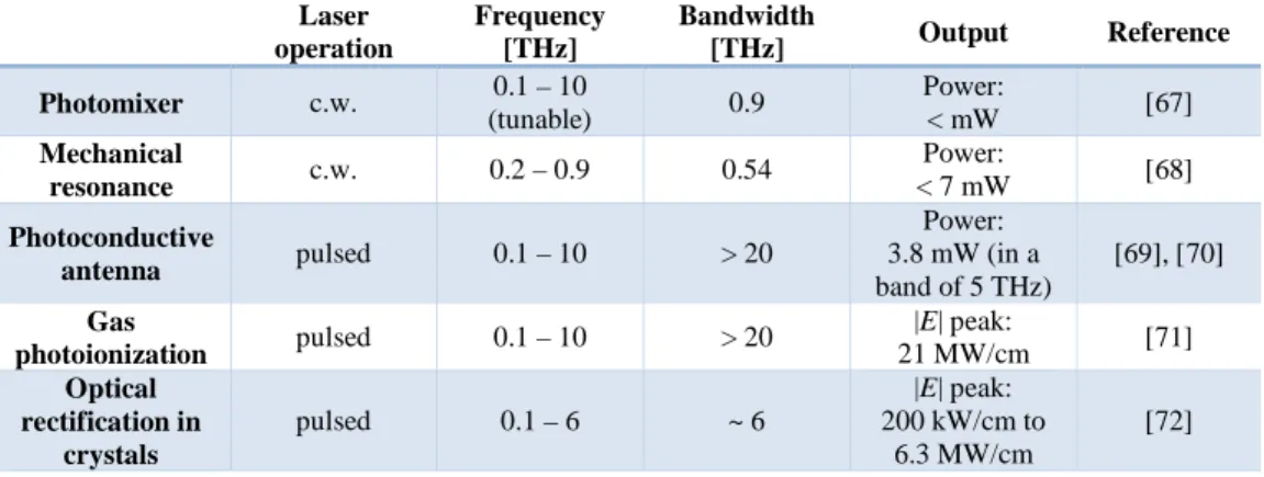
Optical and near-IR lasers generating THz radiation by optical pumping are the most employed sources, especially for spectroscopy applications, because they do not need cooling and are enough compact to be portable. They can operate in pulsed or continuous wave mode (c.w.). A comparison of properties for some examples of these two operational modes can be found in Table 2.

Table 2 Comparison between some techniques employing optical and near-infrared lasers for generating

THz radiation by optical pumping.

Laser operation Frequency [THz] Bandwidth [THz] Output Reference Photomixer c.w. 0.1 – 10 (tunable) 0.9 Power: < mW [67] Mechanical resonance c.w. 0.2 – 0.9 0.54 Power: < 7 mW [68] Photoconductive antenna pulsed 0.1 – 10 > 20 Power: 3.8 mW (in a band of 5 THz) [69], [70] Gas photoionization pulsed 0.1 – 10 > 20 |E| peak: 21 MW/cm [71] Optical rectification in crystals pulsed 0.1 – 6 ~ 6 |E| peak: 200 kW/cm to 6.3 MW/cm [72]

(43)

9

Continuous lasers can be mixed for generating radiation in the THz band. This kind of sources are called photomixers and generate THz radiation by optical heterodyning [73]. They have a better spectral resolution than pulsed emitters and output powers in the order of milliwatts [74]. Moreover, they can be employed as sources for spectroscopy as well as for THz communications. However, they operate in narrowband and have limited tuning ranges.

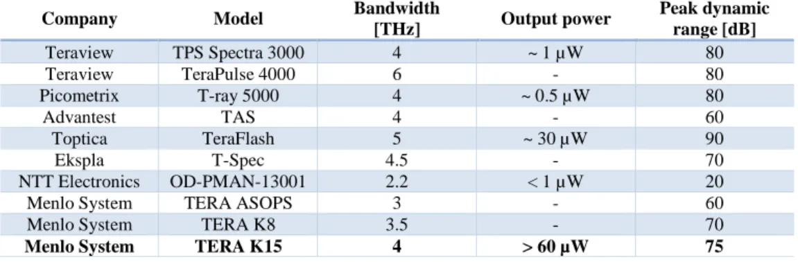
Pulsed lasers are employed for exciting a photoconductive switch or antenna. They are also able to produce THz by three different mechanism: (i) gas photoionization, (ii) optical rectification in a non-linear crystal, and (iii) drift or diffusion of transient currents in a semiconductor with high charge mobility [75]. Pulsed lasers generation technology is the base of time-domain spectroscopy (TDS). The configuration of a typical TDS set-up with photoconductive antennas will be described in detail in chapter V. In Table 3, properties of several commercial available TDS with photoconductive antennas are compared.

Table 3 Commercially available THz time-domain spectrometers generating THz radiation by

photoconductive antennas (readapted from [76]).

Company Model Bandwidth

[THz] Output power Peak dynamic range [dB] Teraview TPS Spectra 3000 4 ~ 1 µW 80 Teraview TeraPulse 4000 6 - 80 Picometrix T-ray 5000 4 ~ 0.5 µW 80 Advantest TAS 4 - 60 Toptica TeraFlash 5 ~ 30 µW 90 Ekspla T-Spec 4.5 - 70 NTT Electronics OD-PMAN-13001 2.2 < 1 µW 20

Menlo System TERA ASOPS 3 - 60

Menlo System TERA K8 3.5 - 70

Menlo System TERA K15 4 > 60 µW 75

3. Terahertz detectors

Unlike detectors for visible and infrared radiation, detectors for THz waves have not reached the quantum limit yet [77]. In fact, detector characteristics are not limited by noise due to photons, except for measurements at some frequencies or at sub-kelvin temperatures [78].

The performance of a THz set-up is influenced by sensitivity, responsivity, and frame rate of its detector(s). The sensitivity is expressed by a figure of merit, the noise

(44)

10

equivalent power (NEP). NEP is defined as the incident power that gives a signal-to-noise ratio (SNR) equal to one in an output bandwidth of 1 Hz. Low values of NEP express a high sensitivity. Mathematically [79]:

NEP = CD

EF (I.1)

where, vn is the noise voltage spectral density, i.e. the noise power per unit of bandwidth, and Rv is the responsivity, i.e. the input-output gain of the detector.

For an imaging detector, constituted by a certain number of pixels, a NEPcamera is usually indicated, where: NEP = NEP_{GH3 H}⁄√bandwidth. NEP is expressed in W/√Hz. The NEPcamera is expressed in W and can be computed as [79]:

NEPGH3 H= _∑_\]]\^CDWXD_Z_[ (I.2)

where Pin is the total incident THz power and Vi is the signal of the ith pixel of the

detector array.

Table 4 Commercial available detectors for THz radiation [25]. Frequency [THz] Responsivity [V/W] NEP or NEPcamera Frame rate or response time Number of pixels Company Schottky barrier diode 0.11 – 0.17 2000 13.2 pW/Hz½ 42 ns Single detector VDI Photoconductive antenna 0.1 – 4.0 - - - Single detector EKSPLA Photoconductive folded dipole antenna 0.6 – 1.0 800 66 pW/Hz½ - Single detector STM Photoconductive antenna 0.3 – 4.5 - - - Single detector Menlo System FET array 0.7 – 1.1 115·10 3 12 nW 25 Hz 32x32 STM Bolometer 4.25 - 24.7 pW 50 Hz 384x288 INO Golay cell 0.2 – 20 10·103 10 nW/Hz½ 25 ms Single detector Microtech Micro-bolometer 1.0 – 7.0 - < 100 pW 30 Hz 320x240 NEC LiTaO3 pyroelectric 0.1 – 300 - 96 nW 50 Hz 320x320 Ophir photonics Pyroelectric 0.3 1.0 3.010 18.3·103 440 pW/Hz½ 10 Hz Single detector QMC α-Si micro-bolometer 2.4 14·10 6 30 pW - 320x240 CEA-Leti VOx micro-bolometer 2.8 200·10 3 35 pW 30 Hz 160x120 Infrared Systems VOx micro-bolometer 3.1 - 280 pW 16 ms

(each pixel) 640x480 NEC

Antenna QW

(45)

11

In Table 4, parameters of several commercially available THz detectors are compared. According to The 2017 terahertz science and technology roadmap [25], detectors based on CMOS technology, such as photoconductive antennas and FET arrays, are the most promising tools for THz sensing and imaging. In fact, they are suitable for miniaturization and integration in compact devices and are able to operate at room temperature. However, improvements are needed for increasing responsivity, sensitivity and response times, as well as, in imaging, the number of available pixels [25]: “Future expectations for terahertz imaging systems include video rate imaging (at least 25 fps) at VGA resolution. Further into the future, HD format will be the normal expectation for any imaging system. Image resolution (as opposed to display resolution), noise and dynamic range are all expected to improve. These improvements will rely on advancement in source, detector and optical/system design technology. Specifically, compact, room temperature terahertz sources in the region of 10 mW average power are essential in order to enable stand-off imaging at distances greater than 1 m. Such sources when coupled with a Si CMOS FPA would render a low-cost THz camera (we estimate < US$ 5000 per unit) that could find wide spread use in applications such as stand-off detection of hidden objects and non-invasive medical (e.g. oncology) and dental diagnostics.”

It means that the development of THz detection tools cannot ignore a progress of the whole THz components technology, included not only sources and detectors, but passive THz devices too, as discussed in the next section.

4. Terahertz passive components

Generally, when the availability of high power is fundamental for a specific application, quasi-optical devices are preferred to guided-wave structures. For example, in a commercially available metallic rectangular waveguide (WG) losses are equal to 1 dB/cm at 1 THz (Virginia Diodes VM250 (WR-1.0) [80]). In fact, at microwaves, metals behave as perfect conductors, while they are lossy at THz. Additionally, most of dielectrics extremely transparent at optical frequencies absorb THz waves (compare Ch. II Sec. 5). Guided structures, however, offer several