Università degli Studi di Ferrara
DOTTORATO DI RICERCA IN
SCIENZE DELLA TERRA
CICLO
XXV
COORDINATORE Prof. Luigi Beccaluva
Evaluation of natural and present subsidence in the
northeastern coast of the Caspian Sea
Settore Scientifico Disciplinare GEO/04
Tutore Interno Prof. Simeoni Umberto
___________________________
Dottorando Tutori Esterni
Dott. Magagnini Luca PhD. Ulazzi Elisa
_____________________________ __________________________
Prof. Teatini Pietro
__________________________ Anni 2010/2012
TABLE OF CONTENT
1. ABSTRACT ... 1
2. GOAL, OBJECTIVES, METHODOLOGY AND LIMITATIONS ... 7
3. GEO-HYDROGEOLOGICAL RECONSTRUCTION ... 17
3.1 Geology, Tectonic And Seismicity ...17
3.1.1 Brief description of main geological features in the Caspian area ... 17
3.1.2 The North Caspian Basin Structure ... 23
3.1.3 The North Ustyurt Basin Structure ... 68
3.2 Stratigraphy ...75
3.2.1 North and West Basin Margin ... 77
3.2.2 East-Southeast Basin Margin ... 79
3.2.3 South Basin Margin ... 81
3.2.4 Details on Zones B and C ... 85
3.3 Details About Salt Dome Structures ...88
3.3.1 Permian Deposition, Salt Formation, and Movements ... 90
3.3.2 Triassic Deposition and Salt Movements ... 91
3.3.3 Jurassic Deposition and Salt Movements (Mainly Extrusion and Overhangs) ... 94
3.3.4 Jurassic–Paleogene Deposition and Polygonal Faults ... 98
3.3.5 Cenozoic Deposition ... 103
3.4 Soils Distribution And Characterisation ... 107
3.4.1 Spatial distribution of soil features in Zone B (Northern Area, from Atyrau City to the Emba River valley) ... 109
3.4.2 Spatial distribution of soil features in Zone C (North – Eastern Area, from the basin of the Emba River to the Mertvyy Kultuk Bay) ... 114
3.4.3 Spatial distribution of soil features in Zone D (Southern Area, Northern Shoreline of Buzachi Peninsula) ... 118
3.5 Hydrogeological Setting ... 124
3.5.1 Spatial distribution of hydrogeological features in Zone B (from Atyrau City to the Emba River valley) ... 125
3.5.2 Spatial distribution of hydrogeological features in Zone C (from the basin of the
Emba River to the Mertvyy Kultuk Bay) ... 128
3.5.3 Spatial distribution of hydrogeological features in Zone D (Northern Shoreline of Buzachi Peninsula) ... 130
3.5.4 Hydrogeology of the Tyub-Karagan Peninsula ... 133
3.5.5 Future Use of the Underground Waters ... 133
3.6 Oil&Gas Resources ... 138
3.6.1 Description of thePrecaspian basin petroleum system... 138
3.6.2 Oil&Gas Resources of the North Ustyurt Basin ... 143
4. EVALUATION OF NATURAL AND PRESENT SUBSIDENCE ...147
4.1 Rock Compressibility ... 147
4.1.1 Definitions ... 147
4.1.2 Measurements of rock compressibility ... 151
4.1.3 Pore compressibility calculated by traveltime log ... 156
4.2 Natural Susidence Calculation Through Numerical Modeling ... 165
4.2.1 Preliminary Analysis Of Natural Subsidence Numerical Models ... 165
4.2.2 Synthetic overview of existing models ... 166
4.2.3 The Natsub code ... 172
4.2.4 The Basin code ... 189
4.2.5 Models application and results ... 200
4.2.6 General discussion of NATSUB and BASIN output ... 255
4.3 Evaluation Of Present Subsidence By Sar Interferometry ... 257
4.3.1 Principles of Interferometric SAR technique ... 257
4.3.2 SAR resolution: cell projection on the ground ... 262
4.3.3 Applications and limits... 265
4.3.4 Innovative aspects of InSAR application to the study area ... 277
4.3.5 Analysis and interpretation of SBAS results ... 304
4.3.6 Preliminary application of IPTA ... 325
4.3.7 Comparison of achieved results with the northern Adriatic coastland case study ... 335
5. CALCULATED AND MEASURED RESULTS COMPARISON AND CONCLUSION ...347
6. SWOT ANALYSIS ...349
7. FUTURE SCENARIO ESTIMATION ...351
8. MONITORING PLAN ...353
8.1 Spatial and temporal distribution of radar images acquisition for SBAS monitoring analysis within frames Z1, Z2 and Z3 ... 353
8.2 Integration of monitoring plan with artificial Persistent Scatters and fix GPS
stations ... 353
8.3 Best solution for fix GPS installation ... 357
9. PROPOSED NEXT ACTIVITIES ... 361
9.1 Present subsidence monitoring along the whole Kazakh coastal area ... 361
9.2 Creation of a Digital Elevation Model ... 363
9.3 InSAR analysis on production islands ... 366
10. REFERENCES ... 367
LIST OF FIGURES
Figure 1: Landscapes within Frame Z1, along the Ural river vegetated belt and
Eskene area. ...10 Figure 2: Landscapes within Frame Z3, Buzachi peninsula...11 Figure 3: Study area subdivision ...11 Figure 4: Links between the geo-hydrogeological reconstruction and activities carried
out during the analysis of present subsidence. ...13 Figure 5: Tectonic scheme of the North Caspian Region, after “A. P. Afanasenkov et.
al., 2008” ...19 Figure 6: Petroleum system and assessment units of North Caspian Basin. After G.
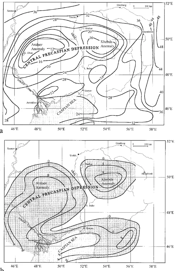
F. Ulmishek, 2003”. ...23 Figure 7: Structural map of the North Caspian Basin, after “G. F. Ulmishek, 2003”. ...26 Figure 8: Isobathic maps of Precaspian Basin at the level of main reflectors, isolines
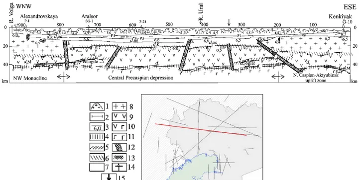
in km, after “Yu.A. Volozh et al., 2003”. ...28 Figure 9: Geological –geophysical crustal section Volgograd –Chelkar, after “Volozh
et al., 2003”. ...29 Figure 10: Palinspastic reconstruction along a profile on the east Precaspian margin,
line Ural River –Izembet (Urals), after “Volozh et al., 2003”. ...30 Figure 11: Reconstruction of evolution of the Precaspian Basin along a N–S line after
“Brunet et al., 1999”. Layers are reconstituted without the movements of
salt. ...31 Figure 12: Palaeogeological reconstruction across profile Karaton–Tengiz–Yuzhnaya,
southeast Precaspian margin, after “Volozh et al., 2003”. ...32 Figure 13: Geodynamic reconstructions of Riphean–Vendian history, after “Volozh et
al., 2003”. ...34 Figure 14: Riphean– Early Palaeozoic geodynamic reconstruction along an East–West
section demonstrating eclogites emplacement, after “Volozh et al., 2003”. ...35 Figure 15: Map of the crustal thickness without HVL (a) and thickness of the HVL (b),
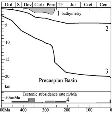
after “Brunet et al., 1999”. ...38 Figure 16: Subsidence curves in the centre of the Precaspian Basin, after “Brunet et
al., 1999”. ...42 Figure 17: Stratigraphical site of seismic reflector P3, by Akhmetshina et al., 1993
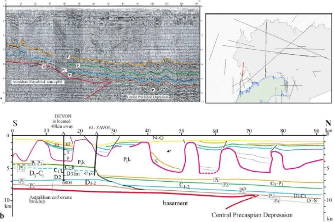
Figure 18: North– south section on the southwest Astrakhan margin of the Precaspian
Basin, after “Volozh et al. 2003”. ... 45 Figure 19: Structural and tectonic map showing consolidated crust in the Caspian
region, after “Volozh et al., 2009”. ... 48 Figure 20: Geologic-geophysical section across the South Emba uplift (b) and a
fragment of time section (a) showing the morphology of tectonic dislocations within the South Emba regional fault, after “Volozh et al.,
1999”. ... 49 Figure 21: Gross depositional environment map of the Ordovician, after “Volozh and
Parasyna, 2008”. ... 50 Figure 22: Geologic section through the Tsimlyansk line across the Karpinskiy Range,
after “Volozh et al., 1999”. ... 51 Figure 23: Paleotectonic reconstructions across the Tsimlyansk line illustrating the
major tectonic events that result in the development of the Sarmat–Turkyr
rift system, after “Volozh et al., 2009”. ... 52 Figure 24: Palinspastic reconstruction of consolidated crust of the Paleozoic East
European continent at the beginning of the Kungurian, after “Volozh and
Parasyna, 2008”. ... 53 Figure 25: Relationship between structural geometry of different sequences of the
sedimentary cover, North Caspian salt dome region,after “Volozh et al.,
2009”. ... 55 Figure 26: Cross-section across the Ural foredeep, after “Volozh et al., 2009”... 56 Figure 27: Fragment of time section through a regional line across junction zone
between the Ural foredeep and East Orenburg arch, after “Volozh et al.,
2009”. ... 56 Figure 28: Paleozoic (presalt) petroleum potential, after “Volozh et al., 2009”... 59 Figure 29: Diagram of amplitudes of recent tectonic movements in the Caspian and
Turanskaya Platform regions, after “KDCP, 2002”. ... 62 Figure 30: Diagram of recent (active) faults in the Caspian and Turanskaya Platform
regions, after KDCP, 2002. ... 65 Figure 31: Earthquakes of the North Caspian Region, after “Granherne, 2006”. ... 67 Figure 32: Petroleum system and assessment units of the North Ustyurt basin, after
“Ulmishek, 2003”. ... 69 Figure 33: Principal structural unit of the North Ustyurt basin, after “Ulmishek, 2003”. ... 70 Figure 34: Generalized structure of Buzachi arch and adjacent areas, after “G.F.
Ulmishek, 2003”. ... 72 Figure 35: Cross-section through north basin margin. Located in the westernmost
portion of the northern margin. After “Ulmishek, 2003” and Cross section
through Karachaganak carbonate build-up, after “Ulmishek, 2003”. ... 78 Figure 36: Cross section through east basin margin, after “Ulmishek, 2003”. ... 80 Figure 37: Carbonate build-ups of northern Caspian Sea. Scale approximate. After
“Ulmishek, 2003”. ... 81 Figure 38: Cross section of Karaton-Tengiz zone, after “Ulmishek, 2003”. ... 83
Figure 39: Cross section of Astrakhan arch, after “Ulmishek, 2003”. ...84 Figure 40: Well section stratigraphic correlation in Caspian Sea and coastal zones,
after “GAS, 2007”. ...85 Figure 41: Synthetic column in the centre of the Precaspian basin, showing the
thickness of sediments, paleo water depths, ages and main seismic
horizons, with velocities and density. ...86 Figure 42: Schematic cross-section NW-SE across Tengiz-Karaton Platform, after
“Max Petroleum, 2010”...87 Figure 43: Summary of the typical stratigraphy in Zone C. ...87 Figure 44: Historical map of salt domes in Southern Precaspian Basin, after “Sanders,
1939”. ...88 Figure 45: Historical dome cross-section, after “Sanders, 1939”. ...89 Figure 46: Salt structures in the Precaspian basin from the Triassic to the
EarlyJurassic, after “Volozh et al., 2003”. ...91 Figure 47: Map of Precaspian basin showing current shapes of salt structures, after
“Volozh et al., 2003”. ...92 Figure 48: Seismic profile (located in Emba River Valley) and restoration to stated
times. Dotted line along right-hand end of restored profiles indicates
changing profile length by area balancing. ...94 Figure 49: Summary of sedimentation and halokinesis in the Precaspian basin.
Regions a1–b5 are identified in Figure 47. ...97 Figure 50: The sheet of allochthonous Kungurian salt at Kum (Kazakh area of the
Volga mouth) was extruded in the Late Jurassic and began to upbuild
during the Paleogene, after “Volozh et al., 2003”. ...98 Figure 51: The Kotyrtas North oil field (located on North Emba River Valley) is trapped
above a sheet of allochthonous Kungurian salt extruded in the Middle
Triassic, after “Volozh et al., 2003”. ... 101 Figure 52: A sheet of allochthonous Kungurian (±Kazanian salt) extruded in the Middle
to Late Triassic trapped the Novobogatinsk oil field (located near Atyrau),
after “Volozh et al., 2003”. ... 102 Figure 53: Maps of part of the southern Precaspian basin showing normal faults
off-setting base Cretaceous, after “Volozh et al., 2003”. ... 103 Figure 54: Structural map of the Precaspian basin in Pliocene times illustrating
incisions and canyons eroded through Cretaceous platform sediments bythe paleo-Volga and paleo-Amu-Dariya rivers draining into the South Caspian lake having a surface about 1 km below ocean level, after “Volozh
et al., 2003”. ... 105 Figure 55: Map of soils distribution between Atyrau City and Emba River Valley, after
“Mo Energy and Mineral resources et al., 2001”. ... 112 Figure 56: Map of soils distribution between Emba River basin and Mertvyy Kultuk
Bay, after “Mo Energy and Mineral resources et al., 2001”. ... 116 Figure 57: Map of soils distribution in the Northern shoreline of the Buzachi Peninsula,
Figure 58: Groundwater depths in Zone B ... 126
Figure 59: Groundwater depths in Zone C ... 129
Figure 60: Groundwater depths in Zone D ... 132
Figure 61: Mineral and iodine-bromine underground waters in the study area (green circles) ... 135
Figure 62: Events chart of North Caspian Total Petroleum System, after “Ulmishek, 2003”. ... 140
Figure 63: Sketch of an extensometric apparatus using a string of solid pipes... 153
Figure 64: Radioactive marker technique for measuring the compaction of deep formations. ... 154
Figure 65: Evaluation of bottom velocity and land subsidence over the last three centuries, projected until 2100 in the Emilia-Romagna coast, using NATSUB, after “Gambolati et al., 1999.” ... 167
Figure 66: Three main conceptual blocks of the Galo model, after (Makhous et al, 1997). ... 169
Figure 67: DeCompactionTool work flow, after “Holzel et al., 2008”. ... 170
Figure 68: Print-screen of TerraMod software. ... 171
Figure 69: The sediment column has height l(t) at time t after inception of the accretion process and rests on an impermeable basement at z=0. Seawater elevation is L. ... 175
Figure 70: Typical compression profile of a cohesive soil vs. the effective intergranular stress: a) arithmetic plot and b) semilogarithmic plot. ... 180
Figure 71: Log-log graphic of the whole compressibility dataset. ... 207
Figure 72: Porosity n vs. depth z at Test 1 well, for different compressional trends. ... 211
Figure 73: Porosity n vs. depth z at Test 2 well, for different compressional trends. ... 212
Figure 74: Porosity n vs. depth z at Test 3 well, for different compressional trends. ... 212
Figure 75: Porosity n vs. depth z at Test 4 well, for different compressional trends. ... 213
Figure 76: Porosity n vs. depth z at Test 5 well, for different compressional trends. ... 213
Figure 77: Sedimentation rate (Sed.rate) and settling velocity (Bott.vel.) vs. geological time (high trend). ... 229
Figure 78: Sedimentation rate (Sed.rate) and settling velocity (Bott.vel.) vs. geological time (mean trend). ... 229
Figure 79: Sedimentation rate (Sed.rate) and settling velocity (Bott.vel.) vs. geological time (low trend) ... 229
Figure 80: AK1 Sedimentary column depths comparison, at selected time steps (high, mean and low trends... 229
Figure 81: Sedimentary column compaction vs. time. ... 229
Figure 82: Pore pressure vs. depth. ... 229
Figure 83: Pore pressure vs. time. ... 229
Figure 84: Sedimentation rate (Sed. rate) and settling velocity (Bott.vel.) vs. geological time (high trend). ... 231
Figure 85: Sedimentation rate (Sed. rate) and settling velocity (Bott.vel.) vs. geological
time (mean trend). ... 231
Figure 86: Sedimentation rate (Sed. rate) and settling velocity (Bott.vel.) vs. geological time (low trend). ... 231
Figure 87: Sedimentary column depths comparison, at selected time steps. ... 231
Figure 88: Sedimentary column compaction vs. time. ... 231
Figure 89: Pore pressure vs. depth. ... 231
Figure 90: Pore pressure vs. time ... 231
Figure 91: Sedimentation rate (Sed.rate) and settling velocity (Bott.vel.) vs. geological time (high trend). ... 233
Figure 92: Sedimentation rate (Sed.rate) and settling velocity (Bott.vel.) vs. geological time (mean trend). ... 233
Figure 93: Sedimentation rate (Sed.rate) and settling velocity (Bott.vel.) vs. geological time (low trend). ... 233
Figure 94: Sedimentary column depths comparison, at selected time steps. ... 233
Figure 95: Sedimentary column compaction vs. time ... 233
Figure 96: Pore pressure vs. depth. ... 233
Figure 97: Pore pressure vs. time. ... 233
Figure 98: Sedimentation rate (Sed.rate) and settling velocity (Bott.vel.) vs. geological time (high trend). ... 235
Figure 99: Sedimentation rate (Sed.rate) and settling velocity (Bott.vel.) vs. geological time (mean trend). ... 235
Figure 100: Sedimentation rate (Sed.rate) and settling velocity (Bott.vel.) vs. geological time (low trend). ... 235
Figure 101: Sedimentary column depths comparison, at selected time steps. ... 235
Figure 102: Sedimentary column compaction vs. time ... 235
Figure 103: Pore pressure vs. depth. ... 235
Figure 104: Pore pressure vs. time. ... 235
Figure 105: Sedimentation rate (Sed.rate) and settling velocity (Bott.vel.) vs. geological time (high trend). ... 237
Figure 106: Sedimentation rate (Sed.rate) and settling velocity (Bott.vel.) vs. geological time (mean trend). ... 237
Figure 107: Sedimentation rate (Sed.rate) and settling velocity (Bott.vel.) vs. geological time (low trend). ... 237
Figure 108: Sedimentary column depths comparison, at selected time steps. ... 237
Figure 109: Sedimentary column compaction vs. time ... 237
Figure 110: Pore pressure vs. depth. ... 237
Figure 111: Pore pressure vs. time. ... 237
Figure 112: Position of numerical simulation 2D section. ... 240
Figure 113: Chronostratigraphy simulated through BASIN model (Simulation 1) and comparison with schematic cross-section elaborated by Max Petroleum (2008). ... 244
Figure 114: Simulation’s mesh at different time steps (Late Devonian, Serpukhovian-Bashkirian boundary, Triassic-Jurassic boundary, Early Cretaceous)
(Simulation 1). ... 245
Figure 115: Porosity at different time steps (Late Devonian, Serpukhovian-Bashkirian boundary, Triassic-Jurassic boundary, Early Cretaceous) (Simulation 1). ... 246
Figure 116: Specific storage at different time steps (Late Devonian, Serpukhovian-Bashkirian boundary, Triassic-Jurassic boundary, Early Cretaceous) (Simulation 1). ... 247
Figure 117: Hydraulic conductivity at different time steps (Late Devonian, Serpukhovian-Bashkirian boundary, Triassic-Jurassic boundary, Early Cretaceous) (Simulation 1). ... 248
Figure 118: Consolidational settling rate at different time steps (Late Devonian, Serpukhovian-Bashkirian boundary, Triassic-Jurassic boundary, Early Cretaceous) (Simulation 1). ... 249
Figure 119: Simulation’s mesh at different time steps (Late Devonian, Serpukhovian-Bashkirian boundary, Triassic-Jurassic boundary, Early Cretaceous) (Simulation 2). ... 250
Figure 120: Porosity at different time steps (Late Devonian, Serpukhovian-Bashkirian boundary, Triassic-Jurassic boundary, Early Cretaceous) (Simulation 2). ... 251
Figure 121: Specific storage at different time steps (Late Devonian, Serpukhovian-Bashkirian boundary, Triassic-Jurassic boundary, Early Cretaceous) (Simulation 2). ... 252
Figure 122: Hydraulic conductivity at different time steps (Late Devonian, Serpukhovian-Bashkirian boundary, Triassic-Jurassic boundary, Early Cretaceous) (Simulation 2). ... 253
Figure 123: Consolidational settling rate at different time steps (Late Devonian, Serpukhovian-Bashkirian boundary, Triassic-Jurassic boundary, Early Cretaceous) (Simulation 2). ... 254
Figure 124: SAR system from a satellite (Ferretti et al., 2007). ... 259
Figure 125: Sinusoidal function sin φ is periodic with a 2π radian period. ... 261
Figure 126: Effect of terrain on the SAR image. ... 263
Figure 127: Layover and shadow effects. ... 264
Figure 128: ENVISAT resolution cell dimension in ground range as a function of the terrain slope. The vertical dotted line indicates the incidence angle relative to a flat horizontal terrain (23°) (Ferretti et al., 2007). ... 265
Figure 129: Geometry of a satellite interferometric SAR system. ... 266
Figure 130: Geometric parameters of a satellite interferometric SAR system (Ferretti et al., 2007)... 267
Figure 131: Interferometric phase dispersion (degrees) as a function of the coherence for varying numbers of looks (NL) (Ferretti et al., 2007). ... 272
Figure 132: Interferometric phase dispersion exact values (blue curves) and approximated ones (red curves) (Ferretti et al., 2007)... 272
Figure 134: Frames of SBAS application in the area of interest. ... 279
Figure 135: Images focused on Frame Z1. ... 282
Figure 136: Images focused on Frame Z2. ... 283
Figure 137: Images focused on Frame Z3. ... 284
Figure 138: Topographic reference of the study area based on SRTM. ... 285
Figure 139: Temporal and spatial baseline of frame Z1. ... 286
Figure 140: Temporal and spatial baseline of frame Z2. ... 287
Figure 141: Temporal and spatial baseline of frame Z3. ... 287
Figure 142: Possible interferograms with baselines shorter than 200 m in frame Z1. ... 288
Figure 143: Possible interferograms with baselines shorter than 200 m in frame Z2. ... 289
Figure 144: Possible interferograms with baselines shorter than 200 m in frame Z3. ... 290
Figure 145: Location of the reference point (green triangle) in each frame... 291
Figure 146: Interferograms considered after phase unwrapping in frame Z1. ... 299
Figure 147: Interferograms considered after phase unwrapping in frame Z2. ... 300
Figure 148: Interferograms considered after phase unwrapping in frame Z3. ... 301
Figure 149: Interferograms considered after multi-baseline interferometry analysis in frame Z1. ... 302
Figure 150: Interferograms considered after multi-baseline interferometry analysis in frame Z2. ... 302
Figure 151: Interferograms considered after multi-baseline interferometry analysis in frame Z3. ... 303
Figure 152: Results of SBAS analysis in frame Z1. ... 305
Figure 153: Detail of SBAS analysis within frame Z1. ... 307
Figure 154: Results of SBAS analysis in frame Z2. ... 313
Figure 155: Uplifts along the coastal area. ... 314
Figure 156: Results of SBAS analysis in frame Z3. ... 320
Figure 157: Identification of candidate persistent scatterers in frame Z1. ... 326
Figure 158: Identification of candidate persistent scatterers in frame Z2. ... 327
Figure 159: Identification of candidate persistent scatterers in frame Z3. ... 328
Figure 160: Results of IPTA before outlayers filtering. ... 329
Figure 161: Example of local displacements in a zone of Atyrau (light blue dots: rates value between ±2 mm/y; yellow dots: rates value between -2 and -8 mm/y). ... 330
Figure 162: Location of the persistent scatterers removed from the regional investigation. ... 331
Figure 163: Displacement map for the frame Z1 obtained by IPTA after filtering out the measurements affected by a site-specific displacement trend. ... 332
Figure 164: Comparison between IPTA (left) and SBAS (right) on the whole frame Z1 and in correspondence to Atyrau. ... 333
Figure 165: Differences between IPTA and SBAS analysis. ... 334
Figure 166: Digital elevation model (DEM) of the northern Adriatic region obtained from SRTM data. ... 336
Figure 167: Relative sea level rise (RSLR) at Venice and Ravenna over the period
1896–2007. ... 336
Figure 168: Recent natural land subsidence in the northern Adriatic coastal area (after Gambolati and Teatini 1998). ... 337
Figure 169: Vertical displacement rates (mm/year) in the Venetian region obtained by the SIMS over the decade 1992–2002. ... 340
Figure 170: Vertical displacement rates (mm/year) in the Venetian coastland obtained by IPTA of ENVISAT scenes acquired between 2003 and 2007. ... 341
Figure 171: Map of the cumulative displacements (cm) occurring from 1992 to 2007 in the Venetian coastland as obtained by the integration of ERS-1/2 and ENVISAT IPTA results. Green dots position of the IGM34 (IRMA54) leveling benchmarks used for the validation of the IPTA outcomes. ... 342
Figure 172: Comparison between leveling and IPTA results along the IGM34 (IRMA54) line. ... 342
Figure 173: Parallelisms between two different study areas... 344
Figure 174: Reached detail of SAR based measured at Venice (Teatini et al., 2007). ... 345
Figure 175: Example of sedimentation rate and settling velocity during future scenario, well Test 3. ... 351
Figure 176: Example of depth (or thickness) of the sedimentary column during future scenario, well Test 3 ... 352
Figure 177: Identified PT in frame Z1 ... 354
Figure 178: Identified PT in frame Z2 ... 354
Figure 179: Identified PT in frame Z3 ... 355
Figure 180: Integration between natural and artificial PTs ... 356
Figure 181: Location of the GPS stations in international GPS networks around the Caspian Sea (after SOPAC archives, http://sopac.ucsd.edu/sites/)... 357
Figure 182: Possible GPS location (red circle) within frame Z1 ... 358
Figure 183: Possible GPS location (red circle) within frame Z2 ... 358
Figure 184: Possible GPS location (red circle) within frame Z3 ... 359
Figure 185: Snapshot of ESA imagery catalogue ... 361
Figure 186: RADARSAT-1 tracks covering the north-eastern Caspian. The red "squares" represent the three frames selected from the ENVISAT-ASAR archive. ... 362
Figure 187: Preliminary selection of RADARSAT-1 frames (in blue) for the DInSAR analysis. ... 362
Figure 188: DEM generation in the eastern part of the Volga Delta: step of elaboration. ... 365
Figure 189: Distances between artificial islands at Kashagan area ... 366
LIST OF TABLES
Table 1: Advantages and disadvantages of applied methodologies. ...13
Table 2: Geodynamic events linked to sedimentary environment in the PCB, after “Volozh et al., 2003”. ...37
Table 3: Regional quaternary stratigraphy. ... 107
Table 4: Preliminary evaluation of Numerical models. ... 166
Table 5: Main logs used for this study. ... 200
Table 6: Mean values of e0 vs. z0 founded in geotechnical reports and values assumed during the model application for z0=20 m. ... 210
Table 7: Depth of available sonic logs... 216
Table 8: Present thickness of the layering sequence at Test 1 as compared to the uncompacted thickness bi. ... 217
Table 9: Present thickness of the layering sequence at Test 2 as compared to the uncompacted thickness bi. ... 219
Table 10: Present thickness of the layering sequence at Test 3 as compared to the uncompacted thickness bi. ... 221
Table 11: Present thickness of the layering sequence at Test 4 as compared to the uncompacted thickness bi. ... 223
Table 12: Present thickness of the layering sequence at Test 5 as compared to the uncompacted thickness bi. ... 225
Table 13: Comparison between present total thicknesses and uncompactedones. ... 227
Table 14: Results sheet description. ... 228
Table 15: Dates and orbits of acquisition. ... 279
Table 16: List of interferograms considered after phase unwrapping. ... 292
Table 17: Displacements versus time for a few sites selected within the Z1 frame. ... 308
Table 18: Displacements versus time for a few sites selected within the frame Z2. ... 316
Table 19: Displacements versus time for a few sites selected within the frame Z3. ... 322
Table 20: Natural and present SWOT analysis ... 349
Table 21: Summary of SRTM performance. All quantities represent 90% errors in meters. ... 363
ACRONYMS
ATM: Atmospheric (referred to DInsar analysis); BH: Borehole;
BoD: Basis of Design;
BTOE: Billion Tons of Oil Equivalent; CAL: Caliper
CMB: Crust/Mantle Boundary;
CPD: Central Precaspian Depression; CPT: Cone Penetration Testing; DEM: Digital Elevation Model;
DInSAR:Differential Interferometric Synthetic Aperture Radar; ESA: European Space Agency;
GDB: Geodatabase;
GIS: Geographic Information System; GOR: Gas Oil Ratio;
GPS: Global Positioning System;
ICZM: Integrated Coastal Zone Management; InSAR: Interferometric Synthetic Aperture Radar; IPTA: Interferometric Point Target Analysis; LAS: Log Ascii Standard
LOS: Line of Sight;
LS: Last square solution;
NCB: North Caspian Basin; NPHI: Neutron porosity; NL: Number of looks;
PSI: Persistent Scatterer Interferometry; PCB: Precaspian Basin;
RHOB: Bulk density;
SAR: Synthetic Aperture Radar; SBAS: Small Baseline Subset TPF: Temporal Phase Filtered TPS: Total Petroleum System;
1. ABSTRACT
The main goal of the study is to test different methodologies helpful for the definition of natural and present subsidence along coastal area. Specifically, tests were carried out on the Kazakh coastal area (northeastern part of the Caspian Sea coast).
Specific objectives include:
• the reconstruction of the geological assets of the projects area;
• the definition of processes that influence the subsidence under specific geological conditions;
• the calculation, through numerical models application (both 1D – NATUB and 2D - BASIN), of natural subsidence;
• the detection of present ground vertical movements through Synthetic Aperture Radar Interferometry (InSAR), from 2003 to 2009.
Collected data was derived from international literature (especially for the basin-scale) and from O&G companies reports and surveys, and considering several geological disciplines (stratigraphy, geodynamics, hydrogeology etc.).
Integration of data and the reconstruction of the geological framework of the area have been developed at different scales:
basin-scale: regional geology and geodynamic evolution of the Precaspian Basin and the North Ustyurt Basin;
local scale: four subareas of the northern part of the Caspian Sea have been identified. For each subarea, when data is available the study focuses on the complexity and variability of the area; the stratigraphic complexity is determined by several kilometres of clastic and carbonatic sediments interrupted by 4 km salt layer, a distribution of soil features (with geotechnical properties) linked to the interaction of fluvial and marine dynamics, prevalence of saline waters in a multistage aquifer system, and the presence of oil and gas reservoirs.
The realization of a datasets (stratigraphy, geochronology, compressibility of different sedimentary layers, etc.) required by activities foreseen during the analysis of natural subsidence has been exhaustively fulfil.
This data has been used as input during the mono- and bi- dimensional numerical simulation of natural subsidence on 5 different locations.
Collected data provided also information required for the interpretation of the present subsidence detected by InSAR analysis; the application of two different InSAR techniques ((Small BAseline Substet and Interferometric Poin Target Analysis), never tested in coastal environments similar to this one, allowed to measure vertical land movements at local scale; sometimes lack of data on top on that linked to salt dome characteristics does not permit a detailed correlation between vertical movements detected and their geological causes.
NATSUB and BASIN models outputs underline the stable behaviour of the area and the absence of clear subsidential phenomena.
In the southern margin of the Precaspian basin, the limited depth of elder drilled strata (carbonates of Devonian period) reveals that the basin was filled with very low rates of sedimentation and NATSUB shows that consolidational processes were coeval with sedimentational ones. Therefore, subsidential processes do not affect the deep and ancient rocks, and BASIN application shows that the consolidation involves only shallow sedimentary layers.
DInSAR analysis, applied on three 100x100 km frames and based on ENVISAT images acquired between 2003 and 2009, confirms the calculated trend. Recorded movements for the most of the area investigated are negligible, with values comprise between ±1 mm/y.
This technique identified areas of particular interest (with values up to -6 and +5), in which movements are probably linked to salt diapirs (uplifts in correspondence to the top of the salt domes, and lowerings more marked within intra-domes areas) or coastal processes.
Results coming from two different methodologies are compared and confirm that the study area considered in present study is a stable one, with very low values of subsidence caused by sediments’ compaction.
It is important to underline that InSAR technique is suitable for detecting both wide and localised displacement linked to human activities, and during natural-present subsidence analysis some signals which would deserve further interest have been revealed also in in-land areas, even if not fully presented for confidentiality agreement.
In order to fully understand the behaviour of the sedimentary column involved in anthropic processes, deeper analysis in these area through the acquisition of newest and updated radar images could be of interest for other operators . Moreover, both achieved and new results must be linked and interpreted with information related to ongoing processes.
A monitoring plan is given, considering both applied methodologies and new solutions for results improvement.
To take advantage of applied methodologies under different point of view, a set of possible future studies linked to reservoirs development are provided.
L’obiettivo principale del presente studio è la sperimentazione di differenti metodologie utili alla definizione della subsidenza naturale e presente in zone costiere. Nello specifico, viene presa in esame la costa Kazaka (porzione nordorientale del Mar Caspio).
Obiettivi specifici dello studio includono:
• la ricostruzione degli assetti geologici locali;
• la definizione dei processi che inducono la subsidenza in condizioni specifiche;
• il calcolo, attraverso l’applicazione di modelli numerici (sia 1D – NATSUB che 2D –
BASIN) della subsidenza naturale;
• la misura dei movimenti verticali del terreno tramite la tecnologia del Radar ad Apertura
Sintetica (InSAR) per il periodo temporale 2003-2009.
I dati raccolti, provenienti sia da letteratura scientifica internazionale (specialmente quelli interessanti l’intero bacino sedimentario) che da rapporti ed indagini di differenti compagnie petrolifere operanti nell’area, riguardano diverse discipline specifiche della geologia (stratigrafia, geodinamica, idrogeologia ecc).
L’integrazione dei dati raccolti e la ricostruzione del contesto geologico dell’area sono stati sviluppati a scale di indagine differenti:
a scala di bacino: è stata considerata la geologia regionale e l’evoluzione geodinamica dei
bacini sedimentari coinvolti nello studio (Precaspian e North Ustyurt);
a scala locale: sono state dettagliate, nel tratto costiero a nordest del Mar Caspio, quattro
sotto aree. Per ciascuna di esse, lo studio approfondisce le complessità e variabilità dell’area; complessità determinata dalla presenza di sequenze kilometriche di sedimenti clastici e carbonatici interrotte da uno strato evaporitico dello spessore di circa quattro kilometri, dalla distribuzione di suoli (e conseguenti proprietà geotecniche) infuenzati dall’interazione delle dinamiche sia fluviali che costiere, dalla prevalenza di acquiferi multistrato contenenti acque con elevato tenore salino e dalla presenza di importanti giacimenti di petrolio e gas.
La realizzazione del set di dati richiesti dalle attività previste durante l’analisi della subsidenza (stratigrafia, geocronologia, compressibilità dei differenti strati) è stato completato in maniera esaustiva. Questi hanno rappresentato i dati di input durante il calcolo, tramite simulazone numerica monodimensionale e bidimensionale, della subsidenza naturale in 5 differenti posizioni. I dati raccolti hanno consentito inoltre di interpretare i valori di subsidenza presente, misurati tramite l’analisi interferometrica; l’applicazione di due differenti tecniche InSAR (Small BAseline Substet and Interferometric Poin Target Analysis), fino ad ora mai testate in ambienti costieri con caratteristiche paragonabili alla presente area di studio, hanno consentito di registrare movimenti verticali del terreno ad un livello locale, ma in alcuni casi la mancanza di
alcune informazioni (legate soprattutto al diapirismo) non ha premesso una precisa correlazione tra i tassi di spostamento misurati dall’interferometria e le relative cause geologiche.
I risultati della modellistica numerica hanno sottolineato il comportamento stabile dell’area e l’assenza di chiari fenomeni subsidenziali. Nel margine sud del bacino Precaspico, la limitata profondità degli strati più antichi perforati (carbonati del periodo Devoniano) rivela che il bacino sedimentario venne interessato da bassissimi tassi di sedimentazione e il modello monodimensionale NATSUB evidenzia che i processi di consolidazione avvennero in concomitanza con la sedimentazione. Inoltre i processi subsidenziali non coinvolgono gli strati più antichi e profondi; l’applicazione del modello bidimensionale BASIN dimostra infatti che i processi di consolidazione interessano solamente gli strati più superficiali.
L’interferometria differenziale DInSAR, applicata in tre aree della dimensione di 100x100 km sulla base di immagini ENVISAT acquisite tra il 2003 ed il 2009, conferma gli abbassamenti calcolati. I movimenti verticali del terreno misurati sono infatti per la maggior parte delle aree investigate di entità trascurabile, con valori compresi tra ±1 mm/anno. L’applicazione di questa tecnica identifica tuttavia aree di particolare interesse (con valori compresi tra i -6 ed i +5 mm/anno), nelle quali i movimenti sono probabilmente legati a fenomeni di diapirismo (innalzamenti in corrispondenza del culmine del domi salini ed abbassamenti più marcati nelle aree infra-domi) o dinamiche costiere.
I risultati provenienti dalle due differenti metodologie sono stati comparati e confermano che l’area studio considerata nella presente tesi è sostanzialmente stabile, con bassissimi valori di subsidenza causati dalla compattazione sedimentaria.
E’ importante sottolineare che la tecnica InSAR è adeguata per l’individuazione sia di abbassamenti estesi che di movimenti verticali localizzati e collegati ad attività antropiche, e durante l’analisi alcune situazioni locali di particolare interesse sono state individuate, anche se non presentate nella loro forma integrale per accordi di confidenzialità. Al fine di comprendere a pieno il comportamento della colonna sedimentaria in presenza di attività antropiche, si suggerisce l’approfondimento mirato delle analisi in queste aree attraverso l’acquisizione di nuove immagini radar. Inoltre, i risultati ottenuti dovrebbero essere collegati ed interpretati con informazioni inerenti i processi antropici in corso.
In funzione dei risultati è stato impostato un piano di monitoraggio, considerando sia le metodologie già applicate che nuove soluzioni tecniche potenzialmente idonee all’area di indagine.
Vengono fornite infine una serie di possibili studi in relazione anche allo sfruttamento dei giacimenti petroliferi presenti.
2. GOAL, OBJECTIVES, METHODOLOGY AND
LIMITATIONS
Land subsidence is one of the major environmental problem affecting flat coastal areas. The cumulative land displacements affecting a certain portion of a costal territory where urban areas are located and anthropogenic actions take place is usually the superposition of short-term local-scale and long-short-term basin-scale components. The former are caused by human activities (e.g., mining, fluid withdrawals from the subsurface, land reclamation, excavation, conversion of rural in urban areas, etc), the latter by the geo-dynamic processes such as tectonics and compaction of sedimentary basin.
This study aims to assess natural and present subsidence characterizing the area, both focusing on natural development of the territory through the application of numerical models and trying to understand present displacements recorded through radar images, sometimes potentially linked to human activities. It is an important aspect of coastal zone management, as subsidence can cause inundation and other problems in urban and sensitive environmental areas. Establishing a baseline of natural and current subsidence is important in establishing the baseline of environmental conditions.
Rock compressibility is the key parameter in land subsidence problem; it is used in geomechanics, to quantify the ability of a soil or rock to reduce in volume due to a pressure variation. The void space can be full of liquid or gas. Geologic materials reduce in volume primarily when the void spaces are reduced, yielding that the liquid or gas must be expelled from the voids. This process occurs over a certain period of time, resulting in a settlement of the ground surface. In wide uninhabited areas, as the study area, it is fundamental to understand the natural volume reduction of a sedimentary column.
The study is carried out following two different methodologies.
• The natural component of subsidence is investigated through numerical models, by using information from geodynamic studies and researches available in the documentation provided by O&G companies and in the international literature. Specifically, key documents are related to deep wells located in the northern Caspian Sea.
In addition to detailed stratigraphies and chronostratigraphies of the southern part of the Precaspian basin (coming from end of well reports), wireline logs are available. These
ones, processed as shown in detail in the following paragraphs, allow to estimate the soil compressibility for the investigated sedimentary columns. This kind of information, combined with sedimentological characteristics and shallow geotechnical data, permits the characterisation of the long-term evolution of the Precaspian basin in terms of tectonics, sedimentation rates and consolidation and the application of 1D and 2D numerical models.
The first applied model is NATSUB. It is a one-dimensional finite element model that simulates the natural compaction driven by unsteady groundwater flow in an accreting isothermal sedimentary basin. The model assumes a process of time-varying sedimentation and makes use of a 1-D model of flow where water flow obeys the relative Darcy's law in a porous medium, which undergoes a progressive compaction under the effect of an increasing load of the overburden. Soil porosity, permeability, and compressibility may vary with the effective intergranular stress according to empirically based constitutive relationship. The model correctly assumes the geometric nonlinearity that arises from the consideration of large solid grain movements.
The equations are solved using both the Eulerian and the Lagrangian approaches. With this latter approach, the model uses a dynamic mesh made of fine elements, which deforms in time and increases in number as deposition occurs and the soil column compacts (Gambolati et al., 1998; Gambolati and Teatini, 1998).
The outcome of the model consists in the behaviour of time and of the length of the column and the velocity of its top and bottom, with the evolution over time of the pore pressure in excess of the hydrostatic value along the length of the column (Gambolati et al., 1999). Considering the availability of data, the model has been applied only in offshore location.
Starting from data used in 1-D medullisation, the BASIN 2-D model has been applied. BASIN is a finite-element program that simulates the filling of a sedimentary basin and includes transport, erosion and consolidation of sediment, tectonic processes such as isostatic compensation, consolidational fluid flow, topography driven fluid flow, and heat flow including advection and solute transport. BASIN incorporates a physically consistent compaction model based on the equation of the state of porosity.
The bidimensional model is applied in the southern part of the Precaspian basin, from offshore area (quantitative data available) to the centre of the sedimentary basin (where data is exclusively qualitative). The different level of detail of the input data allows a simplified application of the BASIN.
It has to be highlighted that both these approaches (in particular 2-D numerical models application), even if chosen as adequate to the study’s aims, have some limitations linked to the geological complexity of the area, the approximations required for the techniques’ application and the data availability, and their implications must be considered during the results’ analysis. Models’ application always implies a simplification of the real asset, and is not realistic try to simulate numerically the real behaviour of sediment especially in a complex and ancient geological environment; so results’ interpretation has to be performed with care. Main advantages and disadvantages for both the applied model are listed in Table 1.
• Present vertical displacement at the local scale (three frames 100x100 km) is investigated by using Synthetic Aperture Radar (SAR)-based techniques on satellite acquisitions.
Accurate assessment of present land subsidence occurred in the area of interest over the last decade has been carried out using a SAR-based investigation. Due to the lack of traditional geodetic surveys and the paucity of GPS measurements, SAR-based interferometry represents the unique methodology that can be used to investigate the recent/present ground displacements.
Due to scope of the research, that is to provide a general understanding of the subsidence occurring along the coastland of the northern Caspian Sea, we have elected to use the DInSAR (Differential Interferometric Synthetic Aperture Radar) methodology to process the SAR images (Strozzi et al., 2001).
In DInSAR, a pair of SAR images (or more) acquired from slightly different orbit configurations and at different times is combined to exploit the phase difference of the signals (Bamler and Hartl, 1998). Measurement of the radar phase change is made on a pixel-resolution basis. The interferometric phase is sensitive to both surface topography and coherent displacement along the look vector occurring between the acquisitions of the interferometric image pair, with inhomogeneous propagation delay, socalled atmospheric artifacts, and phase noise introducing the main error sources.
With respect to PSI (Persistent Scatterer Interferometry)-type investigation, DInSAR is particularly suitable for detecting average ground movements over large areas (Teatini et al., 2005). Conversely, PSI is more useful when the time-behaviour of the displacements are needed for some specific areas. However, a partial PSI application has been carried out with the main aim at evaluating its capability in this type of landscape.
Considering the general aim of the study, it has been carried out the InSAR analysis on three 100 km × 100 km frames, one for each of the inland zone identified within the geological characterization (Zone B, Zone C, and Zone D)(Figure 134).
The evaluation of existing land subsidence have been performed firstly focusing on the effects along the coast excluding internal in-land areas which in some cases could be interested by different oil and gas extraction activities.
Anyway, for formal correctness and scientific soundness of the approaches followed, the processing described above has been applied on three frames, covering the whole surface investigated.
In some cases (and for limited areas), strong atmospheric disturbs or vegetational cycles causes a loss of data coherence, and results are not available.
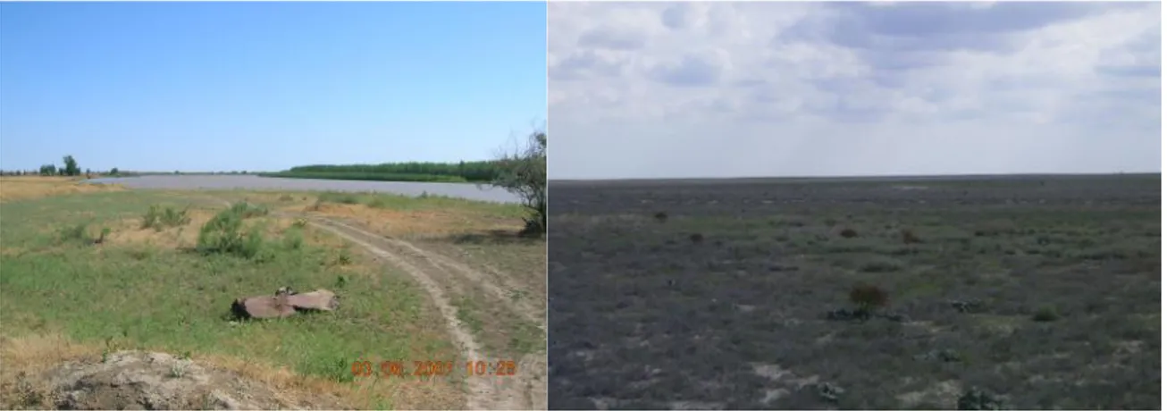
The DInSAR technique in wide uninhabited areas, even if already tested in environment similar to the Kazakh coast of the Caspian Sea, did not ensure high data coherence and a complete coverage of the area.The “experimental” application established that the terrain response to radar technique is suitable in this coastal zone, also in geomorphologically different areas (Frame Z3 has different characteristics if compared to Frames Z1 and Z2, as shown in Figure 1 and Figure 2).
Hence, the frames cover the all three "sides" of the coastland of the north-eastern Caspian and suffice to map the possible evolution of the present land subsidence acting in the study area.
Figure 1: Landscapes within Frame Z1, along the Ural river vegetated belt and Eskene area.
Figure 2: Landscapes within Frame Z3, Buzachi peninsula.
Looking within the available SAR archives, the most useful satellites to be used were ENVISAT-ASAR of the European Space Agency (ESA) and RADARSAT-1 of the Canadian Space Agency. Their acquisitions span the period from 2003-2004 to 2009. Unfortunately, ERS-1/2 satellites did not acquired over the north Caspian and therefore any analysis can be carried out during the 1990s. Since significantly more cheaper than RADARSAT-1 scenes, the ENVISAT-ASAR images have been used.
Figure 3: Study area subdivision
Applied methodologies are described in detail in following paragraphs. Models’ results have been compared with data recorded through DInSAR technique, considering especially
Zone A
Zone B
Zone C
uninhabited areas in which vertical displacements recorded are referred exclusively to natural sediments’ compaction. A brief discussion of the topic is given in 5.
The conceptual diagram below (Figure 4) shows the relevance of the geo-hydrogeological reconstruction during the development of this scientific research. It is a key step both for the interpretation of DInSAR interferometry results and for the implementation (choice - data input – results’ interpretation) of the models.
It has been outlined at different scales: Basin-scale:
At the basin-scale, three main geological provinces of the study area include: 1) Precaspian Basin
2) North Ustyurt Basin Local scale:
Four subareas of the northern part of the Caspian Sea have been identified.The subdivision has been identified according to the geologic asset of the area and the spatial distribution of InSAR interferometry analysis, which foresees the technical application in three 100x100 km frames (one for each onshore zone). The 4 selected zones include:
Zone (A) Transitional and offshore northern area;
Zone (B) Northern onshore area, from the Atyrau region to the Emba River valley; Zone (C) Eastern portion, from the Emba River valley to Mertviy Kultuk Bay;
Zone (D) Central portion of the Mangystau region, included in the North Ustyurt Basin.
Figure 4: Links between the geo-hydrogeological reconstruction and activities carried out during the analysis of present subsidence.
Main advantages and disadvantages, for every applied methodology, are listed below.
Table 1: Advantages and disadvantages of applied methodologies. Methodology of investigation Advantages Disadvantages Investigation of natural subsidence through 1D numerical model (NATSUB)
• High manageability of the code;
• Previous successfully applications in similar contexts (e.g., Northern Adriatic Sea);
• Since the model considers only one dimension, no lateral approximations are required; • Very accurate stratigraphical
information of the whole sedimentary column is available as input data;
• The model cannot consider dynamics related to salt diapirs;
• Assessment of compressibility calculated
from logs is not as reliable as laboratory tests, so the model’s results are “semi-quantitative”.
• As highlighted during Gap
Analysis, required information is localised in
Methodology of investigation
Advantages Disadvantages
• Availability of wireline logs, needed for compressibility calculation;
• Model’s application at 5 different locations, with 3 different compressibility trends;
• High local variability of shallow sediments’ geotechnical properties (up to 30 m) doesn’t cause strong variations in final results.
applications in onshore area of study are not allowed.
Investigation of natural subsidence
through 2D numerical model
(BASIN)
• The model provides a wide range of different results; • The model considers different
sedimentation rates from the southern border to the centre of the Precaspian basin.
• Heavy later approximations and simplifications are required during the implementation;
• Stratigraphic and chronostratigraphic
information required is not detailed outstanding the offshore area. Present vertical displacement investigation through DInSAR methodology
• It is the only way to perform analysis over past time interval (from 2003);
• Results confirm that it is ideal for subsidence assessment in wide and inaccessible onshore areas;
• Do not require field surveys; • Best rate between cost and
surface monitored;
• Its vertical movement resolution is about 2
• Vertical resolution (about 2 mm/y) is comparable to value of natural subsidence of the study area;
• Lack of permanent GPS stations that are required for the calibration of measurements;
• Adequate presence of point targets only within frame Z1; • Insufficient information about
Methodology of investigation Advantages Disadvantages mm/year; • Planar resolution is 40X40 meters;
• Its area of analysis (frame) is up to 100X100 km;
• Some areas present natural point targets.
dynamic;
• Insufficient information about ongoing human activities in the study area that can cause the lowering (or the uplift) of the terrain recorded by DInSAR application.
Obtained results allow to foresee possible vertical movements in the next future (trends projected till 2013) and to plan possible monitoring activities, with techniques already applied during this phase of study (e.g. acquisition of new SAR images) coupled with new ones (best potential solution for installation of fix GPS and best potential improvement of IPTA application through the installation of artificial Point Target).
The versatility of some of the techniques applied in this work allows us to hypothesize other activities that could be applied in the area of study in the future, as the study and monitoring of wider areas (at the moment not covered by the analysis), the use of other satellites in order to improve the SAR results in areas of particular interest, the creation of a Digital Elevation Model (DEM) from SAR images and an experimental application of InSAR analysis on the production islands to investigate possible differential displacements, potentially caused by the weight of the island and the expected anthopogenic land subsidence due to oil production.
3. GEO-HYDROGEOLOGICAL
RECONSTRUCTION
3.1 G
EOLOGY,
T
ECTONICA
NDS
EISMICITY3.1.1 Brief description of main geological features in the Caspian area
3.1.1.1 North and Middle area
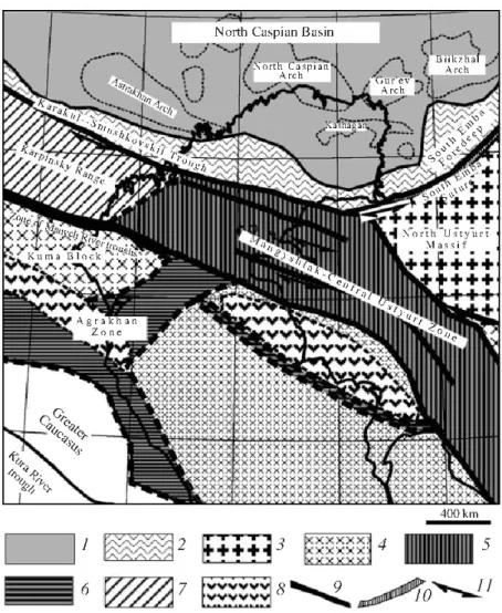
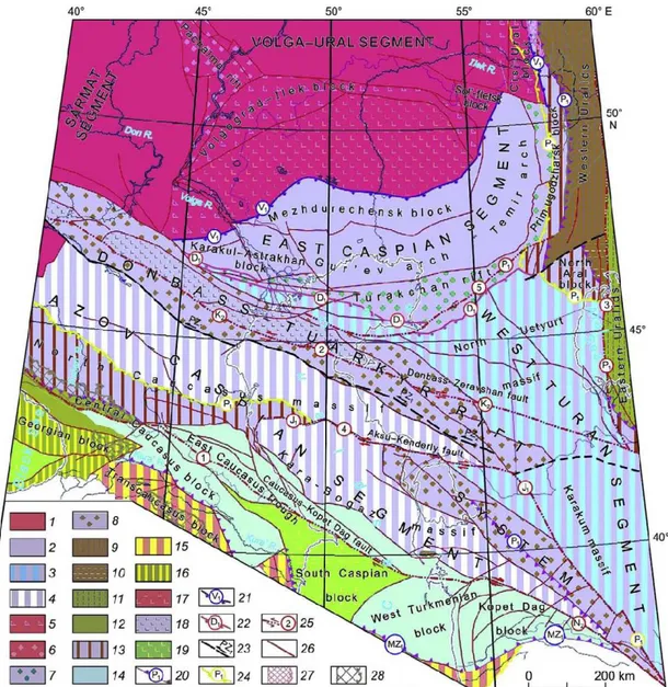
According to Afanasenkov et. al. (2008), the following structures are identified within the study region (Figure 5):
1. North Caspian Basin with a Central Depression and a Southern System of relative elevations of the Astrakhan–Aktyubinsk Zone;
2. Karakul–Smushkovskii Foredeep; 3. South Emba Foredeep;
4. Karpinsky Range Fold Zone;
5. Mangyshlak–Central Ustyurt Fold Zone; 6. South Emba Suture;
7. North Ustyurt Massif;
8. Prikumsk (Kuma) Block of Cis-Caucasus; 9. Agrakhan Zone;
10. Central Caspian Massif;
11. Alpine Orogen of the Greater Caucasus.
THE NORTH CASPIAN BASIN
The North Caspian Basin is filled with several sedimentary successions that was extensively examined from seismic data. The lower region fills a rift basin with strongly thinned continental or oceanic crust, and can be interpreted as a sinrifting basin. This succession has not been penetrated by bore holes and its age is, therefore, disputable: (1) Ordovician and (2) Middle Devonian. The former option is based on discoveries of Ordovician faunal complexes at the northern margin of the North Caspian Basin, where sediments that need to be studied fill graben-like troughs of Ordovician age at the opening of the Paleo-Ural Ocean, which could have a branch-like extension into the North Caspian Region. The second option is based on the wide distribution of Devonian rifting in the East European Platform with the presence of
Devonian normal faults on the western slope of the North Caspian Basin e.g., within the Don– Medveditsa Basin. A deepwater basin similar to that of the Red Sea could have originated during accumulation of the lower succession.
The second succession consists of sediments overlying the rifting complex (a post-rifting succession). The age of its base is debatable (either Silurian or Middle Devonian). Its upper boundary is conventional, traced to the beginning of the formation of a foreland basin at the Ural and Karpinsky Range orogens. A deepwater basin existed in the middle of this basin, bordered by passive continental margins and shelf basins. Conditions for originating carbonate edifices were favourable at the margins of the shelves.
The third succession was an orogenic complex filling the deepwater basin with clastic material from erosion of mountain ranges in the Uralian and Scythian orogens. The lower limit of the complex was Middle or Upper Carboniferous and the upper boundary was Triassic. The rise of the Ural Orogen commenced in the Middle Carboniferous, becoming the principal event by the beginning of the Permian. Under these conditions, supply of great amounts of clastic material began into the previously formed deepwater basins from the orogens associated with the Caspian Basin. The residual basin was filled with clastic material due to this avalanche-like sedimentation. A thick evaporite succession accumulated in the basin due to its nearly complete isolation from the World Ocean during the Kungurian Age.
The fourth succession is the Triassic post-rifting complex, which accumulated owing to thermal subsidence of the zone of the Paleozoic rift. The fifth succession is the Jurassic–Cenozoic platform cover overlying a considerable portion of the East-European Platform. The Astrakhan–Aktyubinsk uplift zone crowned with numerous Late Paleozoic carbonate edifices is traceable along the southern margin of the basin. According to gravity and magnetic data, the carbonate edifices may be underlain by Lower Paleozoic or Early – Middle Triassic volcanics (Segalovich et al., 2007).
Figure 5: Tectonic scheme of the North Caspian Region, after “A. P. Afanasenkov et. al., 2008”
1, North Caspian Basin; 2, Late Paleozoic Foredeep; 3, Precambrian terrane; 4, Paleozoic and Precambrian terranes; 5, Paleozoic zones with Triassic rift and pre-Jurassic inversion; 6, Paleozoic zones with Triassic
sediments of various facies and pre-Jurassic inversion; 7, , Karpinsky Range Zone of Early Permian Orogeny and Jurassic inversion; 8, Triassic volcanic belts; 9, zone of Manych River troughs with pre-Jurassic inversion; 10, South Emba Late Paleozoic Suture with pre-pre-Jurassic transpression; 11, strike-slip
faults of unclear kinematics.
KARAKUL–SMUSHKOVSKII FOREDEEP
The Karakul-Smushkovskii Foredeep is traceable along the northern margin of the Karpinsky Range. This zone was a shelf margin during the Late Devonian and Early–Middle Carboniferous, where carbonate edifices originated. Beginning in the Moscovian Age, the basin was filled with clastic material supplied from the Karpinsky Range and Scythian Orogen, that is, the shelf basin began transforming into a foredeep. The maximum fill-up of the basin with clastic material of a flysch–molasse succession was during the Asselian Age. The foredeep was transformed into a fold-nappe zone prior to the Kungurian Age (possibly during the Sakmarian Age).
SOUTH EMBA FOREDEEP (INCLUDING THE MYNSUALMAZ FOLD ZONE)
South Emba Foredeep is formally a continuation of the Karakul–Smushkovskii Zone. The principal difference between the two lies in the fact that the subsidence of this basin as a foredeep took place during the Devonian and Visean ages. Its clastic material included fragments of mafic and intermediate volcanics, jasper, limestone, serpentinite, and tuffs; this implies that these sediments originated due to erosion of the orogenic rock complex with fragments of ophiolites and island-arc rock associations. The South Emba is interpreted as a suture that collided with the North Caspian Basin and North Ustyurt terrain, subsequently transformed into a pre-Sinemurian strike-slip zone.
KARPINSKY RANGE FOLD ZONE
The Karpinsky Range Fold Zone mostly consists of Carboniferous schists and interlayered siltstones more than 10 km thick. This succession is strongly deformed, with overthrusts and duplexes playing an important role in its structure. The rock complex of the Karpinsky Range was thrust northward over the Karakul–Smushkovskii Zone in Early Permian (most likely during the Sakmarian Age). The Karpinsky Range lies on a continuation of the Devonian Rift in the Donets Basin, and there is the possibility that the basin within the Karpinsky Range was a rift trough (possibly, a backarc basin) during the Devonian. During the Early–Middle Triassic, rift basins formed within the Karpinsky Range region. These were strongly deformed, and inversion took place at approximately the Triassic–Jurassic boundary; therefore, Triassic basins within secondary (after deformations and erosion) contours can be traced. Since the Jurassic, the Karpinsky Range became a portion of the sedimentary basin of the East European Platform.
MANGYSHLAK–CENTRAL USTYURT FOLD ZONE
The Mangyshlak-Central Ustyurt Fold Zone shows a complex structure vaguely understood due to its overlain basement virtually everywhere by thick cover. The following tectono-stratigraphic units have been recognized within its folded complex: Lower Paleozoic; Devonian–Middle Carboniferous; Upper Carboniferous–Lower Permian; and Upper Permian– Triassic. The Lower Paleozoic unit is hypothetical and may represent metamorphic complexes. The Middle Devonian–Carboniferous succession encloses ophiolites and deep-water sediments (Tuarkyr Rise) definitely originated under conditions of an oceanic basin and its closing. The Upper Carboniferous–Lower Permian succession includes carbonates of different facies, clastic rocks, and subduction-related volcanics. All these rocks originated during the collision stage of the orogen evolution. A complex orogen formed in the Mangyshlak–Central Ustyurt Zone by the Middle Permian time (in the Early Permian), though its structure is not known in detail. The orogen extended southward from the South Emba Suture and completely embraced the southern part of the contemporary Turan Platform. The Hercynian orogen
collapsed during the Kungurian Age and the Late Permian Epoch (that is, a system of fault-bounded orogenic extension troughs formed in its place), and molasse-filled basins were widespread in this region.
Rifting was very common throughout the whole region during the Early Triassic, which was accompanied by formation of deep (up to 3–5 km) rifting basins. One such rift is currently under the Kulaly Swell. The Triassic rifts are located north of the Early–Middle Triassic volcanic belt and, hence, backarc extension is the most probable cause of the rifting.
Strong compression of the region took place at approximately the Triassic–Jurassic boundary. Most rift basins experienced inversion there accompanied by folding and overthrusting deformations. Strike-slip displacements of individual blocks considerably complicated the deformations. The presence of strike-slip faults is noted, but there is zero possibility of reconstructing the motion kinematics along the zone where displacements could reach hundreds of kilometres. Since the Jurassic, the Mangyshlak–Central Ustyurt Zone became a portion of a vast platform-type sedimentary basin.
NORTH USTYURT MASSIF
This massif with Precambrian metamorphic basement is viewed as a terrain of continental crust that collided in the Late Devonian–Visean with a margin of the North Caspian Basin, which was probably a part of the Late Paleozoic Turanian Orogen.
PRIKUMSK (KUMA)BLOCK
This block within the Cis-Caucasian region is a terrain in the Late Paleozoic Orogen with Mesozoic–Cenozoic sedimentary cover.
AGRAKHAN BLOCK
Afanasenkov, et. al. (2007) recognized the Agrakhan Block conditionally as a fragment of the Hercynian Orogen overlain both by sediments and volcanics. The block is poorly studied thus far.
CENTRAL CASPIAN MASSIF
This is a massif resultant from the Hercynian Ustyurt Orogen.
3.1.1.2 Southern area
The South Caspian is located over a high-velocity (Vp = 7 km/s) thin (10–18 km) basement has often interpreted as an oceanic basin filled with ∼20 km of sediments (e.g., Allen et al., 2002). However, the sedimentary thickness is about twice that needed to fill a basin upon oceanic crust as thick as that in the South Caspian. Maintaining consolidated crust at a depth of 20 km requires 20–25 km of eclogites, denser than mantle peridotites, to occur under the
Moho. According to its chemistry, eclogites belong to the crust but have typical mantle seismic velocities, and are thus placed beneath the Moho in many seismic models.
The Moho in the South Caspian basin is overlain by high-grade felsic and intermediate rocks with P velocities up to 7 km/s. Its high density is due to metamorphism with the formation of garnet at T ≥ 400 °C. With eclogites lying under the Moho, the basin basement totals a thickness of 40–50 km, which corresponds to a continental crust.
Crustal subsidence in the South Caspian was induced by a phase change of gabbro into denser eclogites. Subsidence occurred at rapidly increased rates at least twice, at the Eocene/Oligocene boundary and during the Pliocene-Pleistocene time.
The first episode of rapid subsidence produced (or deepened) a marine basin and a subsequent episode was associated with a deposition of a 10 km thick sedimentary succession in 5 Myr. The increased subsidence rates may have been due to the effect of active fluids that catalyzed the gabbro-eclogite transition. Rapid subsidence as occurs in the South Caspian is impossible upon oceanic crust. Rapid and major crustal subsidence was found typical of hydrocarbon basins (Artyushkov and Yegorkin, 2005). The reliability of this criterion as a diagnostic for the discovery of hydrocarbon reservoirs elsewhere was confirmed by the evidence of rapid subsidence in the large petroleum province of South Caspian.
The rapid Pliocene-Pleistocene subsidence in the South Caspian with a deposition of 10 km-thick sediments was explained in terms of a flexural basin developing in front of a subduction zone in the south or in the north (Allen et al., 2002; Axen et al., 2001; Knapp et al., 2004). However, even though it existed, the flexure could be located within a wide zone of a few kilometres along the Apsheron-Balkhan sill that caused no influence on subsidence outside that strip. Judging by the presence of steep basement flexures up to 10–12 km deep,the lithosphere of the South Caspian apparently experienced strong softening as a result of fluid infiltration during the recent rapid subsidence.
Relatively large historic earthquakes (M = 5–6) located at depths of ≥ 30 km beneath the Apsheron-Balkhan sill and north within a ∼ 100 km wide zone were interpreted as an indication of northward subduction. The consolidated lithosphere as in the South Caspian basin, with its density higher than the asthenosphere due to phase change, could in principle be involved in subduction with delamination of the overlying lighter sediments on condition of strong lateral compression and softening. Had subduction occurred in the South Caspian, the subduction plate would have been ∼ 100 km long, and the delaminated sediments would have experienced shortening of the same magnitude. Yet, judging by very shallow fold dips in the area, shortening was no more than 5–10 km. Therefore, hardly any subduction occurred.
Furthermore, slopes of oceanic trenches on active margins are normally dominated by compression but most earthquakes in the northern South Caspian show extension mechanisms. The earthquakes originate mostly in the crust (at 30 to 50 km) and show no alignment like a Benioff zone. Therefore, the basin with its thick sedimentary fill lies over continental crust, and the extension focal mechanisms may record normal faulting associated with ongoing consolidation of mafic rocks by eclogitization (Artyushkov, 2007).
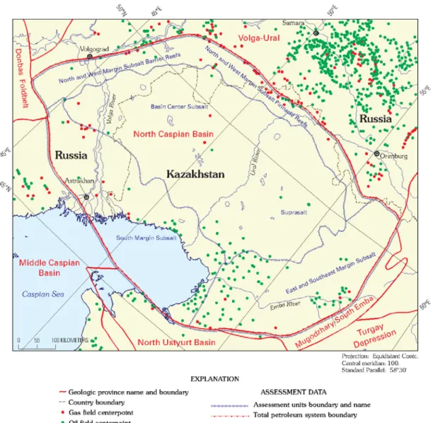
3.1.2 The North Caspian Basin Structure
The North Caspian Basin province occupies the northern part of the Caspian Sea and a large plain to the north (Figure 6) and covers some 500,000 km2.
Figure 6: Petroleum system and assessment units of North Caspian Basin. After G. F. Ulmishek, 2003”.