PAPER • OPEN ACCESS
Two-membrane cavity optomechanics
To cite this article: Paolo Piergentili et al 2018 New J. Phys. 20 083024
View the article online for updates and enhancements.
PAPER
Two-membrane cavity optomechanics
Paolo Piergentili1,2 , Letizia Catalini1, Mateusz Bawaj1,2 , Stefano Zippilli1,2 , Nicola Malossi1,2 ,
Riccardo Natali1,2 , David Vitali1,2,3,4 and Giovanni Di Giuseppe1,2,4
1 School of Science and Technology, Physics Division, University of Camerino, I-62032 Camerino(MC), Italy 2 INFN, Sezione di Perugia, Italy
3 CNR-INO, L.go Enrico Fermi 6, I-50125 Firenze, Italy 4 Author to whom any correspondence should be addressed.
E-mail:[email protected]@unicam.it
Keywords: optical cavity, optomechanical systems, radiation pressure
Abstract
We study the optomechanical behaviour of a driven Fabry–Pérot cavity containing two vibrating
dielectric membranes. We characterize the cavity mode frequency shift as a function of the
two-membrane positions, and report a
∼2.47 gain in the optomechanical coupling strength of the
membrane relative motion with respect to the single membrane case. This is achieved when the two
membranes are properly positioned to form an inner cavity which is resonant with the driving
field.
We also show that this two-membrane system has the capability to tune the single-photon
optomechanical coupling on demand, and represents a promising platform for implementing cavity
optomechanics with distinct oscillators. Such a configuration has the potential to enable cavity
optomechanics in the strong single-photon coupling regime, and to study synchronization in optically
linked mechanical resonators.
1. Introduction
Multi-element systems of micro/nano-mechanical resonators offer promising prospects for enhanced optomechanical performances[1–7], coherent control [8,9], and for the exploration of multi-oscillators
synchronization[8,10–16]. The standard path for reaching the strong single-photon optomechanical coupling
regime is to consider co-localized optical and vibrational modes[17–19], with a large spatial overlap confined in
very small volumes, corresponding to mechanical modes with extremely small effective mass. An alternative solution, capable of providing systems with orders of magnitude increased ratio between the single-photon optomechanical coupling rate, and the cavity decay rate, is to exploit quantum interference in multi-element optomechanical setups[3–5]. Although the simplest two-membrane sandwich in an optical cavity is a paradigm
for the realization of strong-coupling optomechanics, and the observation of collective mechanical effects(such as synchronization), no experimental studies of these phenomena have been reported till now. Previous related results[20] were confined only to the optical and mechanical characterization of two-membrane sandwiches.
Here we report on thefirst experimental characterization of the optical, mechanical, and especially optomechanical properties of a sandwich constituted of two parallel membranes within an optical cavity. We show how the resonance frequencies of the optical cavity are shifted as a function of the position of the two membranes. This effect is central to the description of the optomechanical properties of the system, since it provides a direct estimation of the strength of the couplings[1,21–23]. By investigating the shifts of the cavity
resonances wefind that the optomechanical coupling strength is enhanced by constructive interference when the two membranes are positioned to form an inner cavity which is resonant with the drivingfield. Specifically we determine a gain of∼2.47 in the coupling strength of the relative mechanical motion with respect to the single membrane configuration. We finally prove both the capability to tune on demand the single-photon optomechanical couplings, and the simultaneous optical cooling of the fundamental modes of the two distinct membranes. OPEN ACCESS RECEIVED 24 May 2018 REVISED 27 July 2018
ACCEPTED FOR PUBLICATION
6 August 2018
PUBLISHED
17 August 2018
Original content from this work may be used under the terms of theCreative Commons Attribution 3.0 licence.
Any further distribution of this work must maintain attribution to the author(s) and the title of the work, journal citation and DOI.
2. Theory
Generalizing the results obtained in[5], we consider the case of two different movable dielectric membranes
placed inside a Fabry–Pérot cavity of length L, which is driven by an external laser. The Fabry–Pérot cavity is composed of two identical mirrors with electricfield reflection and transmission coefficients r and t, respectively. The membranes can be modelled as dielectric slabs of thickness Lm,jand index of refraction nj (where the index j=1, 2 distinguish the parameters of the two membranes), such that their reflection and transmission coefficient can be expressed as
= -+ + ( ) ( ) ( ) ( ) ( ) ( ) r n kn L n kn L n kn L 1 sin 1 sin 2i cos , 1 j j j j j j j j j j 2 m, 2 m, m, = + + ( ) ( ) ( ) ( ) t n n kn L n kn L 2 1 sin 2i cos , 2 j j j2 j m,j j j m,j
where k=2π/λ is the wavenumber of the electric field, and λ is its wavelength.
The optical resonance frequencies correspond to the maxima of transmission of the whole cavity. The electricfield amplitudes Ajof incident( j=in), reflected ( j=ref), and transmitted ( j=tran) waves, as well as for thefields in the cavity ( j=1, 2, K, 6) (see figure1), satisfy the following equations:
= - ( ) A it A r A e kL, 3 1 in 2 i 1 = - ( ) A it A e kL r Ae kL, 4 2 1 4 i 2 1 1 i 1 = - ( ) A it Ae kL r A e kL, 5 3 1 1 i 1 1 4 i 2 = - ( ) A it A e kL r Ae kL, 6 4 2 6 i 3 2 3 i 2 = - ( ) A it A e kL r A e kL, 7 5 2 3 i 2 2 6 i 3 = - ( ) A r A e kL, 8 6 5 i 3 = - ( ) A it Ae kL r A , 9 ref 2 i 1 in = ( ) A it Ae kL, 10 tran 5 i 3
where Lj=qj−qj−1(with qjthe positions of the various elements defined in figure1, and j=1, 2, 3) is the length of the subcavities formed by the mirrors and the membranes, so that L=L1+L2+L3. We point the reader to[22] for a similar approach in the case of a single membrane. Here we use the same convention of [22]
for the scattering matrix of a single scattering element, either the cavity mirror or the membrane. This is a bit different from the choice of[5], which is reproduced by replacing r with −r into the equations above.
Equations(1)–(10) are valid, for any value of the thickness, in the ideal one-dimensional case of plane waves, and
flat, aligned mirrors and membranes. They can be applied also to the case of Gaussian cavity modes and spherical external mirrors as long as the membranes are placed within the Rayleigh range of the cavity.
The system of equations(3)–(10) can be solved to determine the transmission coefficient of the whole cavity.
It is given by t = = ( ) A A t t t e , 11 c kL tran in 2 1 2 i
Figure 1. Schematic diagram of the system. Two movable dielectric membranes are placed inside a Fabry–Pérot cavity of length L which is driven by an external laser. The position of twofixed mirrors (movable membranes) is denoted by q0and q3(q1and q2); we
with = - + + + + + + + - - -+ + + ( )( ) ( ) ( ) ( ) ( ) ( ) ( ) r t r t r rr t r r r r rr t r rr r r rr 1 e e e e e e e . 12 kL k L L k L L k L L kL kL kL 2 12 12 22 22 2i 2 12 12 2i 2 1 2 2i 1 22 22 2i 1 2i 1 2 2i 2 2i 1 2 1 3 2 3 1 2 3
This last expression reproduces equation(4) of [5] when r1=r2, t1=t2, and we restrict to the case of real nj, implying in particulararg( )rj =arg( )tj ºfjso thatrj2+tj2=e2ifj. Moreover it reproduces also the case of a
single membrane which is obtained by takingr2=0,t2= -i,L3=0. From equations(3)–(10) one can also derive the expression for the reflectivity, given by
= = - + - -- + -+ [ ( ) ] ( ) ( ) ( ) A A r t r rr t t r r r t rr e 1 e e e 1 e . 13 c kL kL k L L kL kL refl in 2 1 2i 1 2i 2 12 2i 2 22 22 2i 1 2i 1 1 1 2 3 1
An explicit equation for the cavity mode frequencies can be found in the case of negligible optical absorption of the membranes, i.e. for real nj. In this case we rewrite rjwith j=1, 2 in terms of the intensity reflectivity Rjas
= f
rj R ej ij, and we assume for simplicity r and t real so that we express them in terms of the corresponding
intensity reflectivitys as = -r R t, = - 1-R. Accordingly, equation(12) becomes
= - -+ -+ -+ f f f f f f f f f f f f + + + + + + + + + + + + + + + ( ) ( ) ( ) ( ) R RR R R R RR RR R R RR 1 e e e e e e e . 14 kL k L L k L L k L L kL kL kL 2i 2i 2i 2 2i 2i i 1 2 2i i i 1 2i i 2i 1 2i i 1 2 2i i i 2 2i i 1 2 1 2 1 2 1 3 1 2 2 3 1 2 1 1 2 1 2 3 2
The cavity mode frequencies correspond in general to the maxima of the transmission, and therefore the minima of∣ ∣2. In the limiting case of perfect external mirrors, R=1, these maxima become poles of the transmission and the modes correspond to the zeros of . In order to get a simple expression for the poles we restrict to this limiting situation which, as we have seen in[5], works also in the case of realistic high-finesse cavities for which
typically 1−R∼10−5. In particular using the definitionsL1=q1+L 2,L3=L 2-q2and introducing the relative coordinateq=L2=q2-q1wefind that equation (14) can be rewritten, for R=1, as
f f f f - = + + - -- - + + ( ) ( ) ( ) ( ) ( ) kL R R kL kq R kq R kq 2i sin sin 2 sin 2 sin 2 . 15 1 2 1 2 1 1 2 2 2 1
By setting this equation equal to zero we get the implicit equation for the cavity mode frequencies valid in the limit of R∼1 and for the general case of two different membranes. It reproduces the implicit equation in the two special cases of equal membranes and of one membrane only. Specifically, in the case of equal membranes R1=R2=Rm, f1=f2=f, and using the definitionsL¢ ºL+2f kandq¢ º +q f k q, 1=Q-q 2,q2=Q+q 2, where Q=(q1+q2)/2 is the center-of-mass (CoM) coordinate, we get
¢ - ¢ - ¢ + ¢ =
(kL) R (kL kq) R ( kQ) (kq) ( )
sin msin 2 2 mcos 2 sin 0, 16
which coincides with equation(8) of [5]. Instead in the one membrane case, puttingR2=0,f1=fand f2=−π/2, we get
f
-cos(kL+ )- R1cos 2( kq)=0, which is just the corresponding equation used in[24] in the limit R=1.
In the general case the implicit equations for the mode frequencies = 0, with given in equation(15), can
be expressed using the definitionsL¢ º L+f1 k+f2 k q, ¢ º +q f1 2k+f2 2k, andQ¢ º Q+ Df 4 ,k (Δf=f1−f2), as
(kq¢)sin(kL¢ +) (kq¢)cos(kL¢ =) (kQ kq¢, ¢), (17) with (kq¢ = -) 1 R R1 2cos 2( kq¢),(kq¢ =) R R1 2sin 2( kq¢), and (kQ kq¢, ¢ =) R1sin 2( kQ¢ -kq¢ -)
¢ + ¢
( )
R2sin 2kQ kq . This can be further simplified with the definitionsO˜ =O 2+2,O= , , such that equation(17) can be rewritten in the equivalent form
q ¢ + ¢ = ¢ ¢ [kL (kq)] ˜ (kQ kq) ( ) sin , , 18 where ¢ ¢ = ¢- ¢ - ¢+ ¢ + - ¢ ˜ ( ) ( ) ( ) ( ) ( ) kQ kq R kQ kq R kQ kq R R R R kq , sin 2 sin 2 1 2 cos 2 , 19 1 2 1 2 1 2
and q ¢ = ¢ = ¢ + - ¢ ⎪ ⎪ ⎪ ⎪ ⎧ ⎨ ⎩ ⎫ ⎬ ⎭ ( ) [ ˜ ( )] ( ) ( ) ( ) kq kq R R kq R R R R kq
arcsin arcsin sin 2
1 2 cos 2
, 20
1 2
1 2 1 2
and which, in turn, is equivalent to its formal solution obtained by inverting the sin function, that, using the definition ofL¢, can be expressed as
p p =ℓ + ( ¢ ¢) ( ) k L kQ kq, 21 with p (kQ kq¢, ¢ = -) ( 1 arcsin)ℓ [ ˜ (kQ kq¢, ¢ -)] q(kq¢ -) f -f (22) 1 2
andℓinteger. For each value of ℓone finds a solution for a cavity mode wavenumber kℓthat can be decomposed as the sum,kℓ=kℓ( )0 +dkℓ, of the empty cavity solution ℓ = ℓp
( )
k0 L(which corresponds to the condition R1=R2=0, that implies ˜ (kQ kq¢, ¢ =) q(kq¢ =) 0) and the shift due to the membranes that is given by the implicit expressiond = -p( ¢ ¢) ℓ ℓ ℓ k L 1 k Q k q, . In typical experiments, l= p ℓ ( ) k L
2 0 , so thatℓis a very large integer and this implieskℓ( )0 dkℓ. In this limit one can safely take ¢ +f ℓ +f ℓ
( ) ( )
L L 1 k0 2 k 0 and
f f
¢ + ℓ( )+ ℓ( )
q q 1 2k0 2 2k 0. Correspondingly, for R1and R2not too close to one, and for not too large values of q1and q2, i.e., when q1/L, q2/L=1, (see [5]), one can safely express the shift explicitly as a function of the empty cavity solution asd = -p( ¢ ¢)
ℓ ℓ ℓ
( ) ( )
k L 1 k 0Q k, 0q , that can be also written as an equation for the cavity mode frequency shift[5] dw d p p l pl º = ⎜⎛ ⎟ ⎝ ⎞⎠ ( ) ( ) c k c L q q 2 , 2 . 23 m0 1 2
This treatment in the general case of two different membranes generalizes previous results and has the advantage of providing a unique framework in which one can immediately compare the single and two-membrane case. On the other hand, for a given value of the maximum available membrane reflectivity Rmax=max{R1, R2}, we have numerically verified that the largest optomechanical couplings are achieved when the two membranes have identical reflectivities. For this reason we have focused our experiments to the case of nominally identical membranes, and we shall restrict from now on to this latter case. In particular, introducing the parameters =m R1=R2, and f=f1=f2,Lm=Lm,1=Lm,2and n=n1=n2, the explicit dependence upon the variables kq1and kq2of the parameters ˜ (kq kq1, 2)and q (kq kq1, 2)that enter into the definition ofin equation(22), is easily obtained from equations (19) and (20), so that for identical membranes one has
f f = - + - + + - - + ˜ ( ) [ ( )] [ ( ) ] [ ( ) ] ( ) kq kq k q q k q q k q q , 2 cos sin 1 2 cos 2 2 , 24 1 2 m 1 2 2 1 m 2 m 2 1 q f f = - + + - - + ⎡ ⎣ ⎢ ⎢ ⎤ ⎦ ⎥ ⎥ ( ) [ ( ) ] [ ( ) ] ( ) kq kq k q q k q q , arcsin sin 2 2 1 2 cos 2 2 . 25 1 2 m 2 1 m 2 m 2 1
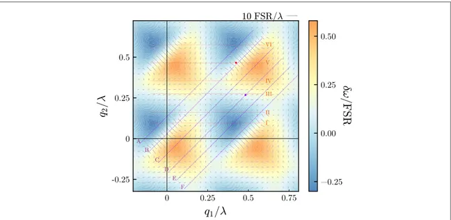
Figure2shows the mode frequency shiftδω normalized to the free-spectral-range of the cavity, FSR=π c/L, as a function of the membrane positions q1and q2normalized to the wavelength, assuming the parameters of the experimental setup, i.e.,l = 1064 nm,=0.999 94,L=90 mm,Lm=104 nm, and n=2.17. It is worth noting that a nonzero value of the phasef determines a displacement of the pattern along the bisector of the second and fourth quadrants, and a constant shift of the cavity frequencies.
The optomechanical couplings strength Gjare the derivative of the optical mode frequencies with respect to the position of the jth membrane qj. Defining the scaled dimensionless positionsq˜j=qj l, we can write in general l p p = ¶ ¶ ( ˜ ˜ ) ˜ ( ) G q q q FSR 2 , 2 . 26 j j 1 2
In the case of a single membrane the single-photon optomechanical coupling has the same structure of equation(26) l p = ¶ ¶ ( ˜) ˜ ( ) G q q FSR 2 , 27 sing sing
but with a different dimensionless frequency shift function
p (2pq˜)= -( 1 arcsin)m [ cos 4( pq˜)]. (28)
sing m
Taking the derivative one can see that the maximum value of ¶ sing(2pq˜) ¶q˜is4 m(halfway between a node and an antinode of thefield), so that
l
= ( )
Gsingmax FSR 4 m. 29
In order to study the enhancement of the coupling(and the associated optical interference effect) due to the presence of the second membrane, we have to compare the maximum derivative of the function p(2 q˜1, 2pq˜ )2 with respect to4 m. Infigure2we show the cavity mode frequency shifts, and superimposed the vector plot of the corresponding gradientfield, which gives the values of the two couplings G1and G2. It shows that the largest optomechanical coupling is achieved simultaneously by the two membranes, and in this case G1=−G2. At this point the cavity mode frequency is sensitive atfirst order only to the variation of the distance between the two membranes, q=q2−q1, and is not sensitive to shifts of the CoM of the two membranes, Q. This implies that the coupling of the CoM is zero, GQ=0, while that of the relative coordinate is∣Gq∣=∣ ∣Gj[5]. In this case,
in order to determine the gain factor we apply the same argument of section III of[5] from equations (19)–(23).
Specifically, we find that, for ℓ integer p = + - + -∣ ∣ ( ) [ ( ˜ ˜ )] ∣ ∣ ( ) ℓ G 1 cos 2 q q G 1 . 30 jmax m 1 2 m singmax
This means that the maximum coupling for both membranes is achieved when( ˜q1+q˜ )2 is an integer number for evenℓ, and an half-integer for odd ℓ (and this is visible also from the vector plots in figure2). Using this
condition equation(30) reduces to
= -∣G ∣ 1 ∣G ∣ ( ) 1 . 31 jmax m singmax
In the case of = 0.4m , as in our experiment, the optomechanical coupling may increase up to a factor∼2.72. As discussed in detail in[5] (see also [3,4]), the present treatment based on the assumptionkℓ( )0 dkℓ,
allowing to express the frequency shift explicitly as a function of the empty cavity solution(see equation (23)), is
valid provided that the reflectivity mis not too close to one. This fact could be guessed from the fact that equations(30)–(31) suggest an unlimited value of the optomechanical coupling when 1m , which is unphysical. In fact, as numerically shown in[5] and could be expected also on physical grounds, when
m R~1(that is, the membrane reflectivity becomes equal or larger than the cavity mirror reflectivity), equation(30) is no more valid, and the optomechanical coupling saturates to a value corresponding to that of the
inner Fabry–Perot membrane cavity with lengthq G,∣ jsat∣=ckℓ( )0 q = 2pc (lq). As underlined in[5], when
∣q L∣ 1 and ~m R~1, this saturation value would still correspond to the strong-coupling regime where the single-photon optomechanical coupling is equal or larger than the cavity decay rate, because for aligned membranes with negligible absorption, the cavity decay rate remains identical to the value of the main cavity
Figure 2. Contour plot of the frequency shift functiondw=c kd ( )
m0for even m normalized to the free-spectral-range of the cavity, p
= c L
FSR , as a function of the membrane positions q1and q2normalized to the wavelength, due to the presence of the
two-membrane cavity. The parameters used for the numerical analysis are:l =1064 nm,=0.999 94,L=90 mm,Lm=104 nm, and n= 2.17. Superimposed the vector plot of the gradient field of the frequency shift, whose components give the two
optomechanical couplings, with the unit indicated on the top-right of the panel. The oblique blue lines(A–F) indicate the
experimental spectra obtained by varying the CoM of the membrane-cavity system for different positions q2, and reported infigure8.
The horizontal red lines(I–VI) indicate the experimental spectra obtained by varying q1for different positions q2, and reported in
with length L. In our experiment with commercially available membranes we are far from the condition m R~1, and therefore equations(30)–(31) can be safely used to describe the results.
3. Membrane-sandwich characterization
In our experiment we used two different membrane sandwiches. Thefirst is constituted of two low-stress SiN square membranes, with a side of1 mm, and a thickness of 100 nm. And the second is made of two high-stress Si N3 4square membranes, with a side of 1.5 mm, and a nominal thickness of 100 nm. In both cases, one of the membranes is glued on a piezo, which allows for a scan of the membrane-cavity length, while the whole
membrane-cavity mount is attached to another piezo in order to displace in a controlled way the CoM of the two membranes.
3.1. Optical properties
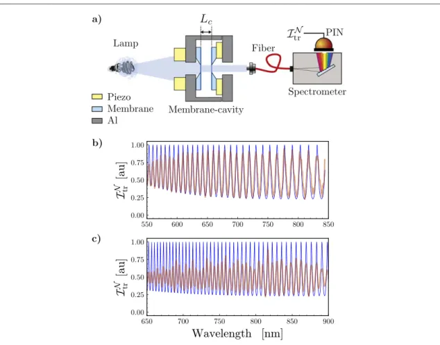
Here we report on the characterization of the two-membrane sandwiches in terms of reflectivity mand cavity length Lc, which we have performed before inserting them into the optical cavity. In particular, the membrane-cavity length Lcwas determined by illuminating the membrane-sandwich with a tungsten lamp. The transmitted light was collected by a multi-modefiber, and finally revealed by a spectrometer. The interference pattern of the normalised transmitted light is shown infigures3(b) and (c), for the first and second sandwich, respectively, and
compared with a best-fit curve obtained from the expression of the transmitted light
p = +[ (D ) ] ( ) 1 2 sin 2 , 32 tr in 2
where inis the input light intensity,Δ=4π Lc/λ, andis thefinesse of the membrane-cavity. From the spectrometer data of thefirst sandwich, figure3(b), we obtain a best-fit value for the membrane-cavity length
m
=
Lc 24.008 0.004 m. Moreover, assuming afinesse given by the equation
Figure 3. Cavity-frequency scan.(a) Experimental setup for cavity frequency-scan. The light of a tungsten lamp transmitted by the membrane sandwich of length Lcat rest, is coupled to a multi-mode opticalfiber and collected into a spectrometer for wavelength
analysis.(b) Red line represents the measured light transmitted by the first membrane-cavity, and normalised to the light in the absence of membranes, tr. Blue line is the best-fit obtained withLc=24.008 0.004 mm , andLm=100.0 0.2 nm.(c) Red
and blue line represent data from the second sandwich and best-fit, respectively. The best-fit providesLc=53.571 0.009 mm , andLm=106 1 nm.
p = -⎡ ⎣ ⎢ ⎢ ⎛ ⎝ ⎜ ⎞ ⎠ ⎟⎤ ⎦ ⎥ ⎥ ( ) 2 arcsin 1 2 , 33 m m 1
which holds in the case of equal membrane reflectivity, and using the values of the index of refraction provided by the manufacturer, wefind that the corresponding membrane thickness isLm=100.00.2 nm. From the data of the second sandwich,figure3(c), we obtain a membrane-cavity lengthLc=53.5710.009 mm , and a membrane thicknessLm=1061 nm, which is found for the index of refraction of Si3N4given in[25].
Although the membrane-cavity length is well estimated by the peak distances in the interference patterns reported infigures3(b) and (c), the membrane thickness, and consequently the reflectivity of the membrane, is badly derived by
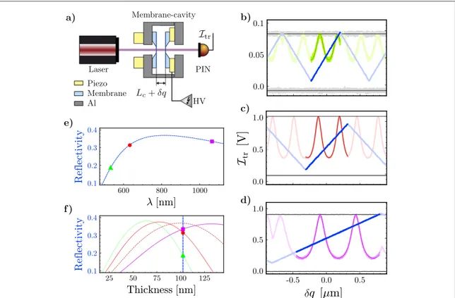
the poor visibility of the curves, measured with an apparatus not optimized for this purpose. The membrane reflectivity mat specific wavelengths is optimally estimated with a different experiment(see figure4(a)) exploiting again equation(32) and (33), but now collecting on a photodiode the light of a laser transmitted through the
membrane-cavity while scanning the membrane-cavity length q=Lc+δq, such that, in thiscase, we use Δ=4π q/λ in equation (32). For thefirst sandwich we use a1064 nm laser, and the best-fit provides a value of the finesse =3.26 0.02, yielding a corresponding value for the reflectivity =m 0.408 0.002. Such a result is consistent with a membrane thickness ofLm=104 1 nm, assuming an index of refraction n=2.17. Those values are in accordance with the ones provided by the manufacturer. For the second sandwich we used three different wavelengths, 532 nm, 632.8 nm and 1064 nm, and the corresponding results, obtained while scanning the cavity length, are shown infigures4(b)–(d). The
best-fit of equation (33) provides a value of the finesse and of the corresponding reflectivity for each wavelength. They
are given by 532=1.466 0.002,632.8=2.3817 0.0007, and 1064=3.20 0.03with corresponding reflectivity 532m =0.2050 0.0002,632.8m =0.3137 0.0001, and 1064m =0.3345 0.0003,
respectively. In order to estimate the thickness of the membranes these values werefitted according to the relation in equation(1) (see figure4(e)). As shown in figure4(f), we obtain a membrane thickness ofLm=102.3 0.1 nm.
Figure 4. Cavity-time scan.(a) Experimental setup for cavity time-scan. A PIN photodiode detects the light transmitted by the membrane-cavity while the membrane distance is scanned by means of a high voltage(HV) applied to a piezo. Light transmitted by the membrane-cavity for three different wavelengths,532 nm(b), 632.8 nm (c), and1064 nm(d), as a function of the membrane
distanceLc+dq. The best-fit values of the membrane-cavity finesse are 532=1.466 0.002,632.8=2.381 7 0.0007, and
1064=3.200.03), which correspond to membrane reflectivities 532m =0.2050 0.0002,m632.8=0.3137 0.0001, and
1064m =0.33450.0003, respectively. Blue line represents the voltage applied to the piezo.(e) Variation of the reflectivity of the membranes as a function of the wavelength. Green triangle, red circle and purple square are the measured reflectivity values at
532 nm, 632.8 nm, and1064 nm, respectively. The best-fit, blue curve, associated to equation (1), provides a value of the membrane
thickness ofLm=102.3 0.1 nm.(f) Dependence of the reflectivity of aSi N3 4membrane on the thickness(equation (1)), for three
different wavelengths:532 nm, 632.8 nm, and1064 nm. Dashed blue line represents the estimated thickness of the measured substrates[Lm=102.3 0.1 nm].
This result is estimated by using the values of the refractive index at the three wavelengths reported in[25], which are in
accordance with the ones provided by the manufacturer. 3.2. Mechanical properties
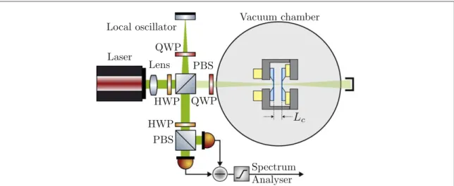
Here we present a study of the mechanical properties of the second membrane-sandwich by using a 532 nm laser in a Michelson interferometer, as shown infigure5[26] (this kind of study is not possible with the first sandwich due to the
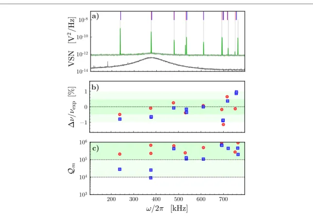
poor quality of the mechanical modes). In figure6we show the thermal voltage noise(VSN) of the two-membranes cavity revealed by homodyne detection of the reflected light, the quality factormof the mechanical modes, and the
relative difference between experimental andfitted mechanical frequencies. The membranes are very similar and show a set of very close resonance peaks. As shown infigure6(b), we reproduced the mechanical resonance frequencies of
both membranes with an error smaller than 1% assuming rectangular membranes and the nominal values provided by the manufacturer for the stress, s = 0.825 GPa, and for the density r =3100 kg m-3, and taking the side lengths asfitting parameters. Best-fit values areLx( )1 =1.519 0.006 mm, Ly( )1 =1.536 0.006 mm, and
= =
( ) ( )
Lx2 1.522 0.006 mm, Ly2 1.525 0.006 mm. Figure6(c) shows that the mechanical quality factor
changes significantly between the modes and that one membrane tends to have lowermvalues. We attribute these
scattered values to the effect of clamping which strongly depends upon the shape of the vibrational mode and may be different on the two membranes with the current mounting.
4. Estimation of the optomechanical coupling strength
In order to estimate the strength of the optomechanical coupling achievable with our system we have inserted thefirst sandwich (the one made with the SiN membranes) in a 90 mm-length optical cavity [27,28], and the
optomechanical system was located in a vacuum chamber evacuated to5´10-7mbar(see figure7).
Our aim is to compare the frequency shift of the resulting cavity modes in the presence of the two-membrane system, with the one corresponding to the case with a single membrane inside. We note that the results for a single membrane are obtained using a membrane different form the ones of the sandwich, namely a highly stressed SiN circular membrane, with a diameter of 1.2 mm, and a thickness of 97 nm[24,27,28]. However, the
fact that the membranes have similar size and are made of the same material, makes the comparison that we report hereafter meaningful.
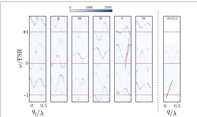
The spectra of the cavity modes reported infigures8and9are obtained by detecting the light of a laser at 1064 nm transmitted by the cavity while scanning the laser frequency for different positions of the membrane(s).
The last panel on the right offigure8is equal to the last offigure9and they report the results of the single membrane case. The slope of the corresponding black lines represents the maximum achievable single membrane optomechanical coupling strengthGsingmax 2p ´3.47 MHz nm-1. The other panels show the results with two membranes. In this case there are two degrees of freedom that can be varied,that is,the positions of the two membranes, q1and q2. Due to the design of our membrane-cavity, we can scan either the CoM, Q, for different values of the membrane distanceq=q2-q1,or q1for different positions of q2. Infigure8are reported
Figure 5. Experimental setup for characterizing the mechanical properties of the two membranes constituting the membrane-cavity.
A532 nmlaser is sent into a polarization-multiplexed Michelson interferometer. Thermal voltage noise of the two-membrane cavity
is revealed by homodyne detection of the reflected light. HWP denotes a half-waveplate, QWP a quarter-waveplate, and PBS a polarizing beam-splitter.
the spectra obtained by scanning the CoM, Q, for different values of the membrane distance q, as indicated by the lines A–F in figure2. The blue line on panel D corresponds to the blue circle infigure2, and it indicates the highest couplingGQmax2p ´5.67 MHz nm-1achieved in this case. It corresponds to an increase in the optomechanical coupling strength of a factor ~1.63 with respect to the single membrane case. Infigure9we report the spectra obtained by scanning the position q1for different position q2, as indicated by the lines I–VI in
Figure 6. Thermal noise measurement of the mechanical modes of the two membranes in a Michelson interferometer.(a) Thermal voltage noise(VSN) (green curve) with the experimental mechanical resonance peaks highlighted by vertical light-grey lines; red and blue top lines indicate the mechanical frequencies of rectangular membranes with nominal values for the stresss = 0.825 GPaand density r =3100 kg m-3, and best best-fit parameters for the side lengthsL( )=1.519 0.006 mm,L( )=1.536 0.006 mm
x1 y1 ,
andL( )=1.522 0.006 mm,L( )=1.525 0.006 mm
x2 y2 , respectively. The grey curve is the shot noise, while the black curve the
electronic noise.(b) Relative difference between experimental and fitted mechanical frequencies for the two membranes. (c) Quality factormof each mechanical mode.
Figure 7. Experimental setup for the measurements reported infigures8, and9. The light of a laser at1064 nmwavelength transmitted by an optical cavity of lengthL=90 mm containing the membrane sandwich of thicknessLm=104 nm, and distanceLc=24 mm
at rest, is revealed by a PIN photodiode(tr), while the frequency is scanned by applying a ramp signal (RAMP) to the piezo control of the laser. The positions of the two membranes are controlled by applying high voltage(HV) to the piezos, which move the CoM, Q, and the cavity length, q1.
figure2. The red line on panel V corresponds to the red circle infigure2, and indicates the highest achieved couplingG1max2p ´8.59 MHz nm-1. In this case the optomechanical coupling strength increases by a factor ~2.47, which is 9% lower than the expected one, given by equation(31). Such a discrepancy might be
attributed to an imperfect alignment of the two membranes.
Figure 8. Mode frequency shift normalized to the FSR, as a function of the CoM, Q, normalized to the wavelength, for different values of the distanceq=q2-q1as indicated by the lines A–F in figure2. Panel D shows the position of the highest achievable coupling
p ´
-
GQmax 2 5.67 MHz nm 1indicated by the solid blue line. For comparison the single membrane result is added as a dotted black
line, which represents the maximum achievable couplingG 2p ´3.47 MHz nm
-singmax 1, shown in the panel on the right.
Figure 9. Mode frequency shift normalized to the FSR, as a function of the membrane position q1, normalized to the wavelength, for
different values of the position q2, as indicated by the lines I–VI in figure2. Panel V shows the positions for the highest coupling
p ´
-
5. Cavity
finesse in the presence of the membrane-sandwich
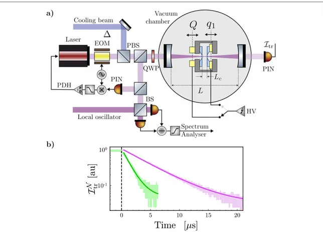
In the last set of experiments we placed the second membrane sandwich(the one made of Si N3 4membranes) in the same optical cavity offigure7(see also figure10(a)). Here we report on the analysis of the effects of the membranes on
the cavityfinesse. The finesse of the optical cavity, with and without the membrane sandwich, is determined by means of the ring-down technique,fitting the decay of the normalized transmitted intensity, tr, after the laser at 1064 nm is rapidly turned off. Infigure10(b) we show the ring-down results obtained for the empty cavity, and with the
membrane-sandwich placed within the optical cavity. For the former case, the best-fit decay time is t =0 4.790 m
0.002 s, which corresponds to an empty cavityfinesse 0=pt0c L=50 12525[27], while for the latter, t =1.365 0.001 s, corresponding to a cavitym finesse =14 287 13. Suchfinesse corresponds to a cavity intensity decay ratek=t-1=FSR ~2p´117 kHz, withFSR~2p´1.67 GHz. The observed reduction offinesse in the presence of the membrane-sandwich is much more significant than the one occurring in the case of a single membrane[24,29] and it can be ascribed to the imperfect alignment of the two membranes [20]. This
misalignment is responsible for an effective cavity loss1 d=1 -1 0( Fmqwdg qdif)2 2p50 ppm. Assuming a coefficient of finesseFm=4m (1-m)23, and a diffraction angle of the gaussian beam qdif =l pw03 mrad, withw0112 mm the beam waist of the cavity of our experiment, the misalignment angle qwdgbetween the two non-parallel membranes can then be estimated to be qwdg~ 30 radm . The membrane alignment could be improved either by using pairs of membranes assembled parallel to each other by means of spacers deposited on one of the chip, as implemented for example in the experiment of[20], or by replacing the single
Figure 10.(a) Experimental setup for studying cavity optomechanics with a two-membrane setup within a cavity. A laser probe beam, frequency modulated by an electro-optical modulator(EOM), impinges on the optical cavity. The reflected beam is split: one component is detected, demodulated and low-pass amplified for generating the Pound–Drever–Hall (PDH) error signal able to lock the laser to the cavity; the second component is analysed by homodyne detection in order to detect the mechanical motion. A further beam, the cooling beam, detuned byΔ from the cavity resonance, is turned on for engineering the optomechanical interaction, and in particular realize laser cooling of the mechanical modes. HWP denotes a half-waveplate, QWP a quarter-waveplate, BS a beam-splitter, and PBS a polarizing beam-splitter.(b) Cavity ring-down measurement for the evaluation of the cavity finesse. Light-violet data is the normalized transmitted intensity, tr, through the empty optical cavity; the solid violet line represents the best-fit with
decay time t0=4.790 0.002 sm, which corresponds to an empty cavityfinesse 0=pt0c L=50 12525. Light green data
refer to the case with the membrane-sandwich placed within the optical cavity; the solid green line is the best-fit with decay time
piezo, used for the scan of the membrane-cavity, with tilt stages with piezo control, which would allow for scanning as well as alignment of the membrane-cavity.
6. Tunable optomechanical coupling and laser cooling of the two membranes
Using the same setup of section5, wefinally studied the optomechanical properties of the system. First we show that the optomechanical interaction of the driven cavity mode with each membrane of the sandwich can be controlled and tuned by shifting their position along the cavity axis with the piezo controllers. The probe beam was locked to the optical cavity by means of a Pound–Drever–Hall technique and the thermal voltage spectral noise(VSN) of the two-membranes cavity is measured by homodyne detection of the light reflected by the optical cavity(see figure10(a)). The detected thermal (VSN) is shown in figure11, which clearly manifests the possibility to turn on and off the optomechanical interaction in a controlled manner by changing the position of each membrane(see figures11(a) and (b)) where only one of the two membranes is positioned in a place in
which it interacts with the cavity light. Infigure11(c) both membranes are instead coupled to the optical cavity.
For the lower frequency mode on the left(red) we measured wm1=2p´235.810 kHz,gm1=2p´1.64 Hz, while for the mode on the right(orange) we measured wm2=2p´236.580 kHz,gm2=2p´9.37 Hz. Such results are consistent with the measurements obtained with the interferometer(see figure6). In fact, we used a
probe beam with very low power, and as resonant as possible with a cavity mode in order to avoid any optomechanical effect, such as cooling or optical spring effect, taking into account that k~ ¯wm 2with w¯m=(wm1+wm2) 2. The corresponding measured single-photon optomechanical coupling rates
= Q
g0j G xj j j
zpf
, wherexjzpf = [ 2mjw( )mj]1 2is the zero point positionfluctuations of the jth mechanical mode, andΘjis the dimensionless transverse overlap between the jth mechanical mode and the optical cavity mode,[30] areg01=2p´0.30 Hzandg02=2p´0.28 Hz. These values are comparable to those achieved in a similar setup with a single membrane[27,31] because the two membranes were placed out of the region in the
q1, q2plane where the optomechanical coupling is enhanced due to interference(see figure2). Within this region the system was not stable enough and we did not carry out cavity optomechanics experiments.
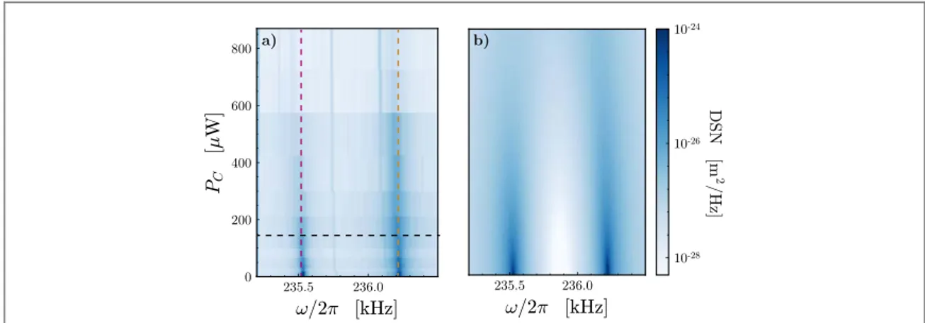
Finally we show that we can engineer the optomechanical interaction of both membranes with the optical mode by turning on an additional‘cooling’ beam with a variable detuning Δ with respect the cavity resonance. Here we focus on the case of red-detuned driving which resonantly enhances the beam-splitter interaction between the cavity mode and the mechanical modes and allows to cool the latter. We observe the simultaneous cooling[32] of the fundamental modes of the two distinct membranes. In figures12and13we report the measured displacement spectral noise(DSN) (left panels) as a function of the detuning Δ normalized to the
Figure 11. Thermal voltage(VSN) and displacement (DSN) spectral noise of the membrane sandwich obtained by homodyne detection of the light reflected by the optical cavity. (a) Only the membrane with lower frequency fundamental mode is coupled to the optical cavity.(b) Only the membrane with higher frequency fundamental mode is coupled to the optical cavity. (c) The fundamental modes of both membranes are coupled to the optical cavity. The green feature on the right indicates the beat note added for calibration. For the left red mode we determine: wm1=2p´235.810 kHz,gm1=2p´1.64 Hz, andg01=2p´0.30 Hz;and for
Figure 12. Laser cooling of the two membranes at low power.(a) Measured displacement spectral noise (DSN) as a function of the detuningΔ normalized to the mean mechanical frequency w¯m=(wm1+wm2) 2, for a cooling input powerPC=130 Wm , k=2p´83 kHz, and g0as infigure11. The red and orange dashed lines indicate the mechanical frequencies with no cooling.
(b) Theoretical prediction with parameters given in figure11.
Figure 13. Laser cooling of the two membranes at high power.(a) Measured displacement spectral noise (DSN) as a function of the detuningΔ normalized to the mean mechanical frequency w¯m=(wm1+wm2) 2, for a cooling input powerPC=380 Wm , and k=2p´83 kHz. The red and orange dashed lines indicate the mechanical frequencies with no cooling.(b) Theoretical prediction with the following parameters: wm1=2p´235.950 kHz,gm1=2p´1.64 Hz, andg01=2p´0.12 Hz;and for the right blue
mode: wm2=2p´236.750 kHz,gm2=2p´9.37 Hz, andg02=2p´0.22 Hz. Note the less effective optomechanical cooling
on the left mode due to lower optomechanical coupling, and also the frequency shift in the moderate resolved-side-band limit.
Figure 14. Laser cooling of the two membranes at constant detuning.(a) Measured displacement spectral noise (DSN) as a function of the cooling beam power PC. The red and orange dashed lines indicate the mechanical frequencies with no cooling.(b) Theoretical
mean mechanical frequencyw¯m, and compare it with the corresponding theoretical prediction(right panels). In
figure12we use a lower power of the cooling beam with respect to that used infigure13, but in both cases the agreement is very good. Infigure14instead we report the DSN as a function of the cooling beam power PC, at a fixed detuningD ~ ¯wm.
7. Conclusion
We studied the optomechanical behaviour of a driven Fabry–Pérot cavity containing a two-membrane sandwich. From the cavity mode frequency shift as a function of the membrane positions, we derived a∼2.47 gain in the optomechanical coupling strength with respect to the single membrane case. This is obtained when the two membranes are positioned to form an inner cavity resonant to the drivingfield. We also showed the capability of the system to be tuned on demand, and the simultaneous optical cooling of the fundamental modes of the two distinct membranes. Such a configuration has the potential to enable cavity optomechanics in the strong single-photon coupling regime[3–5], as well as to study the nonlinear dynamics and synchronization of
two distinct nano-mechanical resonators by means of an optical link[12–16].
Acknowledgments
Authors thank M Rossi, N Kralj, A Borrielli, G Pandraud, and E Serra for the single membrane spectrum obtained in the alignment procedure of the optomechanical system reported in[27,28,31]. The authors also
thank R Gunnella for the use of the spectrometer, and R Tossici for opticalfiber patches. PP acknowledges support from the European Union’s Horizon 2020 Programme for Research and Innovation under grant agreement No. 722923(Marie Curie ETN—OMT). We also acknowledge the support of the European Union Horizon 2020 Programme for Research and Innovation through the Project No. 732894(FET Proactive HOT).
ORCID iDs
Paolo Piergentili https://orcid.org/0000-0003-2125-4766
Mateusz Bawaj https://orcid.org/0000-0003-3611-3042 Stefano Zippilli https://orcid.org/0000-0001-5963-4823 Nicola Malossi https://orcid.org/0000-0002-5729-3399
Riccardo Natali https://orcid.org/0000-0001-9348-6895 David Vitali https://orcid.org/0000-0002-1409-7136
Giovanni Di Giuseppe https://orcid.org/0000-0002-6880-3139
References
[1] Bhattacharya M and Meystre P 2008 Phys. Rev. A78 041801
[2] Hartmann M J and Plenio M B 2008 Phys. Rev. Lett.101 200503
[3] Xuereb A, Genes C and Dantan A 2012 Phys. Rev. Lett.109 223601
[4] Xuereb A, Genes C and Dantan A 2013 Phys. Rev. A88 053803
[5] Li J, Xuereb A, Malossi N and Vitali D 2016 J. Opt.18 084001
[6] Nair B, Xuereb A and Dantan A 2016 Phys. Rev. A94 053812
[7] Li J, Li G, Zippilli S, Vitali D and Zhang T 2017 Phys. Rev. A95 043819
[8] Ludwig M and Marquardt F 2013 Phys. Rev. Lett.111 073603
[9] Weaver M J, Buters F, Luna F, Eerkens H, Heeck K, de Man S and Bouwmeester D 2017 Nat. Commun.8 824
[10] Heinrich G, Ludwig M, Qian J, Kubala B and Marquardt F 2011 Phys. Rev. Lett.107 043603
[11] Holmes C A, Meaney C P and Milburn G J 2012 Phys. Rev. E85 066203
[12] Zhang M, Wiederhecker G S, Manipatruni S, Barnard A, McEuen P and Lipson M 2012 Phys. Rev. Lett.109 233906
[13] Bagheri M, Poot M, Fan L, Marquardt F and Tang H X 2013 Phys. Rev. Lett.111 213902
[14] Agrawal D K, Woodhouse J and Seshia A A 2013 Phys. Rev. Lett.111 084101
[15] Matheny M H, Grau M, Villanueva L G, Karabalin R B, Cross M C and Roukes M L 2014 Phys. Rev. Lett.112 014101
[16] Zhang M, Shah S, Cardenas J and Lipson M 2015 Phys. Rev. Lett.115 163902
[17] Baker C, Hease W, Nguyen D T, Andronico A, Ducci S, Leo G and Favero I 2014 Opt. Express22 14072–86
[18] Balram K C, Davanço M, Lim J Y, Song J D and Srinivasan K 2014 Optica1 414–20
[19] Meenehan S M, Cohen J D, Gröblacher S, Hill J T, Safavi-Naeini A H, Aspelmeyer M and Painter O 2014 Phys. Rev. A90 011803
[20] Nair B, Naesby A and Dantan A 2017 Opt. Lett.42 1341–4
[21] Bhattacharya M, Uys H and Meystre P 2008 Phys. Rev. A77 033819
[22] Jayich A M, Sankey J C, Zwickl B M, Yang C, Thompson J D, Girvin S M, Clerk A A, Marquardt F and Harris J G E 2008 New J. Phys.10 095008
[24] Serra E, Bawaj M, Borrielli A, Di Giuseppe G, Forte S, Kralj N, Malossi N, Marconi L, Marin F, Marino F, Morana B, Natali R, Pandraud G, Pontin A, Prodi G A, Rossi M, Sarro P M, Vitali D and Bonaldi M 2016 AIP Adv.6 065004
[25] Luke K, Okawachi Y, Lamont M R E, Gaeta A L and Lipson M 2015 Opt. Lett.40 4823–6
[26] Bawaj M, Biancofiore C, Bonaldi M, Bonfigli F, Borrielli A, Di Giuseppe G, Marconi L, Marino F, Natali R, Pontin A, Prodi G A, Serra E, Vitali D and Marin F 2015 Nat. Commun.6 7503
[27] Rossi M, Kralj N, Zippilli S, Natali R, Borrielli A, Pandraud G, Serra E, Di Giuseppe G and Vitali D 2017 Phys. Rev. Lett.119 123603
[28] Kralj N, Rossi M, Zippilli S, Natali R, Borrielli A, Pandraud G, Serra E, Giuseppe G D and Vitali D 2017 Quantum Sci. Technol.2 034014
[29] Wilson D J, Regal C A, Papp S B and Kimble H J 2009 Phys. Rev. Lett.103 207204
[30] Gorodetsky M L, Schliesser A, Anetsberger G, Deleglise S and Kippenberg T J 2010 Opt. Express18 23236–46
[31] Rossi M, Kralj N, Zippilli S, Natali R, Borrielli A, Pandraud G, Serra E, Di Giuseppe G and Vitali D 2018 Phys. Rev. Lett.120 073601