Problems in measurement of mechanical loads in wind turbines: bending/torsional moments by strain gage bridges and torque by optical transducer

(1)

Università Politecnica delle Marche

Scuola di Dottorato di Ricerca in Scienze dell’Ingegneria Corso di Dottorato in Ingegneria Industriale ---

Problems in measurement of mechanical

loads in wind turbines: bending/torsional

moments by strain gage bridges and torque

by optical transducer

Ph.D. Dissertation of:

Ing. Matteo Bezziccheri

Supervisor:

Prof. Nicola Paone

Assistant Supervisor:

Dr. Christopher James Crabtree

Ph.D. Course coordinator:

Prof. F. Mandorli

(2)

Università Politecnica delle Marche

Dipartimento di Ingegneria Industriale e Scienze Matematiche DIISM

(3)

Dedicated to

(4)

(5)

Abstract

The analysis of mechanical loads today plays a crucial role in the certification of wind turbines (WT). Similarly, mechanical loads measurement is relevant for condition monitoring of wind turbines; as rapid detection of abnormal loads can help preventative maintenance with a direct impact on machine operation and maintenance (O&M) costs. This thesis discusses the complexity of measuring mechanical loads on HAWT wind turbines.

The most important mechanical loads on a wind turbine are bending and torsional moments that are usually measured through strain gage full bridges, as recommended by the standard IEC 61400-13.

This thesis at first discusses the guidelines for the design the strain gage measurement chain, comparing the possible configurations of the full strain gage bridges (parallel or T), as well as the possible electrical connection (4 wires or 6 wires) and showing a typical configuration of the network of DAQ systems. Next, a comparison among the different calibration procedures, analytical, external loads and gravity, is presented. The gravity calibration is often the recommended solution. This work presents static-dynamic models, which allow to calibrate the full strain gage bridges using its own imbalanced masses, and comments on the attainable range of calibration, which is rather limited with respect to expected load range in operation. For each model, an uncertainty analysis of the calibration process will be presented, according to the ISO/IEC Guide 98-3: 2008 "Guide to the Expression of Uncertainty in Measurement".

Even if measurement should take place in isothermal effects, this is not always the case in real world practice. Therefore, the thermal effects on strain gage bridges are also discussed, putting into evidence its influence on calibration and signal uncertainty both for full bridges in T configuration and in parallel configuration. Among the strain gage measurements that can be performed on wind turbines, the torque measurement on the shaft is often the most uncertain because it is affected by strong crosstalk phenomena. However, many studies have shown that an accurate torque measurement can provide much information about the WT’s health and it has been shown to be a successful method for detecting faults in the main drive train components. Although WT torsional effects are important, torque measurement on wind turbine shaft is a complex task today; the available solutions are uncertain (like strain gage) or invasive (like inline torque sensor).

This thesis, in its second part, analyses a novel, contactless torque measurement system consisting of two shaft-mounted zebra tapes and two optical sensors mounted on stationary rigid supports. Unlike conventional torque measurement methods, the system, initially proposed by Durham University, does not require

(6)

costly embedded sensors or shaft-mounted electronics. The performance of the system has been analyzed experimentally on a small scale laboratory test bench under both static and dynamic conditions; the technique has been implemented using two different signal processing methods, rising edge and cross-correlation approaches. The results show good agreement with reference measurements from an in-line, invasive torque transducer. The uncertainty according to the ISO/IEC Guide 98-3: 2008 "Guide to the Expression of Uncertainty in Measurement" is shown to be ±0.3% and ±0.8% of full-scale torque for the rising edge and cross-correlation approaches, respectively. Finally, a feasibility analysis and a system scale-up design for two typical WTs with different shaft configurations, 60 kW wind turbine with gearbox and 3 MW wind turbine with direct drive train, has been performed. The expected uncertainty for the two solutions is 2.0% and 0.5%, respectively.

(7)

Sommario

L’analis di carichi meccanici svolge oggi un ruolo cruciale nella certificazione di turbine eoliche (WT). Allo stesso modo, la misura dei carichi meccanici è rilevante per monitorare le condizioni di turbine eoliche; poiché, tramite un rilevamento rapido di carchi insoliti, è possibile adottare una manutenzione preventiva con un impatto diretto sulle spese di funzionamento e manutenzione (O&M) della macchina. Questo lavoro discute la complessità di misurare carichi meccanici su grandi turbine eoliche.

I carichi meccanici di maggior rilievo su una turbina eolica sono momenti flettenti e torcenti che, in accordo con lo standard IEC 61400-13, è consigliabile misurare attraverso ponti estensimetrici interi.

Questa tesi all’inizio discute le linee guida per la progettazione della catena di misura estensimetrica, confrontando le possibili configurazioni dei ponti estensimetrici adottabili (parallelo o T), i collegamenti elettrici adottabili (4 fili o 6 fili) e mostrando una tipica configurazione della rete dei sistemi di acquisizione DAQ. A seguire, viene mostrato un confronto tra le diverse possibili procedure di calibrazione: analitica, carichi esterni e squilibri propri. La procedura che sfrutta gli squilibri propri è la soluzione spesso consigliata. Il lavoro presenta modelli statici-dinamici, che consentono di calibrare i ponti estensimetrici usando gli squilibri di massa propri, e commenta gli intervalli di calibrazione raggiungibili per una tipica turbina, che sono piuttosto limitati rispetto ai carichi massimi attesi in esercizio. Per ciascun modello sarà poi presentata una analisi di incertezza del processo di calibrazione, in accordo con la ISO/IEC Guide 98-3:2008 “Guide to the Expression of Uncertainty in Measurement”.

Anche se la calibrazione dovrebbe avvenire in condizione isotermiche, questa condizione nella pratica non può essere sempre verificata. Pertanto, vengono discussi gli effetti termici sui ponti estensimetrici, mettendo in evidenza lo loro influenza sull'incertezza di calibrazione e sull’incertezza del segnale sia per ponti in configurazione T che in configurazione parallela.

Tra le misure estensimetriche eseguite su turbine eoliche quella della misura della coppia sull’albero è spesso la più incerta, poiché affetta da forti fenomeni di crosstalk. Tuttavia, un segnale di coppia accurato può fornire molte informazioni sul stato di salute della turbina eolica, studi hanno infatti dimostrato che una analisi dei segnali di coppia permettono di rilevare guasti nei componenti principali del sistema di trasmissione. Nonostante ciò, la misura della coppia sugli alberi di turbine eoliche è ad oggi complessa; le soluzioni di misura adottabili sono incerte (come gli estensimetri) o invasive (come i torsiometri in linea).

(8)

Questa tesi nella seconda parte analizza una tecnica di misura della coppia innovativa e senza contatto costituita da due nastri zebrati montati sull’albero e due sonde ottiche su un supporto rigido non rotante. A differenza dei metodi convenzionali di misura della coppia, il sistema, inizialmente proposta dall’Università di Durham, non richiede sensori costosi o il montaggio di elettroniche sull’albero. Le prestazioni del sistema proposto sono state analizzate in un piccolo banco prova da laboratorio durante condizioni statiche e dinamiche; la tecnica è stata implementata usando due metodi di elaborazione del segnale, approccio rising edge e approccio cross-correlation. I risultati mostrano una buona corrispondenza con le misure di riferimento eseguite attraverso un torsiometro in linea. L'incertezza calcolata in accordo con la ISO GUM (Guide to the Expression of Uncertainty in Measurement) è dello ± 0,3% e ± 0,8% della coppia massima misurabile, rispettivamente per gli approcci del rising edge e cross-correlation. Infine, è presentata una analisi di fattibilità e un disegno di scala del sistema per due turbine eoliche con una diversa configurazione dell’albero, turbina eolica da 60kW con sistema di trasmissione con ingranaggio e turbina eolica da 3 MW con sistema di trasmissione ad azionamento diretto. L’incertezza attesa sulla misura della coppia per le due soluzioni è rispettivamente del 2.0 % e 0.5%.

(9)

Acknowledgements

Over the three years from November 2014, many people have assisted me in completing the work described in this thesis and I am grateful to them all.

In particular:

• My PhD supervisor, Prof. Nicola Paone, whose academic guidance and encouragement has been a constant source of motivation. I appreciate all the fruitful discussions and feedback received to make my PhD experience productive and stimulating. His constant support and enlightening guidance in the development and completion of this thesis.

• The technicians at Università Politecnica delle Marche. Particularly, Luca Violini, Engr. Claudio Santolini and Piersavio Evangelisti for their patience, motivation, enthusiasm, and immense knowledge. Their guidance helped me in all the time of research and writing of this thesis.

• Prof. Chris Crabtree and Dr. Donatella Zappalà that gave me the opportunity to work with them and to share the project that has been presented in Chapter 6.

• All those, past and present, from within the Mechanical and Thermal Measurement Group at DIISM who have provided an excellent working atmosphere. In particular, Prof. Enrico Primo Tomasini, Prof. Paolo Castellini, Prof. Gianmarco Revel, Prof. Milena Martarelli, Prof. Lorenzo Scalise and all researchers and PhD students.

• Prof. Renato Ricci for his support in dealing with aerodynamic issues. • Prof. Lucio Demeio and Prof. Ferrante for their assistance in dealing

uncertainty analysis.

• Dr. Matteo Claudio Palpacelli for his assistance in developing calibration models.

(10)

Publications

Peer reviewed publications Journal papers

1. Bezziccheri M., Castellini P., Evangelisti P., Santolini C. and Paone N. (2017). Measurement of mechanical loads in large wind turbines: problems on calibration of strain gage bridges and analysis of uncertainty. Wind Energy, pp. 1–14, doi: https://doi.org/10.1002/we.2136.

2. Zappalà D., Bezziccheri M., Crabtree C.J. and Paone N. (2017). Non-intrusive torque measurement for rotating shafts using optical sensing of zebra-tapes. Measurement Science and Technology, under review.

Conference proceedings

1. Bezziccheri M., Castellini P., Evangelisti P., Santolini C., Paone N. (2015). Uncertainty associated with strain gauge measurements on wind turbines.

EWEA Annual Event, European Wind Energy Association, (Paris from 17 to

20 November 2015) abstract available at

https://www.ewea.org/annual2015/conference/submit-an-abstract/pdf/2911067515994.pdf.

Posters

1. Zappalà D., Bezziccheri M., Crabtree C.J., Paone N., Rendell S. (2016). Wind turbine non-intrusive torque monitoring. SUPERGEN Wind General

(11)

List of Figures

Figure 1 World energy consumption by country grouping, 2012–40 (quadrillion Btu)

[1] ... 2

Figure 2 Total world energy consumption by energy source, 1990–2040 (quadrillion Btu) [1] ... 3

Figure 3 Levels of carbon dioxide in the atmosphere and the Antarctic temperature over the past 800,000 years (Graphs by Robert Simmon, using data from Lüthi et al., 2008, and Jouzel et al., 2007.) ... 3

Figure 4 Atmospheric CO2 levels (Green is Law Dome ice core, Blue is Mauna Loa, Hawaii) and Cumulative CO2 emissions (CDIAC) ... 4

Figure 5 Expected Renewable Energy Standard deployments in Member States and 2020 Renewable Energy Standard targets ... 5

Figure 6 Global cumulative installed wind capacity 2001-2016. Source GWEC [49] 7 Figure 7 Global cumulative wind power capacity. Source GWEC [41]. ... 7

Figure 8 Distribution of wind energy density (GWh/km2_{)in europe for 2030 (80 m} hub height onshore, 120 m hub height offshore)[38] ... 9

Figure 9 Distribution of full load hours in Europe (80 m hub height on shore, 120 m hub height offshore)[38] ... 9

Figure 10 Worldwide installed offshore wind capacity[42] ... 10

Figure 11 International breakdown of installed offshore wind capacity [42] ... 11

Figure 12 Crucial parts of a HAWT ... 12

Figure 13 Box plot representation of rotor diameters of onshore wind turbines annually installed [20]. Sorce:JRC data ... 13

Figure 14 Box plot representation of hub heights of onshore wind turbines annually installed [20]. Source: JRC database ... 14

Figure 15 Box plot representation of rated power of onshore wind turbines annually installed [20]. Source: JRC database ... 14

Figure 16 Wind turbine types according to drive train configuration [20] ... 16

Figure 17 Evolution of the share of installed capacity by wind turbine configuration [20]. Source: JRC database ... 16

Figure 18 Wind power, turbine power, and operating regions for an example 5 MW turbine[25] ... 18

Figure 19 Evolution of power control approach of onshore wind turbines annually installed. Source: JRC database ... 20

Figure 20 Evolution of the share of onshore installed capacity by IEC wind classes. Source: JRC database ... 21

Figure 21 Wind turbine design process [53][51] ... 27

Figure 22 Modules of Type Certification [51] ... 31

Figure 23 Modules of Project Certification [51] ... 33

(16)

Figure 25 Cost of electricity by region and technology and their weighted average

2013/2014[74] ... 42

Figure 26 CoE ranges by renewable power generation technology, 2014 and 2025 [74] ... 43

Figure 27 Influence of the maintenance strategy on asset condition [77] ... 44

Figure 28 Costs associated with the three maintenance strategies [69] ... 44

Figure 29 Distribution of normalised failure rate by sub-system and subassembly for WTs of multiple manufactures from the ReliaWind survey [79] ... 45

Figure 30 Distribution of normalised downtime by sub-system and subassembly for WTs of multiple manufactures from the ReliaWind survey [79] ... 46

Figure 31 WT failure rate & downtime per failure from results for onshore WTs from 3 surveys (WMEP, LWK &Scandinavian) including >24000 turbine-years of operation [81] ... 46

Figure 32 Stop rate and downtime data from Egmond aan Zee WF over 3 years [83]. ... 47

Figure 33 Distribution of failure rates between different WT models [84] ... 48

Figure 34 Correlation between failure rate & WEI [86] ... 48

Figure 35 Structural health and condition monitoring of a wind turbine [89] ... 50

Figure 36 Distribution of advance-detection periods for faults detected based on SCADA data (Physical-Model approach) in the validation study [90] ... 51

Figure 37 Framework of the interaction between condition monitoring, diagnosis, prognosis and maintenance systems, according to [94] and [69]. ... 53

Figure 38 Nacelle co-ordinate system [50] ... 65

Figure 39 Hub co-ordinate system [50] ... 65

Figure 40 Typical full bridges used in wind turbine type testing for bending moments [145] ... 67

Figure 41 Typical full bridge used in wind turbine type testing for torsional moments ... 67

Figure 42 Eight-wire and four-wire connection of full-bridge circuit ... 67

Figure 43 Six-wire connection of full-bridge circuit ... 68

Figure 44 Tower top bending moment before reinstallation ... 69

Figure 45 Tower top bending moment after reinstallation ... 69

Figure 46 – The network of DAQ systems installed in the turbine ... 70

Figure 47 Scheme for Analytical calibration on the strain gauge bridges for measuring bending moments ... 73

Figure 48 Scheme for Analytical calibration on the strain gauge bridges for measuring torque ... 74

Figure 49 Blade and Shaft moments genereted by external mass hangs to the blade ... 75

Figure 50 Tower top and tower bottom moments genereted by pulling the tower by ropes ... 75

(17)

Figure 51 Scheme of analytical calibration: reference input load is based on known

unbalanced masses and turbine modelling [156] ... 75

Figure 52 Blade bending moments generated by blade rotation over 360 ° [156] 76 Figure 53 Reference systems and characteristic angles [156] ... 78

Figure 54 Development of known bending moments on the shaft [156] ... 80

Figure 55 Development of bending moments known exploiting the imbalance of mass induced by the system nacelle, hub and rotor [156] ... 81

Figure 56 Signals during a series of rotor rotation under no-wind show cross-talk between channels ... 83

Figure 57 – Generator efficiency vs. angular speed and power ... 85

Figure 58 Linear regression through the offsets derived from the different calibration runs [50] ... 89

Figure 59 Calibration data for Mbe [156]. ... 90

Figure 60 Thermal image of the tower top ... 94

Figure 61 Thermal influence of the power converters on the strain gages on the tower bottom ... 94

Figure 62 Thermal influence caused by solar radiation on full bending bridge at tower bottom in parallel configuration ... 98

Figure 63 Apparent electric voltage expected in output from a bending strain gage bridge in parallel configuration glued on steel ... 100

Figure 64 Thermal data influenced by the thermal drift ... 102

Figure 65 Thermal data not influenced by the thermal drift ... 102

Figure 66 Covariance ... 102

Figure 67 Operating principle of the non-intrusive torque measurement system ... 108

Figure 68 Schematic diagram of the torque test rig ... 110

Figure 69 Main components and instrumentation of the torque test rig ... 110

Figure 70 Solid shaft layout and location of the two zebra tapes ... 111

Figure 71 Detail of the contactless shaft torque measurement system ... 111

Figure 72 Optical probe response to zebra tape ... 114

Figure 73 Data processing flow diagram ... 115

Figure 74 Signal initialisation ... 116

Figure 75 Flicker filter ... 117

Figure 76 Phase shift estimation through the rising edge detection approach ... 119

Figure 77 Phase shift estimation through the cross-correlation approach ... 119

Figure 78 Calibration curve: Rising edge detection approach ... 122

Figure 79 Calibration curve: Cross-correlation approach ... 122

Figure 80 Effect of sensor to shaft distance variation on the optical probe output ... 125

(18)

Figure 82. PDF propagation of the four independent input quantities to provide the

PDF of (adapted from [184]). ... 127

Figure 83. PDF propagation of K, n and Δt to provide the PDF of Trotor through the zebra tape torque meter model (adapted from [184]). ... 129

Figure 84 Optical system speed and torque measurement under steady state conditions: (a) and (c) 1700 rpm and 4 Nm; (b) and (d) 1900 rpm and 10 Nm .... 131

Figure 85 Optical system speed (a) and torque (b) measurements under sharp step torque changes ... 132

Figure 86 Optical system speed (a) and torque (b) measurements under torque varying at three different frequencies (0.17 Hz, 0.30 Hz and 0.63 Hz) ... 133

Figure 87 60 kW wind turbine and drivetrain with gear box ... 135

Figure 88 Shaft of 60 kW wind turbine and drivetrain with gearbox ... 136

Figure 89 Multi megawatt wind turbine and direct drivetrain [188] ... 137

(19)

List of Tables

Table 1 Projected deployment and deviation from planned EU technology

deployment 2014 and 2020 ... 6

Table 2 Capacity scenarios per country (MW)[39]... 8

Table 3 Wind turbine classes [37] ... 21

Table 4 Status of IEC standard and certification procedure [52] ... 26

Table 5 Design Load Cases (DLCs) [37] ... 29

Table 6 Wind turbine standards for prototype tests ... 32

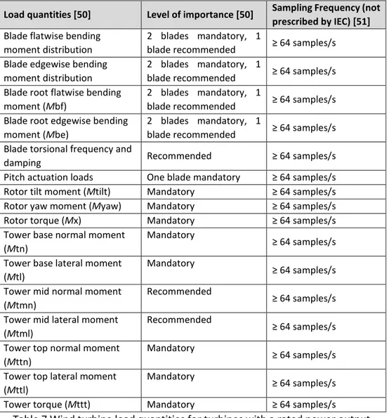
Table 7 Wind turbine load quantities for turbines with a rated power output greater than 1500 kW and rotor diameter greater than 75 m ... 35

Table 8 Meteorological quantities ... 36

Table 9 Wind turbine operation quantities... 36

Table 10 OM cost in North America and Europe [73],[74] ... 42

Table 11 Minimum sensor requirements for vibration-based CM according to the GL Certification Guideline 2013 [103] [77] ... 55

Table 12 Overview of commercially available sensors for oil condition monitoring, according to [77] ... 56

Table 13 Wind turbine load quantities for turbines with a rated power output greater than 1500 kW and rotor diameter greater than 75 m, according to IEC 61400 – 13 Edition 2015 [50]. ... 64

Table 14 Summary of suitable calibration methods [50]. ... 71

Table 15 Combined standard uncertainty for ratios, RUs, between 1 and 10 [156]. ... 91

Table 16 Values and uncertainties of all bending moments [156] ... 93

Table 17 Uncertainty of all bending moments [156] ... 93

Table 18 Features of the experimental zebra tape. ... 113

Table 19 Parameters of the two calibration curves and relative Type A uncertainty, _ ... 124

Table 20 Measurement system model equations. ... 126

Table 21. Uncertainties and sensitivity analysis of the quantities contributing to ∆ . ... 128

Table 22. Uncertainties and sensitivity analysis of the quantities contributing to . ... 129

Table 23. Torque meter system Type B expanded uncertainty, uMCM. ... 130

Table 24 Expected shaft torque for 60 kW wind turbine and drivetrain with gearbox ... 136

Table 25 Technical data of 42CrMo4 steel ... 137

(20)

List of Abbreviations

ABB Asea Brown Boveri

ANN Artificial Neural Networks

APC Active Power Control

ASC Active Stall Control

CM Condition Monitoring

CMS Condition Monitoring System

DAQ Data AcQuisition

DFIG Double Fed Induction Generator

DLCs Design Load Cases

EEA Europian Enviroment Agency

EESG Electrically Excited Synchronous Generator

EN European Standard

EU European Union

FEM Finite Element Method

GL Guideline

GPIB General Purpose Interface Bus

GUM Guide to the Expression of Uncertainty in Measurement GWEC Global Wind Energy Council

HAWT Horizontal Axis Wind Turbine

IEC International Electrotechnical Commission IEEE Institute of Electrical and Electronic Engineers IPC Individual Pitch Control

IRENA International Renewable Energy Agency ISO International Organization for Standardization

JRC Joint Research Centre

LWK Landwirtschaftskammer Schleswig-Holstein

MCM Monte Carlo Method

MCSA Motor Current Signature Analysis

MLCs Measurement Load Cases

NI National Instruments

NREAPs National Renewable Energy Action Plans Initialized signal of the k-th optical probe Signal of the k-th optical probe

O&M Operations & Maintenance PDF Probability Density Function

PMSG Permanent Magnet Synchronous Generators PSC Passive Stall Control

SAW Surface Acoustic Wave

(21)

SCIG Squirrel Cage Induction Generators SHM Structural Health Monitoring

UNI Italian Organization for Standardization VAWT Vertical Axis Wind Turbine

VIs Virtual Instruments

WECSs Wind Energy Conversion Systems

WEI Wind Energy Index

WMEP Wissenschaftlichen Mess und Evaluierungsprogramm WRIG Wound-Rotor Induction Generator

(22)

Nomenclature

A Swept area of the rotor [m2_]

AB

Distance between the application section of the strain gages on the blade and the rotation axis of the shaft

[m]

AE Annual Energy production [kWh]

AGb

Distance between the application section of the strain gages and the center of gravity of the part of the blade to the right of the strain gages

[m] aj Half-width tolerance of xj

Av Availability

bi Ordinate at the origin of the calibration line of the i-th bridge

C Shaft damping coefficient kg m

s rad # Ca Moment of the Aerodynamic Load on the blade [Nm]

CoE Cost of Energy €

kWh Cp Wind turbine power coefficient

De

Outer diameters in the section of application of the

strain gauges [m]

&'() '*_ +,- Desired combined standard uncertainty [Nm]

Di

Inner diameters in the section of application of the

strain gauges [m]

E Young modulus of the measurement object [Pa]

e Excitation voltage of the strain gage bridge [V] e0 Electric output voltage of the strain gage bridge [mV] '

0,-'

Ratio between electric output and excitation voltage of the i-th strain gage bridge

'12345678

' Apparent electric voltage due to thermal effects E Young’s modulus in the section of application of the

strain gages [Pa]

EGc

Distance between the strain gages position and center of gravity of the part of shaft to the right of the strain gages

[m] EGr Distance between the strain gages section and

center of gravity of the system; rotor+hub [m] 9: Sample frequency of the shaft torque signal [Hz]

ff Frequency of failure 1

(23)

fOP Sampling frequency of the optical probe signal [Hz]

FRC Fixed Charge Rate [€]

g Acceleration of gravity ?( @

A-( ) Probability Density Function of the i-th quantities

G Shear modulus of the measurement object [Pa]

Gb Center of gravity of the blade

h Number of sample for covariance analysis

Ib Inertia matrix of the blade [kg m2_]

Ic Inertia matrix of the part of shaft to the right of the

strain gages [kg m2]

ICC Initial Capital investment Cost [€]

Ir Inertia matrix of the system; rotor+hub [kg m2_]

Is Inertia of the shaft [kg m2]

Js Shaft polar moment of inertia of the shaft [m4]

K Shaft torsional stiffness E

*

k Gauge factor

kp Covarage factor in uncertainty analysis

L Distance between the two optical probes [m]

LRC Levelized Replacement Cost [€]

mi Slope of the calibration line of the i-th bridge

E mb Mass of the part of the blade to the right of the

strain gages [kg]

mc Mass of the part of shaft to the right of the strain

gages [kg]

Mbe Blade root edgewise bending moment [Nm]

Mbf Blade root flatwise bending moment [Nm]

Mimax Expected design loads of the i-th moment [Nm]

Mi Mi-th moment [Nm]

mn Massa of the system nacelle, hub and rotor [kg]

mr Mass of the system rotor and hub [kg]

MTBF Mean Time Between Failures [h]

Mtl Tower base lateral bending moment [Nm]

Mtml Tower mid lateral bending moment [Nm]

Mtmn Tower mid normal bending moment [Nm]

Mtn Tower base normal bending moment [Nm]

MTTF Mean Time To Failure [h]

Mttl Tower top lateral bending moment [Nm]

Mttn Tower top normal bending moment [Nm]

(24)

n Shaft rotational speed [rpm] OGn Distance between tower axis and the center of

gravity of the system nacelle, hub and rotor [h]

OM Annual Operation and Maintenance cost €

kWh

P Zebra tape period [m]

Pa Available power in the wind [W]

G8_7 Electric active power output from the wind turbine [W]

Pmin Minimum zebra tape period [m]

ppr Number of pulses per shaft revolution pprmax Maximum allowable number of pulses per

revolution

Pt Energy extract from the wind turbines [W]

R Strain gage's resistance [Ω]

r Shaft radius [m]

Re Outer radius in the section of application of the

strain gauges [m]

Ri Inner radius in the section of application of the

strain gauges [m]

Rm Mean radius in the section of application of the

strain gauges [m]

H_I Coefficient of determination

Ru Ratio between desired combined uncertainty and

uncertainty of the reference moment

J Cross-correlation (_K4LMN 4 O Standard deviation of 4LMN 4 (PN Standard deviations of bi (6N Standard deviations of mi _E

(Q Standard deviations of shaft rotational speed [rpm] (R Standard deviations of shaft torsional stiffness, K E_*

(,N Standard deviation of Mi [Nm]

SL Pre-set threshold level of the trigger [V]

(S Standard deviation of xj

(TULVLU Standard deviation of Trotor [Nm]

(WU Standard deviation of X5 [rad]

Ta Force of the Aerodynamic Load on the blade [Nm]

(25)

Tmean Mean temperature of the bridge [°C]

tp Start time of the initialize signals [s]

Trotor Shaft torque [Nm]

Trotor-max Maximum shat torque expected during operation [Nm]

Trotor_RANGE Measuring shaft torque range [Nm]

Ts Stran gage operating temperature minus strain

gage calibration temperature (typically 20 °C) [°C] _` Uncertainty of aP 1 °C _b Uncertainty of a6 1 °C _U Uncertainty of a5 _°C1

+,- Combined standard uncertainty of each Mi moment [Nm]

G Uncertainty of E [Pa]

Uncertainty of k

,:78-P572-0Qc- Uncertainty of the reference moment _d

:78-P572-0Qc- [Nm]

u,+, Uncertainty obtained by applying the MCM [Nm]

fb Uncertainty of Rm measurement [m]

(TJh, T j) Covariance of T13 and T24 measurements [°C] klm and kno Uncertainty of T13 and T24 measurements [°C]

pq Uncertainty of xj

ɛst Uncertainty of ɛuf

:78_,N Calibration uncertainty of Mi [Nm]

u-v_,N Signal uncertainty of Mi [Nm]

2_,N Total standard uncertainty of Mi [Nm]

xj j-th parameter used in calibration model

XT Switching distance of the optical probe [m]

α Tilt angle of the nacelle [°]

αb

Thermal expansion coefficient of the measurement object

1 °C

αm

Thermal expansion coefficient of the strain gage grid material

1 °C

αr

Temperature coefficient of the electrical resistance of the strain gage grid foil

1 °C

β Blade pitch [°]

ΔR Variation of the strain gage's resistance [Ω] ∆ Temperature difference between adjacent strain _{gages of the bridge} [°C]

(26)

∆tr

Time shift between rising edge of pulse trains

evaluated using the rising edge method [s] ∆www5xyz Eight-point averaged time shift evaluated using the _{rising edge method} [s] ∆ :xyz Time shift per zebra tape pulse evaluated using the _{cross correlation method} [s]

δd Displacement between pulse centre of two optical

probes signal [s]

δtf Displacement between falling edge of two optical

probes signal [s]

δtr Displacement between rising edge of two optical

probes signal [s]

{X5 Resolution on X5 estimation [rad]

ɛ- Strain measured by i-th strain gage

εsL Apparent strain due to thermal effects: linear error

ɛuf Apparent strain due to thermal effects: residual _error ɛuTYT Apparent strain due to thermal effects: overall _error

η Drive train and generator efficiency

θ Rotor azimuth [°]

θa Absolute angular shift between two optical probes

signal [rad]

X7_:xyz Shaft absolute angular shifts evaluated using the _{cross correlation method} [rad] θa,0 Apparent angular shift between two optical probes

signal [rad]

X7_5x yz Shaft absolute angular shifts evaluated using the _{rising edge method} [rad]

X|}88s~•€• Maximum measurable shaft torsion angle [rad]

θmax

Maximum torsion angle of the shaft expected

during operation [rad]

X5 Relative angular shift between two optical probes _signal [rad]

Xf‚ƒ„G Measuring range of the shaft torsion angle [rad]

λ Tip speed ratio

ν Poisson's ratio of the measurement object

ρ Air density …A

h

τ Pulse trains period [s]

(27)

ὼ Angular acceleration of the rotor * (

ω Angular speed of the rotor *

(

(28)

(29)

(30)

(31)

INTRUDUCTION

Devastating floods, extreme droughts, thermal expansion of the oceans, glacial erosion, abnormal acidification and abundant elevation of the seas: these are some of the natural disasters, indisputable witnesses of a massive climate change that affects all over the world. The weather records that have been collected, weather balloon and satellite data and other data provides us with overwhelming evidence that global warming is happening and that man's action is definitely the cause. We can do nothing about the sun, nor the water vapour in clouds, so the only thing we can do is to reduce our CO2 production and stop deforestation. Man exerts a growing influence on climate and on earth's temperatures with activities such as combustion of fossil fuels, deforestation and livestock breeding.

The collected data also give us some idea of where we are heading. Our planetary policies seem to accept the inevitable 2 °C rise by 2050 due to of the environmental damage that we have already caused. However, to aim to limit the increase of 2 °C, renewable energy sources have to be developed. These should allow an economic growth and industrialization without this being at the expense of the well-being of the Planet and of those who live there.

This chapter begins by describing the dependence between climate change and the use of fossil fuel; this is followed by a short discussion of the importance of using renewable energy sources to limit the climate change, where wind energy plays a central role. Therefore, paragraphs 1.3 and 1.4 provide a general overview of the different wind turbine solutions and installed wind power.

1.1 Energy overview

Energy is a foundation stone of the modern economy and it provides an essential ingredient for all human activities. Energy production is a powerful engine of economic and social development, especially in a globalized world. The global energy scene is in a state of continuous change and the forecasting trend for the energy development remains critical because it is strictly dependent by national policy decisions about energy investments. The U.S. Energy Information Administration provides a periodic analysis about the world energy consumption and forecasting trend for years to come. In particular, the International Energy Outlook 2016 (IEO2016) [1] continues to show rising levels of energy demand over the next three decades, with an expected increase in total world energy consumption of 266 quadrillion Btu, rises from 549 quadrillion Btu in 2012 to 629 quadrillion Btu in 2020 and 815 quadrillion Btu in 2040 - 48% increase from 2012 to 2040. As shown in Figure 1, most of the world’s energy growth will occur in the countries outside the Organization for Economic Cooperation and Development (OECD); countries for which a long and strong economic growth is expected, which

(32)

will lead to an inevitable increase in the energy consumption. Non-OECD energy consumption will increase by 71% between 2012 and 2040 compared to a 18% in OECD countries; where the two main non-OECD countries that will record the largest energy growth are India and China. This forecast will lead by 2040 that almost two-thirds of the world's primary energy will be consumed in non-OECD economies.

Figure 1 World energy consumption by country grouping, 2012–40 (quadrillion Btu) [1]

For consistency, OECD includes all members of the organization as of January 1, 2016, throughout all the time series included in this report. OECD member countries as of January 1, 2016, were Austria, Australia, Belgium, Canada, Chile, Czech Republic, Denmark, Estonia, Finland, France, Germany, Greece, Hungary, Iceland, Ireland, Israel, Italy, Japan, Luxembourg, Mexico, the Netherlands, New Zealand, Norway, Poland, Portugal, Slovakia, Slovenia, South Korea, Spain, Sweden, Switzerland, Turkey, the United Kingdom, and the United States. For statistical reporting purposes, Israel is included in OECD Europe.

1.1.1 Outlook for world energy markets by source

World energy consumption and forecasting trend for years to come, provides by US Energy Information Administration and reported in IEO2016 [1], predict that the world energy consumption will increase, as shown in Figure 1, through the growth of all energy sources until 2040, as shown in Figure 2.

Renewable sources will be the source of energy that will record the fastest growth in the world during the projection period, with an average annual growth of 2.6%. Nuclear power will be the second fastest growing source of energy, with an expected average annual growth of 2.3%. Finally, for natural gas and coal will be expected an average annual growth of 1.9% and 0.6% per year. Fossil fuels will be the only energy source, of world marketed energy consumption, that will record a fall in average annual growth from 33% in 2012 to 30% in 2040. However, fossil fuels will still account for 78% of energy use in 2040, thus remaining the most used energy source. W o rl d e n e rg y c o n su m p ti o n [ 1 0 1 5 B tu ] Year 0 100 200 300 400 2012 2020 2030 2040 OECD Non-OECD Asia Other non-OECD

(33)

Figure 2 Total world energy consumption by energy source, 1990–2040 (quadrillion Btu) [1]

1.1.2 Energy security and climate change

The climatic change, caused by rising global temperature, is one of the most import problems of the 21st_{century. It has major implications for the world’s social and} economic stability as described during the last Climate Conference in Paris in December 2015. The Paris Agreement [2] starts from a fundamental premise: “Recognizing that climate change represents an urgent and potentially irreversible threat to human societies and the planet and thus requires the widest possible cooperation by all countries, and their participation in an effective and appropriate international response, with a view to accelerating the reduction of global greenhouse gas emissions.”

The Earth's climate has changed throughout history, as shows in Figure 3. Most of these climate changes are attributed to very small variations in Earth’s orbit that change the amount of solar energy our planet receives.

Figure 3 Levels of carbon dioxide in the atmosphere and the Antarctic temperature over the past 800,000 years (Graphs by Robert Simmon, using

data from Lüthi et al., 2008, and Jouzel et al., 2007.) 0 50 100 150 200 250 1990 2000 2012 2020 2030 2040 Nuclear

Liquid fuels _Coal

Renewables Natural gas Renewables with CPP Coal with CPP History 2012 Projections

Note: Dotted lines for coal and renewables show projected ef ects of the U.S. Clean Power Plan.

Yea r W o rl d e n e rg y co n su m p ti o n [1 0 1 5 B tu ]

(34)

However, the current warming trend is of particular significance because most of it is extremely likely human-induced and proceeding at a rate that is unprecedented in the past 1,300 years [3][4][5][6][7]. In 1824 Joseph Fourier was the first person to discovered that the earth was heating up [8], but Svante Arrhenius, a Swedish scientist, was the first to claim fossil fuel combustion may eventually result in enhanced global warming. Earth receives energy from the sun and some of that is emitted back into the space, a part of this emitted back energy is absorbed by carbon dioxide in the atmosphere and reemitted back towards the ground [8]. Figure 4 shows a comparison between levels of CO2 in atmosphere and world coal giga-tons of CO2, the two trends are strongly connected and this allows to affirm that the industrialization has most likely had an effect on CO2 levels and so on the global temperature.

Figure 4 Atmospheric CO2 levels (Green is Law Dome ice core, Blue is Mauna Loa, Hawaii) and Cumulative CO2 emissions (CDIAC)

Earth-orbiting satellites and other technological advancements, collected over many years, have revealed a changing climate. This effect has been expressed in several forms:

• global sea level rose about 17 cm in the last century [9];

• the global average temperature are 1.7 °F or more above the 1880 [10]; • the oceans have absorbed much of this increased heat, with the top 700

meters of ocean showing warming of 0.302 °F since 1969 [11];

• the Greenland and Antarctic ice sheets have decreased in mass. Data from NASA's Gravity Recovery and Climate Experiment show Greenland lost 150 to 250 cubic kilometers of ice per year between 2002 and 2006, while Antarctica lost about 152 cubic kilometers of ice between 2002 and 2005; • Declining Arctic sea ice [12][13];

• Glacial retreat [14];

• Ocean acidification is increasing by about 2 billion tons per year [15][16]; • Decreased snow cover [17];

(35)

The way we produce our energy has major implication for the world’s health and economic stability. The awareness of the state leaders can push the adaptation of national energy action plans to reduce energy consumption and to develop solutions to decarbonize the energy system in a sustainable way.

1.1.3 Renewable energy in Europe and role of wind energy

In Europe, the EU's Renewable energy directive sets a binding target of 20% final energy consumption from renewable sources by 2020. To achieve this, EU countries have committed to reaching their own national renewables targets ranging from 10% in Malta to 49% in Sweden. They are also each required to have at least 10% of their transport fuels come from renewable sources by 2020 [18].

Every two years, EU countries report on their progress towards the EU's 2020 renewable energy goals. Findings from the latest EU-wide report in 2015 showing that the majority of Member States are nevertheless expected to meet or exceed their 2020 renewable energy targets based on an assessment of current and planned policies (Figure 5) [19].

Figure 5 Expected Renewable Energy Standard deployments in Member States and 2020 Renewable Energy Standard targets

Where, the figure projects 2020 with current and planned policies in place, and it does not take into account the policies implemented after 2013 or the necessary additional efforts by Member States in order for them to comply with the legally binding targets.

Table 1 gives a more detailed comparison of the estimated and planned, based on National Renewable Energy Action Plans (NREAPs), deployment levels for each renewable energy technology at EU level in 2014 and by 2020. It also aggregates

(36)

(by sector and for renewable energy in total) model projected deviations from the NREAP target levels - comparing expected and planned deployment [19].

Table 1 Projected deployment and deviation from planned EU technology deployment 2014 and 2020

Given that, the majority of Member States are nevertheless expected to meet or exceed their 2020 target, the EU Commission has already published a proposal of new renewable energy target (at least 27%) by 2030. Furthermore, even if wind energy will not reach the goals 2020 (with predictable deviation less than 8.7% for the onshore and less than 80.3% for the offshore), the Commission has identified wind energy as one of the key strategic energy technologies. Indeed, the Commission expects that wind energy will be one of the main electricity generating technologies of the 2050 Energy Roadmap and they will provide between 31% and 48% of electricity production in Europe.

1.2 Wind turbine Background

In the 1st century AD a Greek engineer, Heron of Alexandria, creates for the first time, in known history, a wind-driven wheel used to power a machine. However,

Projected 2020 deployment Deviations Projecte d deploym ent 2014 NREAP target 2014 Min. Max. 2020 target 2012 2014 2020 Min. 2020 Max. Technology

category Mtoe Mtoe Mtoe Mtoe Mtoe % % % %

RES electricity 72.5 73.3 91.9 94.9 103.7 2.1 -1.1 -13.0 -8.5 Biomass (solid and liquid) 9.1 10.3 12.2 12.6 14.7 -8.2 -11.2 -19.3 -14.3 Biogas 4.3 3.5 5.1 5.1 5.4 35.2 22.1 -7.9 -6.2 Geothermal 0.5 0.6 0.9 0.9 0.9 -9.5 -13.0 -21.8 -0.9 Hydro large-scale 26.1 26.5 27.7 27.8 27.4 -1.0 -1.4 0.9 1.5 Hydro small-scale 4.2 4.0 4.8 4.9 4.5 -1.0 4.0 6.9 9.6 Photovoltaics 7.7 3.9 10.1 10.4 7 94.2 96.8 38.8 47.6 Concentrated solar power 0.3 0.7 0.3 0.4 1.6 -21.2 -52.6 -78.3 -76.5 Wind onshore 18.9 20.3 28.2 30.1 30.3 -4.4 -7.0 -8.7 -0.7 Wind offshore 1.3 3.4 2.4 2.6 11.5 -38.1 -62.7 -80.3 -77.0 Marine/Ocean 0.1 0.1 0.2 0.2 0.5 -19.2 -38.9 -56.2 -54.3

RES heating &

cooling 87.6 80.5 105.6 107.5 108.9 10.6 8.8 -4.2 -1.3 Biomass (solid and liquid) 73.7 68.1 84.9 86.5 85.3 9.6 8.3 -1.6 1.4 Biogas 2.5 2.5 3 3 4.5 16.5 0.4 -33.7 -32.5 Geothermal 0.7 1.2 1.3 1.3 2.6 -34.4 -41.6 -50.9 -50.4 Heat pumps 8.5 6.2 12.8 12.9 10 33.4 37.7 25.5 29.3 Solar Thermal 2.2 2.6 3.7 3.7 6.4 -1.7 -15.3 -45.6 -41.8 RES transport (biofuels only) 16.6 18.4 18.5 19.1 29.5 -2.5 -9.7 -37.2 -35.0 1st_generation biofuels 14.6 17.6 16.2 16.9 27.1 -11.2 -16.9 -40.0 -37.7 2nd_generation biofuels 2.0 0.8 2.3 2.3 2.4 211.0 143.7 -5.5 -4.9 RES total 176.7 172.3 216.0 221.5 242.1 5.7 2.6 -12.0 -8.5

(37)

the first known wind turbine used to produce electricity has been built in Scotland only in 1887; it has been created by Prof James Blyth of Anderson's College. Since 1887, the wind energy technology, thanks to years of innovation and scientific research based on aerodynamic, mechanic, electric and acoustic aspects, has evolved up to the modern wind turbines and the global cumulative installed capacity has increased. Focusing in the last 15 years, the global cumulative installed wind capacity at the end of 2016 is 20 times greater than the installed wind capacity at the end of 2001, as shown in Figure 6 [49].

Figure 6 Global cumulative installed wind capacity 2001-2016. Source GWEC [49]

According to Figure 7 [41], the global wind energy council will expected also an increasing in the next years and a scenario in line with the global wind capacity trend is expected in the EU countries, as shown in Table 2.

(38)

Table 2 Capacity scenarios per country (MW)[39]

1.3 Onshore and Offshore Wind Turbines

Depending on the location where the turbine is allocated, it is possible to classify wind turbines as onshore or offshore: onshore refers to turbines located on the ground, while offshore turbines are found in sea or freshwater. Environmental costs, landscape and acoustic constraints, investment costs, maintenance costs, and full load hours are the main factors which affect the installation of a wind turbine and their impact are different in onshore and offshore wind turbines. The following sections will present a brief description of the main differences of the two installation solutions

1.3.1 Onshore Wind Turbines

Onshore wind energy is one of the most mature of all the renewable technologies. Back in the early 2000's, all wind power was generated by wind turbines located on land because it is cheaper. They require less infrastructure and less advanced and specialized technology. Furthermore, the power generation can be located near shorelines, with a reduction for transmission lines costs.

The onshore wind power capacity installed in EU was equal to 121.021 MW at the end of 2014 (Table 2), that correspond to approximately 260 TWh electricity production. However, the generated energy is only a few percent of the available energy from wind on land in EU. In particular, the European Enviroment Agency (EEA) in [38] assumes that the technical potential of onshore wind turbine in Europe is equal to 39000 TWh. Where, the technical potential is the amount of the

(39)

electrical energy that can be produced in UE taking into account all limitation, such as biodiversity protection (the deaths of birds and bats that fly into rotor blade), social preference (i.e. noise and visual impact) and regulatory restrictions. Furthermore, the European Environment Agency estimates a technical potentiality of 2500 TWh in all UE mountainous areas [38].

1.3.2 Offshore Wind turbines

In 1991, the first offshore windfarm has been created. A windfarm of 11 450kW turbines has been built in Vindeby, in the southern part of Denmark. However, the offshore wind turbine did not become popular until the 2000, when the UK’s Department of Trade and Industry launched the ‘Offshore Wind Capital Grants Scheme’ to promote the deployment of offshore wind. Currently, offshore wind turbine is become an alternative or supplement to onshore, several advantages have led the growth of offshore application, such as:

1. Offshore wind speeds are typically much more energetic (Figure 8) and much more constant during the year, therefore the offshore wind turbines typically have significant higher load hours (Figure 9). Furthermore, the offshore winds usually increase during the afternoon when the grid needs are the highest [40]. The offshore wind turbines are usually designed to optimize the power output for a reduced wind range, especially for the afternoon wind speeds. This means that, they will have more efficiency in comparison to onshore solutions and provide the maximum power during the network needs, i.e. in the afternoon;

Figure 8 Distribution of wind energy density (GWh/km2_)in europe for 2030 (80 m hub height

onshore, 120 m hub height offshore)[38]

Figure 9 Distribution of full load hours in Europe (80 m hub height

on shore, 120 m hub height offshore)[38]

2. No noise pollution, wind turbines have many components that generate noise [44]. Turbine noise is one of the main complaints made by the opponents of onshore wind turbine [45]. As a result, the onshore wind turbine manufactures have to design the wind turbine instead to limit the level noise [61]. Contrary to onshore wind turbine, no noise limitation is

(40)

applied on offshore wind turbine. This makes the wind turbine more economically and allows building turbines with downwind rotors[43]; 3. Less injuries to Birds, wind turbines cause frequently deaths and injuries of

bath and birds. Few studies have shown that birds have been found dead where large turbines are located;

4. Reduce the visual impact, the wind turbines can be seen from the land if they are located up to 10 km from the coast. Therefore, in some countries it is prohibited to build wind farms within a defined distance from the coast (for example, in Netherlands is prohibited to build wind farms within 22 km from the coast) [38]. Furthermore, for the offshore wind turbine could be also used lattice towers [43]. This towers, lighter and cheaper, are rare for aesthetic reasons in onshore installation [46] [47];

The vast majority of offshore wind capacity is installed in United Kingdom [42], thanks to the large number of offshore wind energy projects which were funded in the last five years, as shown in Figure 10. According to Figure 11, at the end of 2013 over 50% of global offshore power production is attributed to the UK.

In Europe, the installed offshore wind capacity is still low, equal to 8.044 MW at the end of 2014 (Table 2), but a rapid increase is expected in the next years. In particular, European Wind Energy Association will expect an increase of 725% at the end of 2030 for a central scenario.

(41)

Figure 11 International breakdown of installed offshore wind capacity [42] Despite the great potential of offshore installation in Europe, the European Environment Agency estimates a technical potential equal to 5100 TWh due to the high price of its installation [38]; it costs between 2.5-3.5 times more the wind turbine built on land. Furthermore, the application in offshore environment bring with them a considerable number of disadvantages, related to the adverse and difficult condition of sea which cause an increase of wind turbine cost. For example: 1. Offshore environments are corrosive for electrical and structural equipment; therefore cathodic and humidity protection are required[43]; 2. Storms are much more common than onshore environment, therefore

some precautions need to be taken to prevent catastrophic damage during this events [40];

3. Operation and maintenance cost for offshore wind turbine make up a large proportion of the overall cost of energy [48]. A maintenance on offshore wind farm usually involves a helicopter and highly trained technicians; this implies an increase of cost and risk, all while battling the unpredictable weather of the open seas[40];

4. The offshore foundation is more expensive than onshore foundation[43]; 5. A transmission lines have to be built to connect offshore farm to the

onshore grid. These lines are expensive due to the added costs associated with installing power lines under water [40].

1.4 VAWT and HAWT Wind Turbines

Based on the orientation of the rotating axis of the machine, wind turbines can be classified into two core types, which are the horizontal axis wind turbine (HAWT) and the vertical axis wind turbine (VAWT). The next two paragraphs aim at presenting a comparison of these two different types of wind turbine.

(42)

1.4.1 Vertical Axis Wind Turbines (VAWT)

They have axis of rotation perpendicular to the ground and therefore they do not need to be aligned with the wind. Their lower efficiencies make their employ recommended for small wind turbines and in urban areas, where the turbulence is greater and then the alignment becomes difficult. However, the HAWT technology is still dominating this market. In particular, at the end of 2011, 74% of small wind turbine manufacturers developed HAWT, 18% invested in VAWT while only 6% adopted both technologies [36];

1.4.2 Horizontal Axis Wind Turbine (HAWT)

HAWTs have axis of rotation parallel to the ground. In this case, the rotor needs to be aligned with the wind and this is done with tail or with an active yaw on large wind turbine. This configuration is preferred than VAWT for multi megawatt wind turbines thanks to their greater power generation and higher efficiencies.

This thesis discusses the complexity of measuring mechanical load on HAWT; therefore, from this point onwards, this chapter will mainly focus on the state of the art of this configuration.

The basic parts of a horizontal axis wind turbine are:

1. Foundation (Figure 12); 2. Tower (Figure 12);

3. Rotor and rotor blades (Figure 12); 4. Nacelle with drive train (Figure 12); 5. Gearbox;

6. Generator;

7. Coupling and brake; 8. Electronic equipment.

Figure 12 Crucial parts of a HAWT For more of these parts, following is presented the evolution and market penetration of different technological solutions during 2005–2014, in accordance with [20].

1.4.2.a Evolution of rotor diameter, hub height and rated power

The design and length of the blades are one of the factors that more influence the performance of a wind turbine. Indeed, they have a significant effect on swept area and then on the power extracted by the wind turbine. This has led to an increase in the blade length, from 15 m usual in the late 1980s to 80 m at the beginning of

(43)

2017. Figure 13 shows the market trend of rotor diameter during 2005-2014 for onshore wind turbines with horizontal-axis [20]. This improved has also been done considering mechanical and acoustic problems that appeared with the increase in blade length. For example, an increase in the blade length will increase its deflection due to wind force, which may lead to dangerous situation of collision of blade on the tower.

The improvement has been possible by evolving its manufacturing process. Currently, the material of the blade include as well epoxy resins reinforced mainly with glass fibers and seldom with the lighter but more expensive carbon fibers.

Figure 13 Box plot representation of rotor diameters of onshore wind turbines annually installed [20]. Sorce:JRC data

Concerning the tower, from power extraction point of view, it is better that the tower is as high as possible. Indeed, a high tower will allow to minimize turbulence and maximize the performance of the turbine by exposing the rotor to higher wind speed. However, since that the costs of the tower increase with its height, the design of the tower should be done by taking into account both energetic and economic issue. Figure 14 shows the market trend of hub heights annually installed during 2005-2014 for onshore wind turbine[20].

The most common towers are made in steel; however, some alternative techniques are being born to satisfy the demand of taller tower. For example, hybrid steel– concrete towers, with the tower base made in concrete and the upper part in steel [21].

(44)

The rated power of onshore wind turbines is improved as shown in Figure 15, thanks to technological improvements applied on the blades and on the towers in the last years. Where, rated power is defined as the maximum electrical power that the generator can provide.

Figure 14 Box plot representation of hub heights of onshore wind turbines annually installed[20]. Source: JRC database

Figure 15 Box plot representation of rated power of onshore wind turbines annually installed[20]. Source: JRC database

(45)

1.4.2.b Evolution of the drive train configurations

The HAWT can be also classified into six categories according to the generating systems and the techniques adopted to control the power production, as described in [20][22]. According to Figure 16, the six drive train configurations are:

• Type A: fixed speed control. An asynchronous squirrel cage induction generator (SCIG) is directly connected to the grid via a transformer. In a fixed speed control, the wind fluctuations are converted into mechanical stress and line losses, making this technique the least used.

• Type B: variable speed control with variable rotor resistance. This type of control uses a wound rotor induction generator (WRIG) connected in series with a variable resistance. The resistance modifies the current in the rotor and then the speed of the generator, typically in a range of +/-10 % around synchronous speed. In comparison to type A control, this solution provides higher control flexibility but the electrical losses are still relatively high and they have a circumscribed response to grid requirements.

• Type C: doubly-fed induction generator (DFIG). Similar to type B the current in the rotor is changed to allow a speed control. However, this configuration uses a partial-scale frequency converter for a speed control, typically in a range of +/-30 % around synchronous speed, that allows a reduction in the electrical losses and a better response to grid requirements.

• Type D: variable speed control of a drive train wind turbine with a full-scale frequency converter. The generator, that can be electrically excited (EESG) or permanent magnet excited (PMSG), is connected to the grid through a full-power converter. The full-power converter allows a full control of the rotational speed of the generator and it avoids to use a gearbox. This configuration connects the hub to the generator via a direct drive train, with a greater reliability and lower maintenance cost associated to gearbox failures [24].

• Type E: variable speed control of a gearbox-equipped wind turbine with a full converter and medium-/high-speed synchronous generator (EESG or PMSG). • Type F: variable speed control of a gearbox-equipped wind turbine with a full converter and high-speed asynchronous generator (SCIG).

(46)

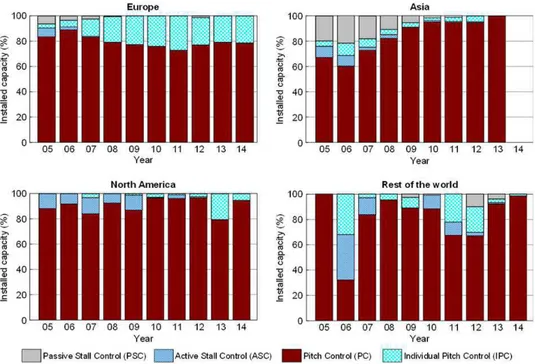
Figure 16 Wind turbine types according to drive train configuration [20] For the six drive train configurations described above, Figure 17 shows the market share for onshore HAWT installed during 2005-2014 [20]. According to JRC data, the share is not similar all over the world; indeed, the different price of raw materials in different continents making that some drive train configurations are more competitive than other. For example, the increasing price of the row material for permanent magnet generators in Europe and North America has been reflected on a reduction of a type D-PM drive train configuration [11]. Anyway, all over the world, it can be observed that type C configuration dominates the market with an increasing trends of types D, E and F while types A and B have recorded downward trends.

Figure 17 Evolution of the share of installed capacity by wind turbine configuration[20]. Source: JRC database

(47)

1.4.2.c Evolution of power control

The increasing penetrations of wind energy all over the world has raised a growing interest in their control with the purpose to extract more energy from wind, to reduce the mechanical loads and to reduce wind turbine damage and costs. Therefore, the quality of power control has a direct impact on the operation and maintenance costs of wind turbine, as discussed in [23].

In order to understand the approaches to control the extracted power in a HAWT a quick overview of the power conversion is presented.

Wind turbines work to convert the available power in the wind into shaft torque and then electrical energy. The available power in the wind, Pa [W], is define as:

7=1_{2 ‡ˆ‰}h (1)

where ‡ is the air density [Kg/m3_{], A is the swept area of the rotor [m}2_{] and v is the} wind speed [m/s].

Using the principles of conservation of momentum and energy, a complete conversion of available power can be achieved when the wind behind the wind turbine became stationary. However, since that the wind is the result of movement of air, a stationarity of wind behind the wind turbine can be reached only in no wind condition. Therefore, the wind turbine cannot extract all the energy from the wind. In 1919, Albert Betz proved that the maximum possible energy that can be extract cannot be more than 16/27, defined as Betz Limit, of the available power in the wind, Pa. However, no wind turbine has ever achieved that limit.

Actually, the energy extract from the wind turbines is define as:

2 = ŠI∗ 7= ŠI∗1_{2 ‡ˆ‰}h (2)

Where Cp is the power coefficient and it is a function of blade pitch β and the tip speed ratio λ (i.e. the ratio between the linear speed of the tip blade and incoming wind speed). Therefore, Cp is the only parameter that power controls can change to varying power of the wind turbines.

The operating region of a wind turbines and its power control are typically divided in four regions as shown in Figure 18 [25]:

• Region 1, for wind speed below the cut in, the generator is turned off; • Region 2, for wind speed between cut in and rated wind speed, the rotor

yaw is keep perpendicular to the wind direction and the blade pitch is set at the value that produces the maximum Cp (i.e. β*_{=0°). In this region, the} primary goal is to maximize the power available in the wind;