DISI - Via Sommarive, 5 - 38123 POVO, Trento - Italy
http://disi.unitn.it
JOINT LEARNING AND
OPTIMIZATION OF UNKNOWN
COMBINATORIAL UTILITY
FUNCTIONS
Paolo Campigotto, Andrea Passerini, Roberto
Battiti
March 2013
Joint learning and optimization of unknown combinatorial utility functions
Paolo Campigottoa, Andrea Passerinia, Roberto Battitia aDISI - Dipartimento di Ingegneria e Scienza dell’Informazione,
Universit`a degli Studi di Trento, Via Sommarive 14, I-38123 Povo, TN, Italy.
Abstract
This work considers the problem of automatically discovering the solution preferred by a decision maker (DM). Her preferences are formalized as a combinatorial utility function, but they are not fully defined at the beginning and need to be learnt during the search for the satisficing solution. The initial information is limited to a set of catalog features from which the decisional variables of the DM are to be selected.
An interactive optimization procedure is introduced, which iteratively learns an approximation of the utility func-tion modeling the quality of candidate solufunc-tions and uses it to generate novel candidates for the following refinement. The source of learning signals is the decision maker, who is fine-tuning her preferences based on the learning process triggered by the presentation of tentative solutions.
The proposed approach focuses on combinatorial utility functions consisting of a weighted sum of conjunctions of predicates in a certain theory of interest. The learning stage exploits the sparsity-inducing property of 1-norm regularization to learn a combinatorial function from the power set of all possible conjunctions of the predicates up to a certain degree. The optimization stage consists of maximizing the learnt combinatorial utility function to generate novel candidate solutions. The maximization is cast into an Optimization Modulo Theory problem, a recent formalism allowing to efficiently handle both discrete and continuous-valued decisional features. Experiments on realistic problems demonstrate the effectiveness of the method in focusing towards the optimal solution and its ability to recover from suboptimal initial choices.
Keywords:
Preference elicitation, machine learning, combinatorial optimization, Satisfiability, Satisfiability Modulo Theory, Optimization Modulo Theory.
1. Introduction
In real world optimization tasks, a significant portion of the problem-solving effort is usually devoted to specifying in a computable manner the function to be optimized. This modeling work consists of modifying and refining the problem definition on the basis of information elicited from the decision maker (DM). Typically, asking a user to quantify her real objectives a priori, without seeing any optimization results, is extremely difficult. Interactive decision making approaches handle this initial lack of complete knowledge by keeping the user in the loop of the optimization process. They use the information from the DM during the optimization task to guide the search towards the solution preferred by the user.
A paradigmatic case of incomplete problem definition is provided by multi-objective optimization problems, which consider the simultaneous optimal attainment of a set of conflicting objectives. While the DM usually can define the set of desirable objectives, she cannot define their relative importance, the trade-offs and the proper com-bination of them into an overall utility function. Several interactive multi-objective algorithms have been proposed to
Email addresses: [email protected] (Paolo Campigotto), [email protected] (Andrea Passerini), [email protected] (Roberto Battiti)
learn the utility function modeling the preferences of the DM, see e.g. [1] for a recent review and [2] for a recent ex-ample. They iteratively alternate preference elicitation (decision stage) and solution generation (optimization phase). At each iteration, the DM evaluates the proposed candidate solutions. The preference information obtained is used to refine a model of the DM preferences; new solutions are generated based on the learnt model. By adopting this approach, the DM preferences drive the search process and only a subset of the Pareto optimal solutions needs to be generated and evaluated.
In general, formalizing the user preferences into a mathematical model is not trivial: a model should capture the qualitative notion of preference and represent it as a quantitative function. Let us assume that the candidate solutions of the problem are described by a set of n features x1, . . . ,xn. The simplest and most used utility model is the additive
function, where the preference of the DM for the candidate solution x is given by the sum of sub-utility functions:
U(x) =
n X k=1
uk(xk)
with each sub-utility function ukis defined on a single feature xk. Additive utility models are appropriate under the assumption of preferential independence among the set of features [3]. Preferential independence exists when the DM preference for the values of a feature xidoes not depend on the fixed values of other features xj,j , i. Consider, for example, a costumer of a real estate company articulating her preferences by using only two attributes: the number of bedrooms (x1) and the distance from the city center (x2). Her preference over the values of x1is the same regardless
of the values of x2, and vice versa: she always prefers houses with two bedrooms over houses with one bedroom and
she always favors the location nearest to the city center.
Additive models fail to capture complex DM preferences including non-linear relationships among the features of the candidate solutions. For example, a customer willing to have a gym in the neighborhood in the case of candidate houses near the city center. When considering houses in the suburbs, the presence of free parking makes houses without a garage attractive (to keep price low) and, similarly, the proximity of green areas providing the opportunity for outdoor sport activities decreases her interest for a gym in the neighborhood. Generalized additive independence (GAI) [3] models overcome the limitation of simple additive models by encoding utilities as a sum of sub-utility “overlapping” functions: U(x) = p X k=1 uk(Xk) where Xk,k = 1 . . . p, are subsets of the n features that may be non-disjoint.
The papers [4, 5, 6] present a framework for the elicitation of GAI utilities based on the minimax regret decision criterion. The minimax regret criterion guarantees worst-case bounds on the quality of the decision made under uncertain knowledge of the DM preferences. In particular, the minimax regret optimal decision minimizes the worst case loss with respect to the possible realizations of the unknown DM utility function.
Recent work in the field of constraint programming [7] formalizes the user preferences in terms of soft constraints. In soft constraints, a generalization of hard constraints, each assignment to the variables of one constraint is associated with a preference value. A candidate solution to a set of soft constraints assigns a value to the variables of each constraint. The desirability of a candidate solution is computed by combining the preference values of its assignments to the variables of the different constraints. The work in [7] introduces an elicitation strategy for soft constraint problems with missing preferences, to find the solution preferred by the decision maker by asking the final user to reveal as few preferences as possible.
In this paper, soft constraints are cast into first-order logic formulas, with each formula being the conjunction of predicates in a certain theory of interest. The theory fixes the interpretation of the symbols used in the predicates (e.g., the theory of arithmetic for dealing with integer or real numbers). The DM preferences are represented by combina-torial utility functions which are weighted combinations of the first-order logic formulas. For example, consider the case of flight selection. The predicate x1+ x2 ≤ 5 hours defines the preference for a travel duration, calculated as
flight duration (x1) plus transfer time to the departure airport (x2), smaller than five hours. The predicate x3<2 states
the desirability for a flight with number of stopovers (x3) smaller than two. The weighted combination of the couple
of predicates articulates the DM preferences about the flight to book. Similarly to the GAI models, this representation of the DM preferences can express the combined effects of multiple non-linearly related decisional features. Our pref-erence elicitation algorithm formulates the combinatorial utility functions as Optimization Modulo Theory instances
where the objective function is unknown and has to be interactively learnt. Optimization Modulo Theory [8, 9] is an extension of Satisfiability Modulo Theory [10] (SMT), a powerful formalism to check the satisfiability of formulas in a decidable first-order theory. SMT has received increasing attention in recent years, thanks to a number of successful applications in areas like verification systems, planning and model checking. Optimization Modulo Theory extends SMT by considering optimization (MAX-SMT) problems. Rather than checking for the existence of a satisfying assignment as in SMT, the target is a satisfying assignment that minimizes a given cost function. The adoption of the Optimization Modulo Theory formalism enables a generic approach which efficiently handles both discrete and continuous-valued decisional features.
Our algorithm for the joint learning and optimization of the DM preferences consists of an iterative procedure alternating a search phase with a model refinement phase. At each step, the current approximation of the utility function is used to guide the search for optimal configurations; preference information is required for a subset of the recovered candidates, and the utility model is refined according to the feedback received. A set of randomly generated configurations is employed to initialize the utility model at the first iteration.
Unlike previous work on preference elicitation for constraint problems [7], our method does not assume to know in advance the decisional features of the user and their detailed combination. In the paper [7] soft constraint topology and structure is assumed to be known and the incomplete information consists of missing local preference values only. The initial amount of knowledge required by our approach is limited to a set of “catalog” features from which the decisional variables of the DM are selected. The limited initial knowledge translates in a sparse unknown utility function: only a fraction of the catalog features represent the decisional items of the DM and only a subset of the possible terms constructed from them defines the DM utility function. Furthermore, our method can handle uncertain, inconsistent and contradictory preference information from the final user, which characterizes many human decision processes. The robustness to noisy feedback from the DM distinguishes our approach also from the regret-based preference elicitation methods [4, 5, 6], where the bounds on the quality of the recommended solutions and the guarantee about the convergence to provably-optimal configurations are valid under the unrealistic assumption of noise-free and certain answers from the DM.
This paper introduces the first approach combining learning, interactive optimization and SMT. A preliminary version of our technique was presented in [11]. This manuscript considerably extends the preliminary version by a deeper comparison with the preference elicitation literature, a more detailed description of the Satisfiability Modulo Theory formalism and a wider experimental evaluation including also an additional benchmark designed in the spirit of real-world applications. Furthermore, the quantitative judgments asked to the DM in the preliminary version are replaced by less cognitive demanding queries, consisting of qualitative comparisons of candidate solutions.
The organization of the paper is as follows. Section 2 introduces our preference elicitation algorithm, while Sec-tion 3 analyzes its properties and its parameters setting. SecSec-tion 4 introduces SMT and OptimizaSec-tion Modulo Theory and explains how this formalism is used by our algorithm. Related work is discussed in Section 5. Experimental results in Section 6 on both synthetic and realistic problems demonstrate the effectiveness of our approach in focusing towards the optimal solutions, its robustness and its ability to recover from suboptimal initial choices. A discussion including potential research directions concludes the paper.
2. Overview of our approach
For ease of explanation, we first introduce the simplest formulation of our preference elicitation method, which considers Boolean decisional features only. The generalization to discrete and continuous-valued features is presented in Section 4. In the simplest formulation of our algorithm, candidate configurations are n dimensional vectors x consisting of Boolean catalog features. A priori knowledge of the problem is limited to the set of catalog features. The unknown combinatorial utility function expressing the DM preferences is the weighted combination of Boolean terms generated from the catalog features (weighted MAX-SAT instance), and it has to be jointly and interactively learned during the optimization process. Furthermore, the optimal utility function is complex enough to prevent exhaustive enumeration of possible solutions. The only assumption we make on the utility function is its sparsity, both in the number of features (from the whole set of catalog ones) and in the number of terms constructed from them. The assumption is grounded on the bounded rationality of a human DM, which can simultaneously handle only a limited number of features to make decisions, and drives some specific design choices of our optimization algorithm.
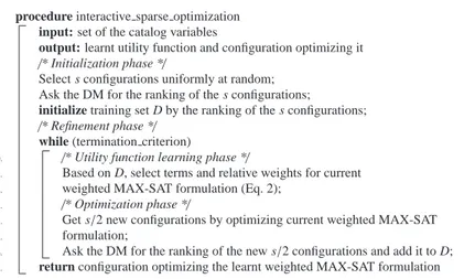
1. procedure interactive sparse optimization 2. input: set of the catalog variables
3. output: learnt utility function and configuration optimizing it 4. /* Initialization phase */
5. Select s configurations uniformly at random;
6. Ask the DM for the ranking of the s configurations;
7. initialize training set D by the ranking of the s configurations; 8. /* Refinement phase */
9. while (termination criterion)
10. /* Utility function learning phase */
11. Based on D, select terms and relative weights for current
12. weighted MAX-SAT formulation (Eq. 2);
13. /* Optimization phase */
14. Get s/2 new configurations by optimizing current weighted MAX-SAT
15. formulation;
16. Ask the DM for the ranking of the new s/2 configurations and add it to D;
17. return configuration optimizing the learnt weighted MAX-SAT formulation
Figure 1: Pseudocode for the interactive optimization algorithm. The parameter s defines the number of examples to be compared by the DM at the different iterations. The training set D contains the partial rankings of candidate solutions generated at the initialization phase and at the different iterations of the algorithm.
See Sections 3.5 and 7 for a discussion on how to generalize the approach to arbitrarily complex and dense utility functions, as could be found in optimizing machine rather than human decision processes.
Our method consists of an iterative procedure alternating a utility function learning phase with a search phase. At each step, the current approximation of the utility function, represented as a weighted MAX-SAT instance, is used to guide the search for optimal configurations. A subset of candidate configurations is obtained by solving the weighted MAX-SAT instance (search phase). Preference information is required for these candidates, and the utility model is refined according to the feedback received (learning phase). In particular, the DM expresses her preferences by ranking the candidate solutions generated at each iteration of our method. Thus the preference information collected at the n-th iteration consists of the partial rankings generated at the iteration 1, 2, . . . , n − 1. A set of randomly generated configurations to be ranked is employed to initialize the utility model. The pseudocode of our algorithm is in Fig. 1. The initialization, learning and search phases of our approach are detailed below, while its properties and the parameters setting are discussed in Sec. 3.
2.1. Initializing the algorithm
A set of random configurations is generated to approximate the DM utility function at the first iteration. Each Boolean feature is assigned a truth value independently and uniformly at random. The evaluation of diverse examples stimulates the preference expression, especially when the user is still uncertain about her final preference [12]. In particular, the diversity of the examples helps the user to reveal the hidden preferences: in many cases the decision maker is not aware of all preferences until she sees them violated. For example, a user does not usually think about the preference for an intermediate airport until one solution suggests an airplane change in a place she dislikes [12].
2.2. Learning an approximation of the utility function
The refinement of the utility model consists of learning the weights of the terms, discarding the terms with zero weight. It includes both the selection of the relevant features from the catalog set and the learning of their detailed combination from the space of all possible conjunction up to certain degree d. To identify sparse solutions, chara-terized by few terms with non-zero weights, we adopt 1-norm regularization, which provides an embedded feature selection capability [13]. Features selection is crucial to maximize the learning accuracy with data sets characterized by redundant and irrelevant features [14]. The “Least absolute shrinkage and selection operator” (Lasso) [13] is a pop-ular method for regression tasks which uses 1-norm regpop-ularization to achieve a sparse solution. Let D = (xi,yi)i=1...m be the set of m training examples, where xicontains the feature values of the i-th example and yirepresents its score
value. The loss+penalty formulation of Lasso regression is defined by the following optimization problem: min w∈IR m X i=1 (yi−wT · Φ(xi))2+ λ||w||1 (1)
where w is the weight vector and the mapping function Φ projects the input vector to a higher dimensional space. The square loss functionPmi=1(yi−wT· Φ(xi))2measures the empirical risk as the sum of the squared training errors.
The penalty function consists of 1-norm regularization, favouring automated feature selection. The regularization parameter λ trade-offs the penalty and loss terms.
In our context, the mapping function Φ projects sample vectors to the space of all possible conjunctions up to d Boolean variables. The score value yirepresents the quantitative evaluation of the decision maker for the solution xi. The preference scores are taken from a predefined ordered set expressing the desirability levels for the candidate solutions. This was the approach adopted in our original formulation [11]. However, comparing solutions is a much more affordable task for the DM than assigning preference scores. We thus cast the task of learning the utility function into a ranking problem.
Given a set of m candidate solutions (x1, . . . ,xm) and an order relation ≻ such that xi ≻ xj if xi should be preferred to xj, a ranking (y1, . . . ,ym) of the m solutions can be specified as a permutation of the first m natural numbers such that yi < yj if xi ≻ xj. Learning to rank consists of learning a ranking function r from a dataset D = {(x(i)1, . . . ,x(i)mi), (y (i) 1, . . . ,y (i) mi)} s
i=1, made of s sets with their desired rankings. The ranking function r associates each candidate instance with a real number, with the aim that r(xi) > r(xj) ⇐⇒ xi ≻xj. In this way, it provides an ordering that agrees with the observed training examples. Given the ranking dataset D, the 1-norm regularization formulation can be adapted to learn the ranking function r by imposing constraints on the correct pairwise ordering of solutions within a set: r(x(i)h) > r(x(i)k) ⇐⇒ yh(i) <y(i)k . In the case of support vector machines, r(x) = wT· Φ(x) and r(xi) > r(xj) ⇐⇒ wT ·(Φ(xi) − Φ(xj)) > 0. The resulting loss+penalty formulation for 1-norm support vector machine can be written as:
min w∈IR s X i=1 X h,k,y(i)h<y(i)k
[1 − wT·(Φ(x(i)h) − Φ(x(i)k))]++ λ||w||1 (2)
where subscript “+” indicates the positive part. The first term is the so-called empirical Hinge Loss, adapted for ranking tasks. It assigns a linear penalty to inconsistencies in the ranking, i.e., cases where a less preferred solution is ranked higher than a more preferred one, or correct rankings where the score difference is smaller than the support vector machine margin, i.e., 0 < wT ·(Φ(x(i)
h ) − Φ(x
(i)
k )) < 1. The formulation in Eq. (2) handles ties and partial rankings, as constraints are only included whenever two examples should be ranked differently.
The learnt function ˆf (x) = wT· Φ(x), where w is the solution of the ranking problem, will be used as the novel approximation of the utility function f of the DM.
2.3. Optimizing the learnt utility function
The learnt utility function ˆf expressing the approximation of the DM preferences is represented as a weighted
MAX-SAT instance. The set of novel candidate solutions to be ranked by the DM is obtained by applying a complete solver over the weighted MAX-SAT instance. The size of the weighted MAX-SAT instance is indeed bounded by the limited cognitive capabilities of the human DM. The adoption of local search techniques for large scale problems will be discussed in Sec. 7. The MAX-SAT solver returns an optimizer for the input problem, i.e., the configuration x∗ maximizing the weighted sum of the terms representing ˆf . However, the currently learnt utility ˆf is only an approximation of the true unknown DM utility. In order to refine this approximation, a diversified set of informative training examples is needed. In our algorithm, the creation of informative training examples (active learning) is driven by the following principles:
1. the generation of top-quality configurations, consistent with the learnt DM preferences;
2. the generation of diversified configurations, i.e., alternative possibly suboptimal configurations with respect to the learnt utility ˆf ;
3. the search for the DM features which were not recovered by the current approximation ˆf , i.e., features not
appearing in any of the terms in ˆf .
The rationale for the first principle is the modeling of the relevant areas of the fitness surface (i.e., the shape of the utility function locally guiding the search to the correct direction) and the search for solutions satisficing the DM. As a matter of fact, a preference elicitation system that asks to rank low quality configurations will be likely considered useless or annoying by the user [15]. The second principle favours the exploration of the relationships among the features recovered by the current preference model ˆf . Finally, as the learnt formulation of ˆf may miss some of the
DM decisional features, their search is promoted by the third principle. Let us note that the need for a set of good, given the current known preferences, and diverse configurations to be evaluated by the user is pointed out, e.g., in [12]. Based on the above principles, our active learning strategy works as follows. In order to obtain multiple solutions in addition to x∗, the MAX-SAT formulation of ˆf is modified by including the hard constraint generated by the
disjunction of all the terms of ˆf unsatisfied by x∗. Unlike the weighted terms, which may or may not be satisfied, hard constraints do not have a weight value and have to be satisfied. For example, let t1and t5be the terms of ˆf unsatisfied
by x∗, then the hard constraint becomes:
(t1∨t5) (3)
If the term tiis associated with a weight wi <0, it is satisfied when its value is false. Therefore, if, e.g., the weight
w1is negative, the hard constraint in Eq. (3) becomes (¬t1∨t5). If x∗satisfies all the terms of ˆf , i.e., ˆf (x∗) = 0, the
additional hard constraint generated is:
(¬x∗1∨ ¬x∗2. . . ∨ ¬x∗n)
which excludes x∗from the set of feasible solutions. The inclusion of the hard constraints is motivated by the second principle, as the satisfaction of at least one of the terms unsatisfied by x∗is usually obtained by configurations differing in more than a single Boolean value from x∗. The modified formulation of ˆf is then optimized (first principle) to obtain the the second candidate solution x∗∗. The catalog features not included in the formulation of ˆf are set uniformly at random in x∗∗(third principle). Let us note that if these features are truly irrelevant for the DM, setting them at random should not affect the evaluation of the candidate solutions. If on the other hand some of them are needed to explain the DM preferences, driving their elicitation can allow to identify the deficiencies of the current approximation ˆf and
recover previously discarded relevant features.
The process is repeated, progressively adding hard constraints for each of the previously generated solutions, until the desired number of configurations have been generated or the hard constraints made the MAX-SAT instance unsat-isfiable. Finally, the DM will rank the new candidate solutions based on her preferences and the ranking information will be included in the training examples set D for the following refinements of ˆf .
3. Analysis of our approach
The number of refinement iterations does not need to be fixed at the beginning. The DM may ask for an additional iteration by comparing the recovered candidates with her own preferences. The termination criterion is thus repre-sented by the satisfaction of the DM with the prerepre-sented candidate solutions. Furthermore, the number of candidates to be evaluated at each iteration is arbitrary. In the settings used here, we use s configurations at the first iteration and s/2 examples at each following iteration. A larger number of configurations is suggested at the first iteration to stimulate the preference expression of the DM, as discussed in Sec. 2.1, and to generate a good initial model. The following iterations generate solutions distributed in the promising regions of the search space. The goal of our ap-proach is indeed the identification of the solution preferred by the user (learning to optimize) rather than an accurate global approximation of the DM utility function (learning per se). This requires a shift of paradigm with respect to standard machine learning strategies, in order to model the relevant areas of the optimization fitness surface rather than reconstruct it entirely.
3.1. Convergence of the algorithm
The limited size of the MAX-SAT instances (or MAX-SMT, as it will be explained in Sec. 4) enables the systematic investigation of the search space by means of a complete solver (the adoption of local search for larger instances is discussed in Sec. 7), which ensures the identification of the solution x∗ maximizing the learnt utility model ˆf
(completeness property). However, our algorithm cannot guarantee the quality of the model ˆf approximating the true
DM utilities, and therefore the optimality of x∗(or bounds on its quality) w.r.t. the true DM utilities cannot be proved. As a matter of fact, the learning task in Eq. (2) is convex, and thus guaranteed to converge to its global optimum, but the consistency of the learning algorithm with the true underlying user utility is only guaranteed asymptotically (i.e., provided that enough training data is available). On the other hand, our algorithm does not need to learn the exact form of the DM utility function. The goal of our approach is indeed to elicit as few preference information from the DM as possible in order to identify her favourite solution (learning to optimize). For example, consider the toy DM utility function represented by the negation of a single ternary term: ¬(x1∧x2∧x3). The approximation of the DM
utility function consisting, e.g., of the formula ¬x1 is sufficient to find the favourite DM solution. More in general,
only the shape of the utility function locally guiding the search to the correct direction is actually needed. Indeed the experimental results reported in Sec. 6 show the ability of our method in identifying the optimal solution and the improvements in the quality of the candidate solutions when increasing the number of refinement iterations (anytime property).
3.2. User cognitive load
In preference elicitation systems the acquisition of feedback from a human DM, characterized by limited patience and bounded rationality, is a crucial issue. Although providing explicit weights and mathematical formulas is in general prohibitive for the DM, she can definitely evaluate the returned solutions. In the preliminary version of our algorithm [11] quantitative judgments are asked to the DM. However, asking the final user for precise scores is in many cases inappropriate or even impossible. Most of the users are typically more confident in comparing solutions, providing qualitative judgments like “I prefer solution x′to solution x′′”, rather than in specifying how much they prefer x′over x′′. In order to reduce the embarrassment of the decision maker when specifying precise preference scores, in this paper the evaluation by the user consists of just comparing and ranking candidate solutions.
3.3. Robustness to inaccurate preference information
Assuming that the user provides accurate and consistent preference information at any time is not realistic, due to the bounded rationality and the limited capabilities of the humans when making decisions. Different factors may generate uncertain and inconsistent feedback from the DM, including occasional inattentions, embarrassment when comparing very similar solutions or solutions which are very different from her favourite one, DM fatigue increasing with the number of queries answered. The adoption of regularized machine learning strategies in our algorithm enables a robust approach that can handle ties and inaccurate rankings from the DM.
3.4. Computational complexity
The cognitive capabilities of the humans when making decisions limit the number n of catalog features and the size d of the Boolean terms. Therefore, the learning phase (problem (2)) is accomplished in a negligible amount of time (w.r.t. the user response time). Analogous observation holds for the computational effort required by the search phase. Proposing a query consists of generating c candidates to be ranked. Each candidate is obtained by a run of the complete MAX-SAT solver. Even if the search space size is 2n, the bounded value of n and the efficient performance of modern SAT solvers, that can manage problems with thousands of variables and millions of clauses, enable the completion of the search phase in a negligible amount of time. An efficient implementation of the search phase is also achieved in the more general case represented by MAX-SMT instances, that will be discussed in Sec. 4, as the state-of-the-art SMT solvers are built on top of modern SAT solvers. Finally, the estimation of the cognitive load of the DM is O(c log c), with c being the number of candidates to be ranked. In the experiments reported in Sec. 6, the value of c used in the refinement phase varies from 5 to 50. Keeping c low limits the computational effort of the DM. As a matter of fact, the DM typically prefers to rank small batches of good quality solutions rather than a single large batch of candidates, including also lower quality ones. Furthermore, the chance of obtaining inaccurate feedback from the DM increases when she evaluates solutions which are very different from her favourite one. Therefore, a rule of thumb for the algorithm configuration consists of keeping the value of c low and increasing the number of refinement iterations.
3.5. Scalability of the algorithm
The adoption of 1-norm regularization for the formulation of the learning problem requires that the input catalog features are explicitly projected in the space of all possible Boolean terms which can be generated by their combina-tion. Dealing with the explicit projection Φ in Eq. (2) is tractable only for a rather limited number of catalog features and size of conjunctions d. However, this will typically be the case when interacting with a human DM. The bounded rationality of humans indeed allows them to handle non-linear interactions just among a small number of features.
A possible alternative formulation consists of directly learning a non-linear function of the features, without explic-itly projecting them to the resulting higher dimensional space. This can be achieved by replacing 1-norm regularization with 2-norm in Eq. (2), thus recovering the original support vector ranking formulation [16, 17], and considering the kernelized version of the resulting dual problem. A similar solution for the regression (rather than ranking) formula-tion and plain MAX-SAT problems (rather than MAX-SMT, see later) was considered in our previous work [11]. As expected, the experimental results showed the superior performance of 1-norm over 2-norm regularization in a setting with many irrelevant noisy features, due to its sparsity-inducing property. See Section 7 for a discussion on how to adapt the full MAX-SMT preference learning formulation to deal with implicit feature spaces.
4. Satisfiability Modulo Theory
In the previous section, we assumed our optimization task could be cast into a propositional Satisfiability problem. However, the formalism of plain propositional logic is not suitable or expressive enough to represent many real-world applications, arising, for example, in the fields of real-time control system design and formal software verification. For example, software verification applications need reasoning about equalities, arithmetic operations and data struc-tures. These problems require or are more naturally described in more expressive theories as first-order logic (FOL), involving quantifiers, functions and predicates. Consider the toy example represented by the following formula from the theory of arithmetic over integers:
x + y + z ≤ 4, x, y, z ∈ {1, 2, 3}
We are interested in deciding whether there is an assignment of integer values to the variables x, y and z satisfying the formula. A possible encoding into an equisatisfiable SAT proposition is given by:
(x1∧y1∧z1) ∨ (x1∧y1∧z2) ∨ (x1∧y2∧z1) ∨ . . .
where xi, yi, zi, with i = 1, 2, 3, is a Boolean variable which is true when the integer-valued variable x, y, z is assigned the value i, respectively. Let us note the blow-up in the translation affecting the SAT instance size. In general, propositional logic is not expressive enough for the efficient encoding of many real world tasks: important structural information may be lost or exponential blow-up in the formula size may be caused (e.g., up to a 232factor to represent
all the candidate values that a 32-bit integer variable may assume).
Satisfiability Modulo Theory (SMT) [10, 18] problems generalize SAT problems by considering the satisfiability
of a FOL formula with respect to a certain background theory T fixing the interpretation of (some of the) predicate and function symbols. Any procedure designed to solve a SMT problem is called SMT solver. Popular examples of useful theories include various theories of arithmetic over reals or integers such as linear or difference ones. Linear arithmetic considers + and − functions alone, applied to either numerical constants or variables, plus multiplication by a numerical constant. Difference arithmetic is a fragment of linear arithmetic limiting legal predicates to the form
x − y ≤ c, where x, y are variables and c is a numerical constant. A number of theories have been studied apart from
standard arithmetic ones. Machine arithmetic, for instance, is more naturally modeled by the theory of bit-vector arithmetic, which includes bit-wise operations. Other theories exist for data structures such as lists and strings [10].
Different approaches have been developed to solve SMT problems. When deciding the satisfiability of a first-order formula ϕ in a given theory T , a general purpose FOL reasoning system such as Prolog, based on the resolution calculus, needs to add to the formula a conjunction of all the axioms in T . This is, e.g., the standard setting in inductive logic programming when verifying whether a certain hypothesis covers an example given the available background knowledge. Let us note that, whenever the cost of including such additional background theory is affordable, our optimization algorithm can be applied rather straightforwardly. Unfortunately, adding all axioms of T is not viable for many theories of interest: consider for instance the theory of arithmetic, which defines the interpretation of symbols such as +, ≥, 0, 5.
An alternative approach is represented by eager SMT solvers. They translate the original formula ϕ taken from the input theory T into an equisatisfiable propositional formula in one single step. In this way, any off-the-shelf SAT solver can be used to check the satisfiability of the generated propositional formula. The SAT solver is called once. However, a specific translator has to be developed for each theory of interest. Furthermore, the translation of
all the theory-specific information is required at the beginning of the search process (hence the name “eager”), likely
resulting in large SAT formulas. Although optimizations in the translation are possible, there is a trade-off between the degree of optimization and the time required by the SAT encoding. Let us note the analogy with compilers, optimizing the low-level object code (the SAT formula in our context) generated from a high-level program (the SMT problem formulation) [10].
A more efficient approach is based on incremental translations and calls to the SAT solver. This is the case of lazy SMT solvers, where the theory-specific information is incrementally encoded in the SAT formulation of the problem. In particular, the lazy approach exploits specialized reasoning methods for the background theory of interest. When integrated as submodules in a SMT solver, these theory-specific reasoning methods are often referred as solvers. T-solvers are efficient decision procedures typically developed to check the satisfiability of conjunctions of literals (i.e., atomic formulas and their negations) over the given theory T . The generalization to arbitrary propositional structures is handled in conjunction with the SAT solver integrated in the SMT solver.
In this work we focus on lazy SMT solvers and their optimization variant, which we integrated in our optimization algorithm. The rest of this section provides details about lazy SMT solvers search process and introduces Optimization Modulo Theory (OMT) solvers handling weighted Maximum Satisfiability Modulo Theory (MAX-SMT) problems. Finally, the integration of MAX-SMT solvers in our optimization approach is discussed.
4.1. Lazy Satisfiability Modulo Theory solvers
The search process of a lazy SMT solver alternates calls to the Satisfiability and the theory solver respectively, until a solution satisfying both solvers is retrieved or the problem is found to be unsatisfiable. Let ϕ be a formula in a certain theory T , made of a set of n predicates A = {a1, . . . ,an}. A mapping α maps ϕ into a propositional formula α(ϕ) by replacing its predicates with propositional variables pi= α(ai). The inverse mapping β replaces propositional variables with their corresponding predicates, i.e., β(pi) = ai. For example, consider the following formula in the arithmetic theory over integers:
x + y + z ≤ 3 ∧ (x ≤ y ∨ z = 2) ∧ (x ≥ 2 ∨ x , z) (4) where x, y, z are integer-valued variables. Then, p1 = α(x + y + z ≤ 3), p2 = α(x ≤ y), p3 = α(z = 2), p4 = α(x ≥ 2)
and p5= α(x , z). The resulting propositional formula α(ϕ) is:
p1∧(p2∨p3) ∧ (p4∨p5)
Let us note that the truth assignment
p1= ⊤, p2= ⊥, p3= ⊤, p4= ⊤, p5= ⊥
where ⊤, ⊥ symbols encode true and false truth values, respectively, is equivalent to the statement
x + y + z ≤ 3 ∧ x > y ∧ z = 2 ∧ x ≥ 2 ∧ x = z
in the theory T.
The SAT solver integrated in the SMT solver searches a solution of the propositional formula α(ϕ). If the proposi-tional formula in unsatisfiable, the original formula ϕ is also unsatisfiable and the whole SMT solver stops. Otherwise, the SAT solver provides a truth assignment satisfying α(ϕ). Considering the above example, it may be:
p1= ⊤, p2= ⊤, p3= ⊤, p4= ⊤, p5= ⊤ (5)
The T-sover is used to validate the assignment (i.e., the conjunction of truth values) produced by the SAT solver. The predicates are evaluated using the rules of the theory T . If the validation is successful, the SMT solver stops returning the assignment of values to the variables in T satisfying ϕ. Otherwise, when the T -solver detects unsatisfiability, an
1. procedure SMT solver(ϕ) 2. ψ = α(ϕ)
3. while (true)
4. (r,M) ← SAT(ψ)
5. if r = unsat then return unsat
6. (r,J) ← T-Solver(β(M))
7. if r = sat then return sat
8. C ←Wl∈J¬α(l)
9. ψ ← ψ ∧C
Figure 2: Pseudocode for a basic lazy SMT solver.
additional constraint explaining (i.e, justifying) the unsatisfiability is included in α(ϕ) and the SAT solver is asked for a new assignment. For example, the assignment in Eq. 5 is not valid in the arithmetic theory over integers. Applying the inverse mapping β, we obtain:
x + y + z ≤ 3 ∧ x ≤ y ∧ z = 2 ∧ x ≥ 2 ∧ x , z
which is unsatisfiable as z is set to the value two while x and y must be larger than value two. A possible justification explaining the unsatisfiability is given by the following constraint:
¬(p1∧p2∧p3∧p4)
which will be included in the propositional formula α(ϕ) for the following calls to the SAT solver. Continuing with the toy example, assume that the second call to the SAT solver returns the following truth assignment:
p1= ⊤, p2= ⊥, p3= ⊤, p4= ⊥, p5= ⊤ (6)
satisfying the above justification. Restoring the interpretation of the propositional variables pi, we obtain:
x + y + z ≤ 3 ∧ x > y ∧ z = 2 ∧ x < 2 ∧ x , z
which is satisfied by posing, e.g., x = 1, y = 0, z = 2.
The term lazy denoting this approach is due to the incremental strategy generating constraints on demand. On the contrary, eager methods produce all the constraints in one single step before the execution of the SAT solver.
Figure 2 reports the basic form [18] of a SMT algorithm.SAT(ψ) calls the SAT solver on the ψ instance, returning a pair (r, M), where r issat if the instance is satisfiable, unsat otherwise. In the former case, M is a truth assignment satisfying ψ. T-Solver(S) calls the theory solver on the formula S and returns a pair (r, J), where r indicates if the formula is satisfiable. If r =unsat, J is a justification for S , i.e., any unsatisfiable subset J ⊂ S . The next iteration calls the SAT solver on an extended instance accounting for this justification.
Off-the-shelf solvers introduce a number of refinements to this basic strategy, by pursuing a tighter integration between the SAT and the theory solvers. A common approach consists of pruning the search space for the SAT solver by calling the theory solver on partial assignments and propagating its results. Finally, combination methods exist to jointly employ different theories, see [19] for a basic procedure.
4.2. Weighted MAX-SMT and Optimization Modulo Theory solvers
Weighted MAX-SMT generalizes SMT problem much like weighted MAX-SAT does with SAT ones. Given a cost function c, an assignment s in the input theory T is sought with minimum c(s). The simplest formulation for the MAX-SMT problem consists of assigning a weight to each part (i.e., constraint) of the Boolean formula to be jointly satisfied. Weights represent penalties or costs for violating the constraints and are expressed by positive natural or real numbers. The cost function c(s) is defined by the sum of the weights of the constraints unsatisfied under the assignment s.
While a body of works exist addressing weighted MAX-SAT problems, MAX-SMT task has been tackled only recently [8, 9, 20] and very few solvers have been developed. In particular, optimization in SMT was first introduced
by the work in [8]. Let {(C1,w1), . . . , (Cm,wm)} the set of the weighted constraints, where Ciand wiidentify the i-th
constraint and its associated weight, respectively. Clearly, the cost function c takes values from the interval [0, W], with W = w1+ . . . + wm. A simple effective method [8] to obtain solutions with cost c(s) at most ¯W, with ¯W < W, consists of generating m additional constraints (Ci∨pi) , i = 1 . . . m, with pia fresh propositional variable. The initial background theory T is augmented with the integers and with the following assertions:
pi→(ki= wi), i = 1 . . . m
¬pi→(ki= 0), i = 1 . . . m
k1+ . . . + km≤ ¯W
In this way, any assignment s with cost larger than the upper bound ¯W on the cost function is inconsistent with the
augmented input theory. The search for the optimal assignment s∗is based on a branch and bound technique. Each time a lower upper bound ¯W′ < ¯W on the cost function is computed, the theory is updated by replacing ¯W with ¯W′ (this operation is called “theory strengthening”). A sequence of theories with an increasingly tight upper bound on the cost function is therefore generated. This strategy is referred to as “SMT with progressively stronger theories”. A different approach to handle MAX-SMT is used in the paper [9], where a theory of costs C is introduced to handle cost functions in SMT and a specialized theory-solver for C is developed within the standard lazy SMT schema.
4.3. Preference elicitation with the MAX-SMT formalism
The adoption of the MAX-SMT formalism in our approach enables an efficient representation of non-Boolean decisional features. The framework introduced in Sec. 2 does not need to be changed in the case of non-Boolean decisional features, because the effort required to handle non-Boolean encodings is completely performed by the MAX-SMT solver. As a matter of fact, when representing user preferences in the SMT setting, the DM utility function f is expressed as a weighted sum of terms, where a term is the conjunction of up to d predicates defined over the variables in the theory T . The set of all possible predicates represents the search space S of the MAX-SAT solver integrated in the MAX-SMT solver. Our approach learns an approximation ˆf of f and gets one of its
optimizers from the MAX-SMT solver, as an assignment to the decision variables in the input theory T involved in the predicates of ˆf . The decision variables in T that are not used in the current formulation ˆf are assigned values
selected independently and uniformly at random from the their domains. In this way, a complete assignment to the variables in the input theory (i.e., a candidate solution in T ) is obtained. The candidate solution in turn determines an assignment p∗= (p∗
1, . . . ,p ∗
n) of Boolean values (p∗i = {true, false}) to the predicates in S .
The diversification strategy to obtain multiple candidates solutions is the same as described in Sec. 2.3. The sequential optimization of ˆf is performed, with the additional hard constraint generated by the disjunction of all the
terms of ˆf unsatisfied by p∗. If p∗satisfies all the terms of ˆf , the additional hard constraint consists of:
(¬p∗1∨ ¬p∗2. . . ∨ ¬p∗n) which excludes p∗from the feasible solutions set of ˆf .
5. Related work
The problem of automatically learning utility functions and eliciting preferences from users is widely studied within the Artificial Intelligence community [21]. A popular approach to model the uncertain knowledge about the DM preferences consists of assuming a set of hypotheses, with no belief on the strength of the hypotheses. The set of hypotheses contains the feasible utility functions and reflects the partial knowledge about the DM preferences. The uncertainty about the DM preferences is decreased by restricting the feasible hypothesis set, when relevant preference information is received during the elicitation process. This approach is often referred to as reasoning under strict uncertainty [22]. An alternative uncertainty model consists of defining a probability distribution over the hypotheses. This is the case of Bayesian approaches to preference elicitation [23, 15, 24, 25].
Our work casts the preference elicitation task into the problem of learning combinatorial optimization instances to be optimized for the generation of additional candidate solutions. The learning phase is accomplished by applying techniques from Machine Learning, while the optimization (or search) stage is based on Combinatorial Optimization
methods. Our approach satisfies the main principles [15] needed for practical applicability of preference elicitation techniques: the need for multi-attribute models, i.e., candidate configurations represented by means of multiple de-cisional features or attributes; the quest for real-time interaction with the DM, where both the query generation and the solutions recommendation must be accomplished in no more than few seconds; the robustness to inconsistent and contradictory feedback from the DM; the need for cognitively affordable queries to the user, i.e., comparison queries; the demand for scalable methods, that evaluate at each preference elicitation stage a number of candidate queries that grows linearly in the cardinality of the solutions space.
From the perspective of Machine Learning/Artificial Intelligence, the closest approaches to ours are the methods based on the minimax regret criterion [4, 5, 6], while a recent technique [7] developed within the Constraint Program-ming community shares with our algorithm the combinatorial formulation of the DM preferences. In the following, we review these alternative approaches and compare them with our technique.
5.1. Minimax regret-based approaches
The methods developed in the papers [4, 5, 6] perform preference elicitation under strict uncertainty. They assume a parametric formulation of the candidate utility function (hypothesis) in the feasible utility set U. The parametriza-tion, based on the generalized additive independence models discussed in Sec. 1, enables a compact way to specify the feasible set, which is represented by bounds and constrains on the parameters. Uncertainty is thus reduced by tightening the constraints or increasing (decreasing) the lower (upper) bounds.
To make decisions with the partial utility information under strict uncertainty and, in particular, to select the final configuration to be returned to the DM, the minimax regret decision criterion is used. It prescribes the configuration that minimizes the maximum regret with respect to all the possible realizations of the DM utility function in the set U. Thus, the minimax regret criterion minimizes the worst-case loss with respect to the possible realizations of the DM utility function. In detail, the minimax regret criterion is defined in two stages, building on the maximum pairwise regret and the maximum regret. The maximum pairwise regret of configuration x with respect to configuration x′over the feasible utility set U is defined as:
R(x, x′,U) = max
u∈U u(x
′) − u(x) (7)
This formulation can be interpreted by assuming an adversary that can impose any DM utility function u in U and chooses the one that maximizes the regret of selecting solution x. The function uw= argmax R(x, x′,U) is thus termed the “adversary’s utility” or “witness utility”. The maximum regret of choosing solution x with respect to the feasible utility set U is defined as:
MR(x, U) = max
x′ R(x, x
′,U) (8)
Within the “adversary metaphor”, let us note that the x′ chosen by the adversary for the specific uwis the optimal decision under uw (i.e., x′ maximizes uw) and any alternative choice would give the adversary less utility and thus reduce the user regret. Finally, the minimax regret of the feasible utility set U is as follows:
MMR(U) = min
x MR(x, U) (9)
and the solution xr= argmin MR(x, U) minimizing the maximum regret is the configuration recommended to the DM by the minimax regret decision criterion. The quality of the solution xr is guaranteed to be no more than MMR(U) away from the quality of the DM favourite solution, and no alternative solution has a better guarantee, i.e., for all x , xr, MR(x, U) ≥ MMR(U).
The initial bounds about the utility parameters defined by the DM are not usually tight enough to identify config-urations with provably low regret, and a configuration satisficing the DM cannot be recommended without eliciting additional preference information. This is achieved through an interactive elicitation algorithm that asks queries to the DM and, based on the information elicited, refines the bounds and the constraints on the utility parameters. The generic framework of the approach is as follows:
input: initial constraints (e.g., bounds) on the utility parameters defining
the initial feasible set U compute minimax regret MMR(U);
repeat until termination criterion
ask query q;
refine U by updating the constraints over utility parameters to reflect the response to q;
recompute MMR(U) with respect to the refined set U;
return to the DM the solution xrminimizing MR(x, U)
Computationally tractable techniques have been proposed [4, 5, 6] to compute the minimax regret MMR (U). The iterative algorithm may be stopped by the DM when she is satisfied by the returned solution xror when the minimax regret MMR(U) reaches a certain level τ. When the minimax regret is reduced to the value zero, the solution xr returned by the algorithm is guaranteed to be the DM favourite solution. The minimax regret-based approach also enables a principled method to define informative queries that will be asked the DM (query optimization), and different query strategies have been proposed [4, 5, 6].
5.1.1. Comparison with our method
While the target of our work is a preference elicitation method approximately correct with high probability, the minimax regret-based approaches assume an adversarial entity that acts to maximize the DM regret and they aim at beating the adversary by recommending the best solution with respect to the worst case loss. However, this adversarial model is not always strongly motivated by real-world applications, where users are typically interested in the actual obtained results rather than in regret. The main advantage of the regret-based approaches with respect to our algorithm is the ability to provide a lower bound about the quality of the recommended solution and guarantee the convergence to provably-optimal results. However, these theoretical guarantees are valid under the assumption that the feasible set U contains the true DM utility function at any iteration of the elicitation process. That is, the regret-based meth-ods do not consider the uncertain and inconsistent preference information characterizing the typical human decision processes. As a matter of fact, uncertain feedback from the DM translates into constraints on the utility parameters that can potentially rule out the true utility from the feasible set U. Furthermore, the best performance observed in the experiments presented in the paper [4] is achieved by query strategies that include standard gamble queries, which require the users to state their preference over a probability distribution of configurations. These queries demand a higher DM cognitive load than the comparison queries adopted in our work, and thus in real-world applications they are more prone to errors and inconsistent answers from the users. Without suitable modifications (e.g., constraints relaxation) to recover from the inevitable uncertain and inconsistent preference information elicited from the DM, regret-based approaches cannot be applied in the realistic problem settings and the noisy test cases that we consider in this work.
5.2. Preference elicitation methods based on constraint satisfaction
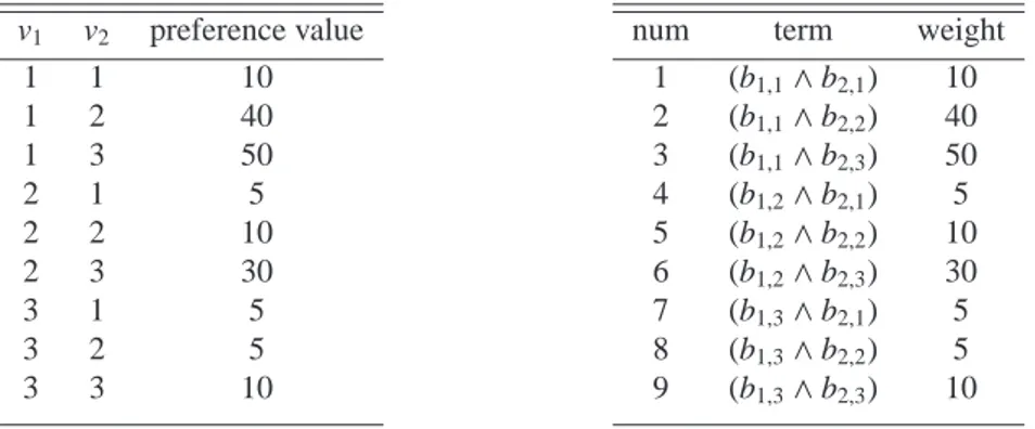
Recent work in the field of constraint programming [7] shares with our technique the combinatorial approach to model user preferences. It defines the user preferences in terms of soft constraints and introduces constraint opti-mization problems where the DM preferences are not completely known before the solving process starts. Let us first briefly describe the c-semiring formalism [26] adopted in paper [7] to model soft constraints.
In soft constraints, a generalization of hard constraints, each assignment to the variables of one constraint is associated with a preference value taken from a preference set. The preference value represents the level of desirability of the assignment to the variables of the constraint. As the preference score is associated to a partial assignment to the problem variables, it represents a local preference value. The desirability of a complete assignment is defined by a global preference score, computed by applying a combination operator to the local preference values. A set of soft constraints generates an order (partial or total) over the complete assignments of the variables of the problem. Given two solutions of the problem, the preferred one is selected by computing their global preference levels. Soft constraints are represented by an algebraic structure, called c-semiring (where letter “c” stays for “constraint”), providing two operations for combining (×) and comparing (+) preference values. In detail, the c-semiring is a tuple (A, +, ×, 0, 1) where:
• A is a set and 0, 1 ∈ A;
• ×is commutative, associative, distributes over +; 1 is its unit element and 0 is its absorbing element.
Let us note that a c-semiring is a semiring with additional properties for the two operations: the operation + must be idempotent and with 1 as absorbing element, the operation × must be commutative. The relation ≤A over A,
a2 ≤A a1iff a2+ a1 = a1, is a partial order, with 0 and 1 its minimum and maximum elements, respectively. The
relation ≤A allows to compare (some of) the desirability levels, with a2 ≤A a1 meaning that a1 is “better” than a2; 0
and 1 represent the worst and the best preference levels, respectively, and the operations + and × are monotone on ≤A. Consider, e.g., the following instance of c-semiring:
({5, 10, 15, . . . , 50}, max, min, 5, 50)
with preference values from the set {5, 10, 15, . . . , 50} and elements 0 and 1 represented by the values 5 and 50, respectively. The desirability of a complete assignment is obtained by taking its minimum local preference value. A complete assignment c1with preference score a1is preferred to a complete assignment c2with lower preference score a2. That is, a2≤Aa1iff max(a2,a1) = a1.
The generality of the semiring-based soft constraint formalism permits to express several kinds of preferences, including partially ordered ones. For example, different instances of c-semirings encode weighted or probabilistic soft constraint satisfaction problems [27]. However, the c-semiring formalism can model just negative preferences. First, the best element in the ordering induced by ≤A, denoted by 1, behaves as indifference, since ∀a ∈ A, 1 × a = a. This result is consistent with intuition: when using only negative preferences, indifference is the best level of desirability that can be expressed. Furthermore, the combination of desirability levels returns a lower overall preference, since
a × b ≤Aa, b, again consistently with the fact of dealing with negative preferences.
Preference elicitation strategies have been introduced [7] within this formalism in order to deal with scenarios where preference value information is partially unknown. Some of the local preference values attached to soft con-straints are assumed to be missing, and the DM is asked for an explicit feedback on specific assignments for these constraints, in terms of score values quantifying her preference for a certain assignment. The elicitation strategy is aimed at minimizing the number of queries to the DM.
5.2.1. Comparison with our method
Concerning expressivity of the representation formalisms, the work in [28] shows how to encode semiring-based soft constraint satisfaction problem (SCSP) instances into equivalent weighted MAX-SAT formulations. Each solution of the latter instance corresponds to a solution of the former one. Details on the encoding algorithm can be found in the Appendix. The rationale for the MAX-SAT encoding is the exploitation of the efficient and widely studied techniques implemented in modern SAT solvers, which can efficiently handle large size structured problems [29]. The encoding can in principle be applied also to SCSPs with continuous decision variables or discrete variables defined over large size finite domains, possibly however at the cost of a significant blow-up in the translation. In this case, one may cast the SCSP instance into a weighted MAX-SMT rather than a weighted MAX-SAT formulation.
Concerning the preference elicitation setting, our formulation assumes a much more limited amount of initial knowledge about the problem to be optimized. In the work on preference elicitation for SCSPs [7], decision variables, soft constraint topology and structure are assumed to be known in advance and the incomplete initial information consists only of missing local preference values. We assume complete ignorance about the structure of the constraints over the decisional variables of the user. The initial problem knowledge is limited to a set of catalog features. Our algorithm extracts the decisional items of the DM from the set of catalog features and learns the weighted terms constructed from them modeling the DM preferences. If the MAX-SAT encoding is applied to the SCSP with missing preferences, it produces a Boolean formula where some of the weights of the terms are not known. On the other hand, our preference elicitation algorithm handles MAX-SAT instances where both the terms and their associated weights are initially unknown and are learnt by interacting with the DM.
Furthermore, the technique in [7] is based on local elicitation queries, with the final user asked to reveal her preferences about assignments for specific soft constraints. Global preferences or bounds for global preferences associated to complete solutions of the problem are derived from the local preference information. Our technique goes in the opposite direction: it asks the user to compare complete solutions and learns local utilities (i.e., the weights of the terms of the logic formula) from global preference values. In many cases, recognizing appealing or unsatisfactory global solutions may be much easier than defining local utility functions, associated to partial solutions. For example,
while scheduling a set of activities, the evaluation of complete schedules may be more affordable than assessing how specific ordering choices between couples of activities contribute to the global preference value. Furthermore the preference elicitation technique in [7] asks the DM for quantitative evaluations of partial solutions: she does not just rank couples of activities, she provides score values quantifying her preference for the partial activity rankings, a much more demanding task.
In order to reduce the embarrassment of the decision maker when specifying precise preference scores, interval-valued constraints [30] allow users to state an interval of utility values for each instantiation of the variables of a constraint. As a matter of fact, the informal definitions of degrees of preference such as “quite high”, “more or less”, “low” or “undesirable” cannot be naturally mapped to precise preference scores. However, the technique described in [30] requires the user to provide all the information she has about the problem (in terms of preference intervals)
before the solving phase, without seeing any optimization result.
Even if interval-valued constraints [30] have been introduced to handle uncertainty in the evaluations of the DM, inconsistent preference information is not addressed [7]. This is a requirement to retain the optimality guarantees provided by the preference elicitation strategy. Conversely, our algorithm trades optimality for robustness and can effectively deal with imprecise information from the DM, modeled in terms of inaccurate ranking of the candidate solutions.
Finally, while the work in [7] considers unipolar preference problems, modeling just negative preferences, our approach naturally accounts for bipolar preference problems, with the final user specifying what she likes and what she dislikes. Bipolar preference problems provide a better representation of the typical human decision process, where the degree of preference for a solution reflects the compensation value obtained by comparing its advantages with the disadvantages. Let us note that the work in [27] extends the soft constraint formalism to account for bipolar preference problems.
6. Experimental results
The following empirical evaluation demonstrates the versatility and the efficiency of our preference elicitation approach. First, the simplest formulation of our method, which considers Boolean decisional features only, is eval-uated over a set of synthetic MAX-SAT benchmarks. Then, our approach is tested over a benchmark of MAX-SMT problems, formulating realistic preference elicitation tasks. Because the Satisfiability Modulo Theory formalism en-compasses the propositional logic, our algorithm simply handles MAX-SAT preference models as instantiations of the MAX-SMT task without any auxiliary information. The MAX-SMT tool used for the experiments is the “Yices” solver [20], which is publicly available athttp://yices.csl.sri.com/ (as of September 2012). Each point of the curves depicting our results is the median value over 400 runs with different random seeds, unless otherwise stated.
6.1. Weighted MAX-SAT
Our algorithm was tested over a benchmark of randomly generated utility functions according to the triplet
(num-ber of features, num(num-ber of terms, max term size), where max term size is the maximum allowed num(num-ber of Boolean
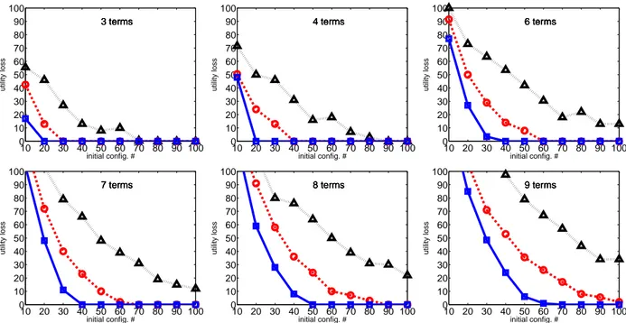
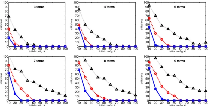
variables per term. We generate functions for the following values: {(5, 3, 3), (6, 4, 3), (7, 6, 3), (8, 7, 3), (9, 8, 3), (10, 9, 3)}. Each utility function has two terms with maximum size. Terms weights are integers selected uniformly at random in the interval [−100, 0) ∪ (0, 100]. We consider as gold standard solution the configuration obtained by optimizing the DM unknown utility function (henceforth the target utility function).
The number of catalog features is 40. The maximum size of terms is assumed to be known. Furthermore, the probability of inaccurate feedback swapping a pairwise preference is fixed to the value 0.1.
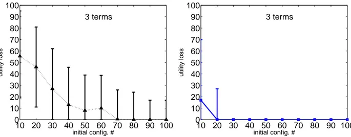
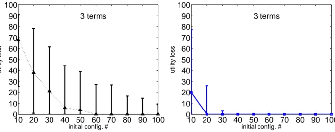
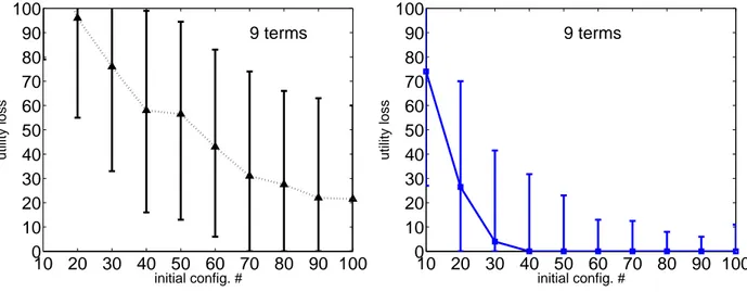
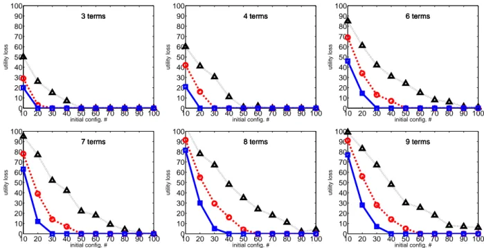
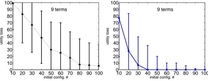
We run a set of experiments where the training set is initialized by the ranking of 10, 20, . . . 100 configurations generated by sampling uniformly at random the Boolean feature values. Fig. 3 reports the utility loss (or regret) of the best configuration, i.e., the solution optimizing the current approximation of the target utility function, at the different iterations for an increasing number s of initial configurations to be ranked. At the following iterations,
s/2 configurations are generated and their ranking is added to the training set (see Sec. 2). The utility loss is the
amount of utility lost by recommending the best rather than the gold configuration and it is measured as the difference between their respective costs (approximation error). Considering the simplest problems with three and four terms, our algorithm can identify the solution preferred by the DM at the first iteration, provided that at least 90 initial