1
ALMA MATER STUDIORUM – UNIVERSITÀ DI
BOLOGNA
CAMPUS DI CESENA
SCUOLA DI INGEGNERIA E ARCHITETTURA
CORSO DI LAUREA MAGISTRALE IN INGEGNERIA
BIOMEDICA
Titolo della tesi
“Analysis of electroencephalography signals collected in
a magnetic resonance environment: characterisation of
the ballistocardiographic artefact"
Tesi in Bioimmagini LMRelatore Presentata da
Prof.ssa Cristiana Corsi Mariangela Del Castello
Correlatori
Prof. Dante Mantini
Ing. Marco Marino
Anno Accademico 2015/2016
3
Table of contents
Abstracts ... 5
Introduction ... 7
Chapter 1 – EEG & MRI techniques ... 9
1.1 Electroencephalography - EEG ... 9
1.1.1 Electrophisiological basis of EEG ... 9
1.1.2 EEG instrumentation ... 12
1.2 Magnetic Resonance Imaging - MRI ... 14
1.2.1 Fundamental concepts of MRI ... 14
1.2.2 MRI acquisition system ... 19
1.2.3 Functional MRI ... 20
1.3 EEG – fMRI technique ... 21
1.3.1 EEG instrumentation for MR environment ... 23
1.3.2 EEG - fMRI acquisition protocol ... 24
Chapter 2 – Imaging Artefact & Ballistocardiographic artefact ... 27
2.1 Imaging Artefact ... 29
2.1.1 Method for removing the Imaging Artefact ... 31
2.2 Ballistocardiographic Artefact ... 32
2.1.2 Methods for removing the Ballistocardiographic Artefact ... 37
2.3 Thesis’s Aim ... 43
Chapter 3 – Materials & Methods ... 45
3.1 EEG – fMRI acquisition ... 45
3.2 EEG data processing ... 46
3.2.1 Removal of Imaging Artefact ... 47
3.2.2 Identification of R peaks in ECG signal ... 48
3.2.3 Identification of BCG peaks in EEG signal ... 51
3.2.3.1 Statistical analysis of RR interval and R-BCG delay relation ... 54
4
3.2.5 Evaluation of root mean square of EEG signals ... 57
3.2.6 Evaluation of field distribution maps ... 58
3.2.6.1 Cross – correlation between maps... 58
3.2.6.2 PCA of average maps ... 60
Chapter 4 – Results & Discussions ... 61
4.1 Relation between RR interval and R-BCG delay ... 61
4.2 Evaluated RMS of EEG signals ... 66
4.3 Results of cross – correlation between maps ... 68
4.4 PCA results ... 71
Conclusion ... 75
Acknowledgements ... 79
Bibliography ... 81
5
Abstract
Simultaneous recording of electroencephalography (EEG) signals and functional magnetic resonance (fMRI) imaging is a powerful approach in the field of neuroscience to study brain functions and dysfunctions. It allows obtaining information about brain functioning with high temporal resolution and high spatial resolution at the same time. The EEG technique records electrical signals of brain activity with a resolution of milliseconds. The fMRI acquisitions give information about the anatomy and the physiology of the brain with a resolution of millimeters. However, the combination of these two procedures increases the presence of artefacts in the EEG signal, thus obscuring the brain activity. The artefacts are caused by the interactions between the subject, the EEG system and the scanner’s magnetic fields. The main two artefacts are: the imaging artefact and the ballistocardiographic (BCG) artefact. The imaging artefact is caused by the gradients switching during the images acquisition. However well-performing methods for its removal have been implemented.
The BCG artefact is related to the cardiac activity of the subject and it is characterized by high variability between each occurrence. The variability is in terms of: amplitude, waveform and duration of the artefact. Several algorithms have been implemented to remove the artefact. However, because of its complex nature, the total removal of the BCG is still a challenging task. The topic of the thesis is to analyze EEG signals collected in a magnetic resonance environment and to characterize the BCG artefact. The aim is to understand additional features about it that can help to improve or create new methods.
With this work we have shown why the methods proposed in literature can lead to residual artefact in the clean EEG signal. Performing statistical analysis and using statistical tools like Pearson’correlation coefficient, we have found that the BCG artefact occurrences are characterized by a variable delay from the related R peak in the ECG, that is the referring event in cardiac activity in our analysis. Furthermore the R-BCG delay is related to the cardiac frequency: when the cardiac frequency decreases the BCG artefact appears with a larger delay after the R wave. Other findings are about the main contributions to the BCG artefact. Performing the principal component analysis on the average artefact activity across subjects, we have shown that the artefact is due to two principal contributions related to the blood flow in head vessels and its pulsatility in the major arteries in the scalp.
6
Abstract – Italian version
L’acquisizione simultanea di segnali elettroencefalografici (EEG) e immagini di risonanza magnetica funzionale (fMRI) permette di investigare connessioni e attivazioni cerebrali in modo non invasivo. Inoltre le informazioni ottenute sono caratterizzate da elevata risoluzione temporale ed elevata risoluzione spaziale. La tecnica EEG consente di registrare i potenziali elettrici provenienti dal cervello con una risoluzione temporale dell’ordine del millisecondo. L’fMRI consente di acquisire immagini descriventi anatomia e fisiologia del cervello, con una risoluzione spaziale dell’ordine del millimetro.
Allo stesso tempo però, la presenza del campo magnetico altera in modo non trascurabile la qualità dei segnali EEG acquisiti. In particolare due artefatti sono stati individuati: l’artefatto da gradiente e l’artefatto da ballistocardiogramma (BCG). L’artefatto da gradiente è causato dalla variazione dei gradienti utilizzati per la formazione delle immagini. Grazie alle sue proprietà stazionarie, l’artefatto viene rimosso in maniera efficace dagli algoritmi finora implementati.
L’artefatto da BCG è legato all’attività cardiaca del soggetto, ed è caratterizzato da elevata variabilità tra un’occorrenza e l’altra. La variabilità è in termini di: ampiezza, forma d’onda e durata dell’artefatto. Differenti algoritmi sono stati implementati al fine di rimuoverlo, ma la rimozione completa rimane ancora un difficile obiettivo da raggiungere a causa della sua complessa natura.
L’argomento della tesi riguarda l’analisi di segnali EEG acquisiti in ambiente di risonanza magnetica e la caratterizzazione dell’artefatto BCG. L’obiettivo è individuare ulteriori caratteristiche dell’artefatto che possano condurre al miglioramento dei precedenti metodi, o all’implementazione di nuovi.
Con questa tesi abbiamo mostrato quali sono i motivi che causano la presenza di residui artefattuali nei segnali EEG processati con i metodi presenti in letteratura. Attraverso analisi statistica, usando strumenti come il coefficiente di correlazione di Pearson, abbiamo riscontrato che occorrenze dell’artefatto BCG sono caratterizzate da un ritardo variabile rispetto al picco R sull’ECG, che nella nostra analisi rappresenta l’evento di riferimento nell’attività cardiaca. Abbiamo inoltre trovato che il ritardo R-BCG è legato alla frequenza cardiaca: quando la frequenza cardiaca diminuisce, l’artefatto BCG si presenta con un ritardo maggiore rispetto l’onda R. Le successive valutazioni riguardano i maggiori contributi all’artefatto BCG. Attraverso l’analisi alle componenti principali, eseguita sull’attività media dell’artefatto individuata a seguito di un’analisi inter-subjects. Abbiamo mostrato che l’artefatto è causato da due contributi principali, legati al fluire del sangue dal cuore verso il cervello e alla sua pulsatilità nei vasi principali dello scalpo.
7
Introduction
The combination of electroencephalography (EEG) technique and functional magnetic resonance imaging (fMRI) is a powerful tool for non-invasive investigation of brain function and dysfunction in presence of diseases. By using these two techniques simultaneously, it is possible to obtain information on brain activity characterized by high temporal resolution (from EEG) and high spatial resolution (from fMRI).
On the other hand, EEG signals recorded in magnetic environment are corrupted by artefactual contributions caused by the interaction between the subject, the EEG electrode assembly and the scanner’s magnetic fields. The two main artefacts are: the imaging artefact and the ballistocardiographic (BCG) artefact. The first artefact is caused by the gradients switching during the images acquisition. It is characterized by periodical and consistent occurrences, with amplitude much higher than the EEG signals. The second one is related to the cardiac activity, thus it can be identified using an ECG trace, which is recorded during the EEG-fMRI acquisition. After a QRS complex it is possible to identify a BCG occurrence in the EEG signals. The BCG artifact is caused by three effects: 1) pulse-driven expansion of the scalp due to the pulsatility of the blood, which is affecting especially the areas in correspondence of the major vessels; 2) pulse-driven rotation of the head due to the axial movement of the body after each cardiac ejection; 3) Hall effect in the head vessels due to the blood flow in the magnetic field [22,23]. The first two effects lead to the electrodes movement which, in the magnetic environment, produces an electromotive force that adds up to the EEG signals. The third contribution leads to a force (identified by Lorentz’s rule) that adds up to the EEG signals, too. The BCG artefact is characterized by high variability beat-to-beat in terms of amplitude, waveform and duration and they can vary with different magnetic field strengths. [29]
Several algorithms have been implemented for the offline removal of these artefacts. The most used methods are based on Average Artefact Subtraction (AAS) [30], Optimal Basis Set (OBS) [25] and Independent Component Analysis (ICA) [33, 34]. Each of these methods makes assumptions which cannot be easily satisfied since the BCG artefact has non–stationary features. For example the AAS and OBS based methods hypothesize that the delay between the BCG occurrence and the R peak in the ECG is constant. Whereas the ICA procedure is based on the assumption that the sources are stationary, while the BCG artefact is not stationary. Thus removing the artefact it is still a challenging task.
8
The purpose of this thesis is to analyze EEG signals recorded in a scanner for MR imaging. Focusing especially on BCG artefact occurrences, with the aim to better characterize the artefact and to understand why the implemented methods can lead to artefact residual. The analysis was performed using functions implemented in MATLAB and in the EEGLab toolbox.
The work has been conducted with the BIND (Brain Imaging & Neural Dynamics) group at the KU Leuven University in Belgium.
The thesis is composed by four main chapters. The first two chapters deal with introductive issues on EEG, fMRI and related artefacts. They will be useful for a deeper understanding of methods and obtained results which are reported in the third and fourth chapters. Specifically, the first chapter is an overview about the EEG and MRI techniques, the EEG instrumentation and the MRI acquisition system. Main concepts about EEG-fMRI approach are discussed. Furthermore, a brief description of EEG instrumentation for magnetic environment and the protocol for EEG-fMRI acquisition are reported.
The second chapter deals with artefacts and it is divided in two parts. In the first one the imaging artefact and the methods implemented for its removal are described. The second part is focused on the description of the BCG artefact, its origins and features. Moreover the main implemented methods for removing the BCG artefacts are described (like AAS, OBS, ICA) with a comparison about their performances.
The third chapter is about materials and methods. Information about the experimental EEG-fMRI acquisition, used instrumentation and parameters features is given. The methods used during the EEG signals analysis are described. Specifically, the methods used for imaging artefact removal, pre-processing steps of ECG signals and the concept of signals epoching are reported. Furthermore, statistical analysis tools such as Tukey’s method for outlier removal, Pearson’s correlation coefficient, and the using of principal components analysis are described.
In the fourth chapter the results obtained using the methods described in the previous chapter are illustrated and discussed.
In the final part conclusion and the future perspective are described.
9
Chapter 1 – EEG & MRI techniques
1.1 Electroencephalography EEG
1.1 .1 Electrophisiological basis of EEG
Electroencephalography (EEG) is a non-invasive technique that permits to reveal electrical fields produced by neurons. The EEG signal is measured on the scalp and it describes the synchronized activity of cortical neuronal populations.
The cerebral cortex is composed by six functional layers and its neurons can be divided in two groups: pyramidal neurons and non-pyramidal neurons.
Pyramidal neurons can be found in the third, fifth and sixth layers, and they are characterized by: triangular shaped soma with the apex on the top, a single axon, a large apical dendrite, multiple basal dendrites, and dendritic spines. Apical dendrites can usually extend until the superficial layer of the cortex, and they run parallel to each others, while being perpendicular to the cortical surface.
Non-pyramidal neurons are characterized by: a smaller soma compared to pyramidal neurons, short dendrites and a short axon. These neurons are also called local neurons since their axon and dendrites transmit signals only to the neighboring cells (see fig. 1).
The main contribution to the EEG signals comes from pyramidal neurons, due to the apical dendrites organization. The parallelism between apical dendrites and the synchronized activity allow measuring an electrical signal on the scalp.
Figure 1 Cortical column with pyramidal (A) and non-pyramidal neurons (B-C). The
10
At level of a single neuron, the electrical phenomena are based on the occurrence of ionic currents. There are two forms of neuronal activation: the fast depolarization of the neuronal membranes and the slower changes in membrane potential due to synaptic activation. The first one results in the generation of an action potential mediated by sodium and potassium voltage-dependent ionic conductances. The action potential generates a rapid change in the membrane potential, that varies from negative to positive while returning to the initial negative value (about -70 mV) in 1-2 ms. In this way, a pulse is generated and it propagates along axons and dendrites without any loss of amplitude.
The second ones are mediated by neurotransmitters and they can be distinguished in two kinds: excitatory postsynaptic potentials (EPSPs) and inhibitory postsynaptic potentials (IPSPs). This type of neuronal activation differs depending on the neurotransmitter and the corresponding receptor. During an EPSP the transmembrane current is generated by positive ions inwards (e.g. Na+), while during an IPSP the transmembrane current is generated by negative ions inwards (e.g. Cl-) or positive ions outwards (e.g. K+). This transmembrane current flows in or out of the neuron in correspondence of the active synaptic sites. It is important to underline that the contribution of action potentials to the signal recorded by EEG instrumentation is very low, as axons do not have a global preferential direction. On the contrary, they have different directions in the cortical space. Furthermore, the brief duration (1-2 ms) of the action potentials does not allow axons to release the signal in synchrony way. On the other hand, the higher duration (10-100 ms) of synaptic currents makes easier to add up the generated potentials even if the synchronization is not perfect. Accordingly, EEG measurements represent the expression of the post-synaptic activities of pyramidal neurons population in the cerebral cortex. [1][2]
Figure 2 Scheme of cortical pyramidal cell showing
the patterns of current flow caused by two modes of synaptic activation at an excitatory (E) and an inhibitory (I) synapse. (Adapted from [1])
11
EEG recordings show continuous fluctuations in time, which frequency and amplitude are influenced by the internal states of the subject and by the occurrence of external conditions. These fluctuations have been categorized in different groups called rhythms, based on the frequency content. It has been shown that different brain rhythms are associated to the different tasks or states.
Six types of rhythms have been observed.
Delta rhythm (δ): characterized by a frequency range between 0.5 Hz and 4 Hz and amplitude range between 20 µV and 200 µV. It is the slowest rhythm but with the highest amplitude. It is seen normally in babies and in adults during the NON-REM deep sleep. Theta rhythm (θ): characterized by a frequency range between 4 Hz and 7 Hz and amplitude range between 20 µV and 100 µV. It can be observed especially during the pre-sleep phase.
Alpha rhythm (α): characterized by a frequency range between 8 Hz and 13 Hz and amplitude range between 20 µV and 50 µV. It is seen during conscious relaxed state with closed eyes.
Mu rhythm (μ): characterized by the same frequency range as alpha rhythm, it can be observed during physical rest, but unlike the alpha rhythm, it is seen also with eyes open. Beta rhythm (β): characterized by a frequency range between 13 Hz and 30 Hz and amplitude range between 5 µV and 30 µV. It can be observed during attention and concentrating state.
Gamma Rhythm (γ) : characterized by frequencies higher then 30 Hz and amplitude range between 1 µV and 20 µV. It can be observed during cognitive function.
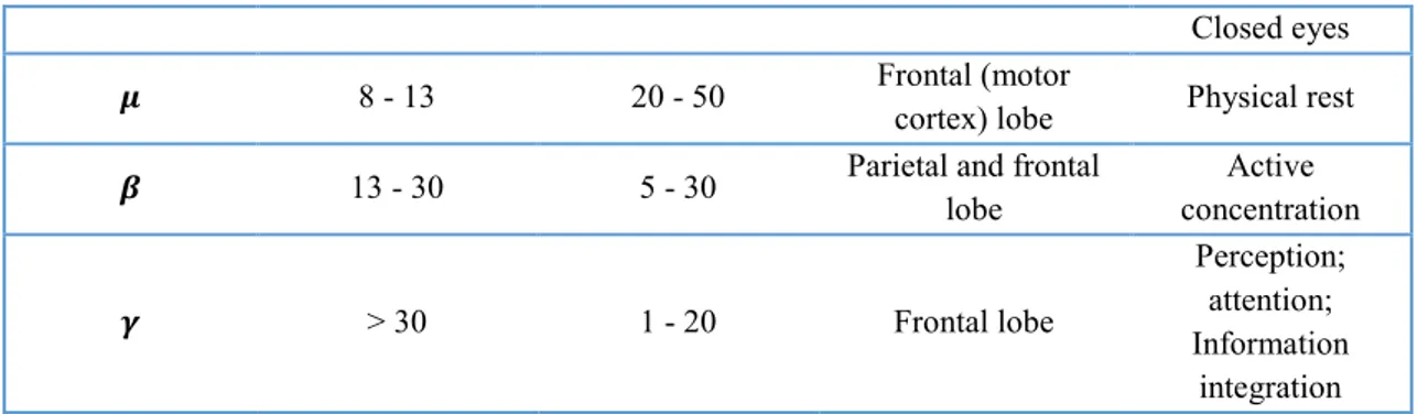
In table 1 all the features about brain rhythms are summarized. [2]
Table 1 Main features about brain rhythms
Rhythm Frequency (Hz) Amplitude (𝝁𝑽) Brain Location Brain Condition
𝜹 0.5 - 4 20 - 200 Frontal and parietal
lobe
Non – REM deep sleep; Pathological condition; Coma 𝜽 4 - 8 20 - 100 Temporal and parietal lobe Pre-sleep; Non – REM sleep; Memory and learning 𝜶 8 - 13 20 - 50 Occipital and parietal lobe Conscious relaxed state;
12
Closed eyes
𝝁 8 - 13 20 - 50 Frontal (motor
cortex) lobe Physical rest
𝜷 13 - 30 5 - 30 Parietal and frontal
lobe Active concentration 𝜸 > 30 1 - 20 Frontal lobe Perception; attention; Information integration
1.1.2 EEG instrumentation
EEG recording systems usually include a cap with multiple EEG electrodes, an amplifier, and one personal computer for acquisition and visualization (figure 3).
The electrodes are arranged in a cap that provides a partial or full coverage of the scalp, which allows to record signals from different areas of the cortex. EEG sensors can be made with different materials, even if the most used in EEG recordings are made in silver-chloride (AgCl).
In clinical settings, most commonly, EEG caps are composed by a low number of electrodes. Low-density caps were originally composed by 16 or 21 electrodes, but the number of sensors has increased across the years up to 32 and 64 electrodes (see fig.4). In
13
the recent years, high-density EEG (HD-EEG) caps have become also available, and especially used for research purposes. These caps are composed by 128 or 256 electrodes (see fig.4), which enable to achieve higher accuracy on the source localization of the recorded brain activity [3].
Figure 4Left: low-density EEG cap with an EOG electrode. Right: high-density EEG net
When the cap is set up on the subject’s head, a good contact between the surface of the electrode and the scalp is needed. To achieve it, gel or saline solutions are used to minimize the electrode impedance that can be checked on the monitor of the instrumentation. The cap can contain also extra electrodes for recording other physiological signal, e.g. electrooculographic (EOG) signal and electrocardiographic signal (ECG).
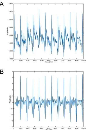
The amplitude of electrical activity on the scalp is very low (see table 1) so an amplifier is essential in order to amplify the data and make them readable [2]. By hardware and software equipment, data can be visualized in real time, furthermore initial processing of the signals can be execute, for example notch filtering. In figure 5 an example of EEG traces is illustrated.
14
1.2 Magnetic Resonance Imaging – MRI
1.2.1 Fundamental concepts of MRI
The magnetic resonance imaging is an imaging technique, that allows obtaining images of soft tissues in a non-invasive way and without using ionizing radiation.
The human body contains a high percentage of water and, therefore, high quantity of hydrogen atoms. This technique is based on the interaction between tissue’s hydrogen atoms and a magnetic field. In particular, the magnetic field 𝐵 ⃗⃗⃗ affects the hydrogen atoms’ spin. This interaction is described by the magnetic dipole moment 𝜇 ⃗⃗⃗ of the spin. When spins are in a magnetic environment, they tend to align along the field direction, in a parallel or antiparallel way. The macroscopic magnetization could be described by vector 𝑀 ⃗⃗⃗⃗ , that expresses the sum of magnetic dipole moments in the considered tissue, and it is parallel to 𝐵
⃗⃗⃗ . In the case 𝑀 ⃗⃗⃗⃗ is parallel to 𝐵 ⃗⃗⃗ , the equilibrium condition occurs, but when the protons are exposed to an electromagnetic wave, characterized by a certain frequency, called Larmor frequency, 𝑀 ⃗⃗⃗⃗ is tilted proportionally to the exposure duration (see fig. 6). 𝑀 ⃗⃗⃗⃗ rotates around the magnetic field vector, trough a movement called precession, while protons release an electromagnetic wave characterized by the Larmor frequency. Successively, the tilted 𝑀 ⃗⃗⃗⃗ returns to its original state, this movement is called relaxation. [1]
It is noteworthy that the Larmor frequency is proportional to the static magnetic field and specific for each ionic species, with a value of 42.6 MHz/T for hydrogen atoms. [5] The Larmor frequency is defined as:
𝑓 = 𝛾
2𝜋𝐵 (1)
Where 𝛾 is the gyromagnetic ratio characterizing the ionic specie, B is the strength of magnetic field.
15
Figure 6 On the left: vector M parallel and tilted to the field B. On the right: tilted M rotating around B sends out an
electromagnetic wave (Adapted from [1])
In the next paragraphs, the operating principles of the magnetic resonance imaging technique are sum up.
When the subject lies in the scanner, he is exposed to a strong static magnetic field 𝐵 ⃗⃗⃗ , which builds up a macroscopic magnetization 𝑀 ⃗⃗⃗⃗ parallel to 𝐵 ⃗⃗⃗ . An electromagnetic wave characterized by protons’ Larmor frequency and duration of few milliseconds is transmitted a radiofrequency system. A detector is switched on to recording the signals emitted by the protons.
In order to produce an image, it is necessary to perturb the alignment between the static magnetic field 𝐵 ⃗⃗⃗ and protons’ spin. Three different gradient fields along three orthogonal directions are generated, with the static magnetic field always present. In this way specific tissue portions will be excited and spatial resolution in the tissue is achieved.
The gradient in the x direction (left/right) is indicated as Gx (see fig. 7). When it is switched on, the magnetic field is modified in a way that it increases linearly in the x direction, so that the electromagnetic wave emitted by protons will have a Larmor frequency that depends on their position. This signal is processed by Fourier Transform to evaluate protons’ position from the frequency spectrum.
The second gradient is Gy in y direction (anterior/posterior), perpendicular to x direction, it is switched on when a x-coordinate is already defined (Gx switched on). The starting points of the signals from the anterior and posterior regions are different. They have different phases because they are shifted in time. So it is possible to identify different y coordinates evaluating different phases in the signal (see fig. 8).
In the z direction, that is perpendicular to the previous ones, there is the gradient Gz. It is switched on at the beginning of the experiment, by the transmission of a RF (radiofrequency) pulse (see fig. 9). With this gradient a slice is selected, and the Larmor
16
frequency is constant in it. So if a RF pulse, characterized by a certain frequency f0,, is sent the magnetization vector will be tilted only in the slice characterized by the a Larmor frequency equal to f0, while, in the other slices, the Larmor frequencies are higher or lower than f0. This process is repeated for different values of frequency in order to record multislice images datasets. [1]
Figure 7 Gradient in x direction for the frequency encoding (Adapted from [1])
Figure 8 Gradient in y direction with phase encoding (Adapted from [1])
17
As previously mentioned, the vector 𝑀 ⃗⃗⃗⃗ can be tilted by an RF pulse for a limited period and then, during the relaxation, it goes back to the equilibrium state. During the relaxation, the magnetization vector is composed by two components: the longitudinal component, that is parallel to 𝐵 ⃗⃗⃗ , and the transverse component, that is perpendicular to 𝐵 ⃗⃗⃗ .
The longitudinal component reaches the maximum value corresponding to the time constant T1, called longitudinal relaxation time, by means of a process called spin-lattice relaxation, in which free water spins transfer energy to the surrounding environment. T1 refers to the mean time for an individual spin to return to its equilibrium state. It increases exponentially until a saturation value.
The transversal component vanishes by following the time constant T2, called transverse relaxation time, which explicates a process called spin-spin relaxation, which is characterized by exchanges of small amounts of energy between free water spins. It decreases in exponential way until zero. (see fig. 10) Due to the inhomogeneities of magnetic field, the magnetization vectors rotate at different speeds, and different directions. Due to these differences, their contributions are cancelled by each other, and fast decay of the signal occurs. This fast decay implies that the effective transverse relaxation time T2*, which depends on the field inhomogeneities, can be considerably shorter than T2.
Figure 10 Trends of time constants T1 (left) and T2 (right) (Adapted from [5])
The values of T1 and T2 change between different tissues, because they depend on the constitutive molecules’ properties. In this way, it is possible to distinguish different tissues of different apparatus but also, like in the case of the human brain, different segments of the same organ, that will be characterized by different intensities in the image.
18
The MRI technique allows obtaining three different kind of images: structural imaging, diffusion imaging and functional imaging. The first and second one give information about the anatomy of the brain, the latter gives information about the physiology of the brain. They can be produced by using different exciting sequences on the tissue: gradient echo, echo planar imaging and spin echo sequence, In the next paragraphs, their main features are introduced.
The gradient echo sequence is used for functional imaging. The gradient is turned on in the x direction and the magnetic field increases linearly along it, protons at different positions precess with different frequencies, resulting in signal losses due to the dephasing of the spins. A reverse gradient is then applied, so that the magnetic field will increase in the negative x direction, and the signal builds up again. This process reduces the phase difference between spins, until the complete rephasing of the spins. When the spins are rephased they emit a signal of maximum amplitude. But the spin dephasing compensation only occurs for the gradients that are inverted, while all the other field inhomogeneities cause additional spin dephasing and thus reduce the T2* value. The time difference between the initial RF pulse and the center of the gradient echo is called echo time TE. Gradient echo images are T2* weighted and the choice of TE determines the T2* contrast. Echo planar imaging is a special gradient echo sequence that has been implemented for reducing the acquisition time. After slice-selective excitation, a series of gradient echos are acquired by successive inversions of read gradient Gx. A short gradient pulse in y-direction, called blip, is switched on between successive acquisitions. The degree of phase encoding for a specific echo is given by the initial negative gradient in y-direction and the sum of the blips up to the echo acquisition time. A full image can be constructed from the data acquired. There is only one excitation pulse, so the technique is very fast. Usually, this sequence is used for fMRI acquisitions procedure[6].
In the case of spin echo sequences, two pulses are applied: the first one tilts the magnetization vector of 90°. After recording the first signal, a second pulse tilts the magnetization of 180° and a second signals is recorded. In detail, after the first pulse, all spins are aligned and they emit a strong signal. At this point, they start to rotate with different Larmor frequencies, and different speeds. When the second pulse is emitted the spins are rotated of 180° around the axis of initial alignment. In this stage, a spin overturning occurs, which means that previously slower spins become the quicker and viceversa. After a while the spins are realigned and a second strong signal (the spin echo)
19
is emitted. Using spin echoes sequence all field inhomogeneities are compensated, for this reason it is a T2-weighted method. [1][5][7]
1.2.2 MRI acquisition system
The MRI acquisition system is very expensive and voluminous medical equipment. It has to be placed in a specific room because the static magnetic field is characterized by the so-called magnetic fringe fields, which extend many meters from the magnet itself. Thus the filed attractive effect needs to be constrained in a well-defined environment to avoid accidents (for example projectile effect of metal objects). Furthermore the static magnetic field is always present even when the system is not in use.
The MR scanner is composed by three principal components (see fig. 11):
• Magnet; • RF coils; • Gradient coils.
Other components are: RF system generator, RF system detector, gradient pulse generator, hardware and software for images acquisition. For brain imaging, extra coils are used, they are defined head coil and are fixed around the head of the subject before starting the acquisition.
20
During an MR investigation, the patient lies on a movable table that allows to move the subject inside and outside the scanner. The scanner is placed in a shielded room, because of the high strength of the static magnetic field and to avoid RF interferences with other devices outside the MR environment, while the computer for the acquisition is placed in the close control room.
Different MR scanners can be distinguished by the magnetic field strength. Nowadays, the static magnetic field has intensities from 1.5 T to 9 T. The most widespread MR acquisition systems have intensities of 1.5 T and 3 T.
Furthermore, there are different types of magnet: permanent magnet, resistive magnet and superconductive magnet. In the most recent scanners, superconductive magnets are installed. This type of magnet is constituted by superconductors materials which, at the temperature of a few Kelvin, can carry current without electrical resistance. In this way very stable magnetic field of high intensity can be generated by the current flow. In order to maintain a very low temperature for the magnet, the scanner has a liquid helium pump, called cryogen pump. A ventilation system is needed to control and maintain a good oxygen level in the room, because of the percentage of helium in the atmosphere could increase. During acquisition the gradient coils produce a very high level of noise (120 dB) so the use of headphones or earplugs is necessary for the subject in the scanner. [5]
1.2.3 Functional MRI
The fMRI technique provides functional images of the brain, which allow to understand which areas are active during a task (for example visual or auditory task) or during the resting state. [8]
fMRI is based on the fact that cerebral blood flow and neuronal activity are correlated; it detects changes in metabolic and hemodynamic signals that are indirect expression of the underlying local changes in neuronal activity.
The most commonly used fMRI contrast is the blood oxygenation level dependent (BOLD) signal [9], but it can be performed using also arterial spin labeling or injected contrast agents.
BOLD contrast relies on the use of hemoglobin as an endogenous contrast agent and this is possible because of the different magnetic properties of oxygenated and deoxygenated hemoglobin. The deoxygenated one is paramagnetic (paramagnetic materials are attracted by an external magnetic field and generate induced magnetic field in the same direction of
21
it), while the oxygenated hemoglobin and brain tissues are diamagnetic (diamagnetic materials are repelled by an external magnetic field and generate low induced magnetic field in the opposite direction of it). When neurons fire, blood releases oxygen to them at a greater rate than to inactive neurons. This is called hemodynamic response, and it causes a change of levels of oxy-hemoglobin and deoxy-hemoglobin. Thus, the magnetic field, inside the scanner, can be distorted (due to the high level of deoxy-hemoglobin) and this distortion can be detected in order to measure neuronal activity in a specific area. The distortion of magnetic field leads to a change of relaxation time constant T2* value, in the activated areas, and therefore to a difference of the signal intensity in collected images. [7] Several studies have reported that a monotonic increase in metabolic and hemodynamic responses occurs subsequent to increases in neuronal activity. But at the same time, also non-linear relationship have been found, it could depend on stimulus condition. [10,11,12]. The BOLD response appears with a certain delay, a few seconds, after the neurons activation. This is because changes in blood flow occur over a much slower timescale (hundreds of milliseconds to seconds) than changes in electrophysiological activity (milliseconds or tens of milliseconds). In the recent years, neuroscientists have been investigating the relation between the BOLD response and the underlying electrophysiological activity. For this reason, growing interest has been dedicated to the development of new methods for performing fMRI acquisitions in simultaneous with EEG recording which allow to better understand brain activations at different temporal scales (see next section 1.3). [1]
1. 3 EEG – fMRI technique
In the previous sections of this introductive chapter, general concepts about EEG and MRI technique have been discussed. In this section, the integration of the two techniques during simultaneous acquisitions will be described.
The combination of EEG and fMRI constitutes a powerful tool for the non-invasive investigation of brain functions and its dysfunction in presence of diseases. Using these two techniques simultaneously, it is possible to obtain information characterized by high temporal resolution (from EEG) and high spatial resolution (from fMRI). Indeed, the spatial resolution is about a few millimeters, while the temporal resolution is about a few milliseconds. [1,7]
22
Simultaneous EEG-fMRI allows to investigate functional connectivity of the brain, during resting state and during task-related activations. This technique was implemented for the first time in 1992 for localizing electrical sources of epileptic discharges. [13]
For integrating EEG and fMRI data, three different approaches can be adopted: 1) integration through prediction, 2) integration through constraints and 3) integration through fusion. [14]
The first approach involves the use of EEG data to form a model of the expected BOLD signal changes, by convolving the time-course of a particular component of the EEG signal with the hemodynamic response function to form a regressor. This regressor provides a prediction of the time-course of BOLD signal changes linked to the particular EEG component. Then, statistical analysis is performed in order to identify voxels in the image whose signal variation is significantly correlated with the regressor. In this way, a map identifying areas where BOLD signals are consistent with the variation of the chosen EEG components is obtained. The first studies used the power of EEG signal in the alpha-frequency band and tested for correlation with BOLD signal changes in the resting state, when alpha activity is most relevant [15]. Subsequent studies have evaluated correlations between BOLD signals and power in other frequencies bands, at rest and during task performance. [16,17]
With the second approach, integration through constraints, fMRI data are used to provide spatial constraints for localizing the sources of EEG signals. Several studies showed through separate analysis of data from the two modalities that hemodynamic activity and electrical responses were localized in the same brain areas. But this type of fusion should be performed with caution for several reasons: there may not be a corresponding BOLD response if low metabolic demand is generated by the neuronal activity responsible for a particular EEG signal; an EEG response may correlate to either a positive or negative BOLD signal making it difficult to know how to impose source constraints on the EEG. [18]
The third approach is the only one that does not perform a separate analysis of the EEG or fMRI data as first step, and it consists in the pure integration of the two signals. A proper data fusion analysis requires a common temporal forward model that links the underlying neuronal dynamics of interest to the measured hemodynamic and electrical response [14], but further work is needed before this approach can be more widely exploited.
23
1.3.1 EEG instrumentation in the MR environment
In order to perform simultaneous EEG-fMRI recordings, the EEG instrumentation needs to be MR compatible. Therefore some factors must be taken into account:
• the prevention from the introduction of ferrous materials into the magnetic environment;
• the limit of radiofrequency emissions to preserve image quality; • the presence of static and time-varying magnetic fields;
• the EEG artefact associated to the magnetic fields.
Thus the electrodes are made by nonferromagnetic materials and the amplifier is shielded in a nonferromagnetic box.
The presence of magnetic fields can induce an electromotive force Vinduced in a conductive loop. Therefore the wires in the net must be checked and that the subject should not cross its arms or legs.
This Vinduced is proportional to the rate of change of magnetic flux cutting the loop 𝑑𝐵 𝑑𝑡 and the loop area A. It can be calculated by the formula:
Vinduced = 𝐴×𝑑𝐵
𝑑𝑡 (2)
The Vinduced can introduce artefacts in the signal, therefore minimize the area of any loop formed by electrode leads is important to reduce the artefact. To achieve it, electrode leads are joined in a single point on the head and the wires are twisted together from the subject’s head to the amplifier input.
Another factor referred to the electrodes lead is the movement. Some proposed solutions are: weighing down the leads passing out of the scanner, electrodes secured by a tight bandage, head fixed by vacuum cushion.
The magnetic environment introduces two kinds of interferences that are very small in EEG recordings outside the scanner.
The first one is the pulse related interference, which is caused by cardiac-related movement of the electrodes or blood flow in the head. To remove this contribution, EEG instrumentation is supplied with additional electrodes for recording ECG signal. The ECG signal will be used to implement methods for removing this interference even if the completely removal of this interference is still a challenging issue (see chapter 3).
24
The second interference is related to the electromotive force induced in the electrode lead loops by the changing magnetic fields during the imaging acquisition. To decrease its contribution changes are required on the acquisition parameters, for example on the filtering, sampling rate and dynamic range.
Another important issue is patient safety. The presence of changing fields in fact can be dangerous for the following mechanisms:
- Eddy current heating;
- Current induced in loops formed between the electrodes leads; - Current induced along electrode leads.
Moving through the static field, a current can be induced in an electrode lead loop, flowing between electrodes and hence in the patient, but this effect is very small in a magnetic field of 1.5 T. Thus at this magnitude, additional safety measures are not required whereas they should be take.
Gradient fields induce electromotive force in electrode loops, as described before, and this force is proportional to the rate of change of magnetic flux cutting the loop and the loop area. The dominant physiological effect is neuromuscular stimulation. [19]
The RF fields can induce eddy currents in the electrodes that are much greater than those induced in human tissues but the eddy currents may result in Joule heating of the electrode. Studies about this phenomenon have demonstrated that it is more significant with a static magnetic field of 4 T.
Thus any kind of loop in the wires has to be avoid in order to do not cause heating in the patient.
[1,6,20]
1.3.2 EEG-fMRI acquisition protocol
To perform an EEG-fMRI experiment, is necessary to define a protocol able to reduce interferences on EEG signals and to guarantee subjects safety.
The experimental protocol is divided in six steps: 1. Preparing the experimental setup
25
3. Setting subject up inside the MR scanner 4. Recording signals and images
5. Debriefing the subject
6. Clearing up at the end of experiment
1. Preparing the experimental setup
Set up the EEG equipment in the control room; ensure the workspace for recording the data is set to the highest temporal resolution available and correct filter settings (data can be collected with a sampling rate of 1kHz and filtered with a 0.016-250 Hz band pass filter). Set up the MR scanner in the conventional way and turn on the synchronization of the scanner and EEG clocks. Check if the synchronization is successful. Set up the TR of MR sequences to a multiple of the EEG clock period (this is necessary for a good removal of imaging artefact, see chapter 3).
2. Preparing subject
Before starting to set up the EEG cap on the subject, it is important to explain him/her the aim of the experiment and what will happen. Ask the subject to fill out the forms, in which the MR scanning safety rules and constrains are presented and to sign them. In this way, the subject consents to participate to the experiment. At this point start the procedures for the placement of the EEG cap: measure the head-circumference and select the appropriate sized cap. Place the cap on the head starting at the front of the head and pulling backwards. Positioning the cap such that Cz electrode (the vertex reference) is sited half way between the nasion and inion and also centered left-right. The electrodes’ impedance must be checked. The electrode (or electrodes) for the detection of ECG signal needs to be placed on the back or on the chest.
3. Setting subject up inside the MR scanner
Take the subject into the scanner room and ask him/her to lie on the scanner bed. The subject has to wear earplugs, headphones, because of high noise level caused by switching gradients. Arrangement of head coil over the subject’s head. The EEG cables must leave the head coil along the shortest path possible. At this point, subject’s head must be pad in order to minimize head movement. Attach the EEG cap to the amplifier, which is connected to the instrumentation by fiber optic cable, in the control room. There must not be wire loops in the EEG leads (as these can lead to RF heating and also cause larger EEG artifacts
26
to be induced) and that the cabling needs to be isolated from MR scanner vibrations as much as possible.
4. Recording inside the scanner
Switch off the helium pump during data acquisition. Before starting to acquire EEG data and scanning, the software for the EEG signals acquisition needs to be test if it is working well (for example asking to the subject to move the head, close and open eyes).
5. Debriefing the subject
When the acquisition is completed, take the subject out of the scanner and help him/her to take off the EEG cap.
6. Clearing up at the end of experiment
At the end of the acquisition, these steps are needed: check out of the participant, pack up the EEG equipment, cleaning the EEG cap (usually using water and disinfectant mixture). [7, 19, 21]
27
Chapter 2 – Imaging Artefact & Ballistocardiographic Artefact
Simultaneous recording of EEG signals and MR images is a powerful approach in the field of neuroscience. It allows obtaining information about brain functioning with high temporal resolution and high spatial resolution at the same time.
However, the combination of these two procedures increases the presence of artefacts in the EEG signal, thus obscuring the signal of interest. The artefacts are caused by the interactions between the subject, the EEG electrode assembly and the scanner’s magnetic fields.
The main causes of EEG artefacts in the scanner are: 1) gross movements in the static field, 2) the ballistocardiogram (BCG) and blood flow effects in the static field associated with the subject’s cardiac activity, 3) the changing fields applied during MRI images acquisition [22,23], 4) scanner vibration, 5) vibration due to the helium pump. [1]
The artefact associated to the scanner and helium pump vibrations can be attenuated by some precautions (see section 1.3.2). On the other hand artefact sources related to the cardiac activity and to the gradients switching need to be post-processed and big efforts have been done to implement methods for their removal. This chapter focuses on the imaging artefact and the BCG artefact (see fig. 12). Their origins and their removing methods will be henceforth presented.
28
Figure 12 (a) EEG signals corrupted by imaging artefact. (b) EEG signals after imaging
artefact removal but corrupted by ballistocardiographic artefact. (c) ECG trace (Adapted from [34])
29
2.1 Imaging Artefact
Many studies were performed in the past twenty years for characterizing and removing the imaging artifact. In the next paragraphs, the main findings about this artifact will be introduced.
Imaging artefact is induced by magnetic fields applied during images acquisition. Two different fields are applied: RF and gradients (Gx, Gy, Gz)(see chapter 1, section 1.2.1). The artefact is characterized by: 1) consistent waveforms, each peak component corresponded precisely to an RF and gradient pulses; 2) the artefact associated to the gradient pulse has its amplitude in the order of 103-104 𝜇V, while the amplitude of the artefact generated by the RF pulse can be up to 102 𝜇V; 3) an artefact component caused by one gradient pulse consisted of a pair of peaks, one of which deflected positively or negatively and the other inversely, thus the artefact from one gradient pulse has the differential waveform of the corresponding gradient pulse; 4) artefact induced by RF has a much higher frequency then EEG. While the gradient artefact is characterized by components in the EEG frequency range. (see fig. 13) [23]
The amplitude of induced gradient artefact is given by Faraday’s law (chapter 1).
Imaging artefact depends on scanning process, which is a preprogrammed process, thus this artefact has a strong deterministic component. The relative polarity and amplitude of the artefact varies across EEG channels, but the timing of the rising and falling edges are the same across channels. This repeatability allows to efficiently remove the imaging artefact, by subtracting an artefact template from the EEG signals.
30
Figure 13 (A) Timings of RF emission and gradients pulses in an fMRI sequence. RF, radiofrequency
wave; Gs, slice selection gradient; Gp, phase encoding gradient; Gr, readout gradient. a, Fat suppression pulses (1-3-3-1 pulses); b, slice selection RF; c, d, h, spoilers; e, slice selection gradient; f, dephasing and rephasing gradient; g, readout gradient. (B) Schematic diagram of whole EPI (echo planar imaging) sequence. (C) Imaging artefact waveform for one slice scan on a dummy EEG record with a phantom using the EPI sequence. The artefact corresponding to each gradient component described above in (A) can be identified, and it is denoted by the same alphabet as the one denoting the original gradient but with a prime. [23]
31
2.1.1 Method for removing the Imaging Artefact
The most used method for imaging artefact removal is based on the averaged artefact subtraction (AAS) and was proposed by Allen et al in 2000 [24]. The deterministic characteristics of the artefact allow constructing channel specific artefact templates, so this approach assumes that the shape of the gradient artefact does not change rapidly and that is not correlated with the physiological signal.
The artefact template is calculated channel by channel by averaging EEG epochs. The number of epochs is related to the TR of the sequence used for the acquisition in the scanner. Recording a marker in correspondence to each image acquisition occurrence is needed to identify the epochs.
Thus, the EEG signals are divided into epochs, each epoch containing an MRI volume or scan acquisition period. The epochs are then interpolated (for example by a sinc function with a factor of 10-15 [24]) and then aligned by maximizing the cross-correlation to a reference period. The epochs are averaged in order to obtain the template, which is subtracted from each epoch. In figure 14 the results are illustrated.
The most of the methods that have been proposed by researchers for correcting the imaging artifacts are based conceptually on the AAS. The several proposed algorithms differ with respect to the number and selection of averaging epochs and their weighting. [1]
Although subtraction of averaged artefact removes a large portion of the imaging artefact, residual artefact could be sometimes still present. There are two main causes for this: 1) jitter between the EEG sampling and scanner time frames; 2) differences between individual epochs and the average artefact, due to small subject movements. Allen et al.
Figure 14 (A) EEG signals recorded in the scanner. (B) Averaged
imaging artefact. (C) the result of subtracting the averaged imaging artefact in B from the EEG in A. (adapted from [24])
32
[24], in order to attenuate the residual artefact, applied an adaptive noise cancellation (ANC) filtering procedure.
However, to attenuate residual artefacts, it is also important the instrumentation for recording the EEG signals, because without a suitable acquisition, the artefact features can be lost or changed and this could cause a bad removal (see chapter 1, section 1.3.2). [24][25]
2.2 Ballistocardiographic Artefact
The Ballistocardiographic (BCG) artefact is related to the cardiac activity of the subject. Since it arises from slight electrode movements in the static magnetic field, it can be observed in absence of scanning for the images acquisition [22]. The movement could be due to the local effect of pulsatile movements of scalp vessels on adjacent electrodes (ballistic effects). This effect is called pulse-driven expansion. The pulsatile movement can cause the expansion of the scalp, especially in areas on the major vessels (e.g. the temporal artery). [26]
Another contribution to the BCG is induced by cardiac pulse-driven rotation of the head in the strong static magnetic field of the MR scanner. This rotation is driven by changes in the momentum of blood as it is pumped by the heart and shunted into the head arteries. [27] Motion of blood in arteries and veins can induce Hall effect and, thus, give another contribution to the BCG artefact. The ions in a conducting fluid, such as blood, experience a force when the fluid flows in an applied magnetic field. The force is given by
𝐹 = 𝑞𝒗×𝑩 (3)
where q is the charge of the ion, v is the flow velocity, and B is the applied magnetic field. Thus, any ions with a component of motion orthogonal to the magnetic field will experience a force whose direction is orthogonal to the plane containing both the velocity and magnetic field vectors. Positively and negatively charged particles move in opposite directions, accumulating on the vessel wall until equilibrium is established. The charge distribution on the vessel also produces an external field that causes current flow in the surrounding conducting tissue. A scalar potential is consequently produced at the surface of the body and detected, for example, by surface electrodes as used in EEG measurements. The resulting potential is proportional to the blood velocity and it is expected to show a periodic variation through the cardiac cycle. [27,28]
33
Although the artefact is mainly caused by these three effects, it is still not clear which is the degree of contribution from each of them even if, probably, the major contribution comes from the pulse-driven rotation [27,29]. These causes were identified using computational models, in parallel with acquisition in vivo, and recordings of EEG signals in vivo adopting different strategies to diminish the described mechanisms and obtaining signals with a lower contribution of BCG artefact [27, 28]. For example Mullinger et. al [27] used a bite-bar and vacuum cushion to restrain the head and observed greatly attenuating contribution of cardiac-driven head rotation.
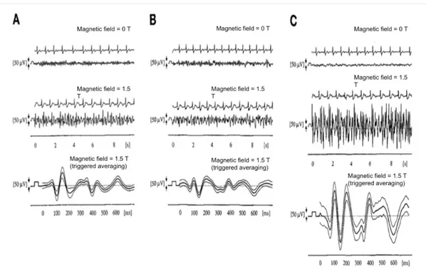
It is a matter of fact that this artefact is related to the cardiac activity, thus to studying it, an electrocardiographic (ECG) signal is usually recorded during the EEG-fMRI acquisition. One or two electrodes of the cap are employed to measure the ECG signal and they are attached either on the back or in correspondence of the left side of the heart of the subject [21]. In figure 15, some EEG recordings affected by the BCG artifact are illustrated.
Figure 15 Simultaneous recording of EEG and ECG in one subject, at (A) occipital (Pz-Oz), (B) parietal (P3-O1), and
(C) frontal (F3-Fp1) electrode positions. Upmost rows show ECG and EEG recording outside the magnet. The two traces in the middle show the signals in the same volunteer inside the magnet at identical electrode positions. The lowest trace presents the EEG recording, averaged by ECG triggering (curves are mean ± 1 SD). (Adapted from [22])
Müri et al. [22] observed that there was a large difference between EEG signals recorded outside and inside the scanner. For signals detected in the static magnetic field, after a
34
certain delay from the QRS complex in the ECG, specifically after the R wave, a high contribution added up to the EEG signal and the amplitude was much larger than the amplitude outside the scanner. Furthermore, the amplitude changed across the scalp. For example, signals recorded from the frontal electrodes showed a large magnitude compared to the signals recorded in the occipital and parietal electrodes. In the study, the authors supposed that the pulse-related head movement was greater at the front of the head compared to the rear, which rests on the scanner table and under the head coil. The adherence of the electrodes with the scanner table decreases the electrodes movement and therefore the BCG artefact contribution, as shown in successive study. [28]
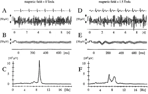
Figure 16 EEG signal at the occipital (Pz-Oz) electrode position, (A)-(C) outside the MR scanner, (D)-(F) inside the
scanner. Rows (A) and (D) show simultaneous ECG and EEG recordings. The curves in (B) and (E) represent mean ± 1 SD of the EEG recording, averaged by ECG triggering. Rows (C) and (F) display the power spectra obtained by fast Fourier transformation of (A) and (D), respectively. The additional peak at 7 Hz in the Fourier transformed signal recorded in the magnet indicates additional components. (Adapted from [22])
In the same study [22], a variation in the frequencies range was observed. In particular, additional peaks in the power spectra were found confirming the presence of additional components in the EEG signals (see fig. 16).
In later studies, the BCG artefact was deeper investigated, observing that it could be composed by several peaks, with different delays from the R peak from the ECG and with different amplitudes. It is characterized by strong variability in terms of: amplitude of BCG
35
peaks, morphology of the artefact and time occurrences of the BCG peaks. The delay between the R peaks and the first strong peak of the artefact in the EEG traces has been estimated of approximately 200 ms. [30]
It has been supposed that the first peak could be associated to the pulse-driven expansion movements while the second one to the pulse-driven rotation (see fig. 17). [29]
Figure 17 A model illustrating two contributions to the BCG. The left-hand side of the figure indicates a participant in
supine position in a MRI scanner. The polarity of the BCG artefact depends on the direction of the static magnetic field, which is different for MRI scanners from different manufacturers. The upper right- hand side of the figure illustrates the time course of blood flow over the cardiac cycle. Shown below is a single EEG trial at two left and right hemisphere electrodes (F7, F8), and the corresponding ECG trace. Note the systematic polarity reversal over time during the ejection phase of the cardiac cycle, indicated by a grey background. The lower right-hand part of the figure shows the evoked ECG traces. (Adapted from [29])
36
The amplitude of the BCG artefact can be comparable to or higher than the one the of brain signal. The BCG artifact amplitude can be in the range of 50-200 𝜇𝑉, or even more, and the frequencies are overlapping with the frequency range of the brain activity, as showed in figure 18. However, it is noteworthy that the amplitude of the artefact strongly depends on the magnitude of the static magnetic field. Debener et al. [29] recorded EEG signals in static magnetic field of 1.5 T, 3 T and 7 T. They found that the amplitude of the BCG artefact scaled approximately linearly with the static magnetic field strength (see figure 18). Furthermore, they also found that the spatial variability increased at higher field strength, as a consequence of the increase in the absolute magnitude of the BCG. In other words, the topographical variability of this artefact was less pronounced at 1.5 T compared with 3 and 7 T. This information is relevant for an appropriate removal of the artefact.
Figure 18. (A) Comparison of outside the
scanner (grey) and inside 1.5 T MRI scanner single-trial GFP traces, expressed as standard deviation (STD) over time, with 0 ms denoting the onset of the ECG R wave. Colour-code of mean traces is shown in D. (B) Same comparison as in A, for 1.5 T (grey) and 3 T (black) data. (C) Same comparison as in B, for 3 T (grey) and 7 T (black). (D) Group mean GFP (± standard error of the mean), overlaid for recordings outside the scanner (0 T) and at 1.5 T, 3 T and 7 T. Peak latencies are indicated for the 7 T mean GFP data. (Adapted from [29])
Furthermore, the static magnetic field has an influence on the polarity of the BCG peaks. In particular, the polarity is opposite between left and right hemispheres and it would reversed in a field with opposite direction. (see fig. 18) [29]. If the static magnetic field has a head to foot direction, the highest peak of BCG are positive on electrodes located in the left hemisphere and negative in the ones located in the right side of the head [31].
37
Due to the very high variability of the BCG artefact and its complex contribution to the EEG signals, a detailed characterization is required. An appropriate evaluation of this artifact features can provide an important basis for developing methods for properly removing it from the EEG recordings and recovering the information about brain activity from the cleaned EEG signals.
2.2.1 Methods for removing the BCG Artefact
So far several methods have been proposed to reduce the BCG artefact and to improve the EEG signals quality.
The methods, which will be presented in detail in the following paragraphs, are based on different procedures:
• Average Artefact Subtraction (AAS); • Principal Component Analysis (PCA); • Independent Component Analysis (ICA).
Method based on Average Artefact Subtraction
The first method was implemented by Allen et al. in 1998 [30]. They introduced the AAS algorithm. This method relies on the hypothesis that the artefact is relatively stable across a number of successive heartbeats. The algorithm’s aim is to create a template of the artifact to be subtracted from the EEG signals. The idea is similar to the one implemented for removing the imaging artifact, with the difference that the epoching of the data is performed by using as triggers the information from the ECG signal.
The first step of the algorithm consists in the identification of the ECG peaks, i.e. the R peaks of the QRS complex. Then, a template is calculated by averaging the epochs of the R peaks triggered EEG signals. Finally, the template, specific for each channel, is subtracted epoch by epoch.
More in detail, the EEG signal is epoched channel by channel, and each epoch is defined as a time window centered on the R peaks instant and having as length the mean R-R interval. This time interval is necessary because the BCG peak normally occurs a short time after the QRS complex (see previous section), this delay was assumed equal to 210 ms. The
38
epochs are averaged (removing epoch that contains other artifacts), obtaining the artefact template that is subtracted from EEG signal (see fig. 19). The procedure can be implemented also in real time.
Figure 19 This shows a schematic view of the BCG subtraction method. (A) An ECG peak corresponding to a QRS
complex is detected. (B) BCG waveforms in the EEG channels, time-locked to the ECG peaks are averaged. (C) The averaged BCG signal for each channel is subtracted from the EEG signals at times corresponding to the ECG peaks. (D) To confirm that an ECG peak detection corresponds to a QRS complex, an averaged QRS waveform is calculated from the first four ECG peak detections with temporal characteristics which indicate a high probability of being QRS complexes. This is then cross-correlated with the ECG waveform at each peak detection. (E) ECG peaks corresponding to noise in the ECG signal are rejected due to a low value of cross-correlation with the averaged QRS waveform calculated in D. (F) QRS complexes which are not detected by threshold crossing are added. (G) The sections of EEG (duration ± half the mean R–R interval) occurring a short time interval after the ECG peaks are averaged. A time interval is necessary as the peak of the BCG in an EEG channel normally occurs a short time after the QRS complex. (H) If the section of EEG time locked to an ECG peak contains other artifacts, the section is excluded from the average BCG waveform. (Adapted from [30])
The quality of the template should increase with the number of epochs used, but averaging more epochs could reduce the sensitivity of the template to capture temporal fluctuations of the artefact. Furthermore, this method cannot take into account of the large variability of the BCG artefact, as previously described, thus it leads to non-negligible residual artefact after the subtraction.
Also, the choice of the template length may be problematic due to the variations in the R-R interval, as the subject’s heart rate is variable. Consequently, mismatch between template
39
window length and artefact duration would lead to residual artefacts. So different strategies have been proposed for a better generation of the template, for example by using weighted averages or median instead of the mean values. [30]
Methods based on Principal Component Analysis
Another algorithm that improves the quality of EEG signals, removing the BCG artefact, is based on Principal Component Analysis (PCA). The PCA is a statistical procedure that uses an orthogonal transformation to convert a set of observations of possibly correlated variables into a set of values of linearly uncorrelated variables called principal components. The number of principal components is less than or equal to the number of original variables. This transformation is defined in such a way that the first principal component has the largest possible variance (the highest content of information). The other components are orthogonal to the first one and between them and the associated variance has decreasing value from the first to the last component.
The method is called Optimal Basis Set (OBS) [25], and it differentiates from the AAS for the different artefact template generation. The assumption is that over a sufficient period of EEG recording from any single EEG channel, the different BCG artefact occurrences in that channel are all sampled from a constant pool of possible shapes, amplitude and scales. Furthermore, each occurrence of a BCG artefact, in any given EEG channel, is independent of any previous occurrence. The principal components of all occurrences can then describe most of the variations of the BCG artefact in that channel. The PCA is applied on a matrix of BCG artefact occurrences, channel by channel. This method takes into account a constant delay between the R peaks in ECG signal and BCG peaks in EEG signal of about 210 ms, as proposed by Allen et al. [30].
In the current paragraph the main steps of this method are summarized. First of all, after the detection of the R-peaks from the ECG, the R peaks are shifted forward in time by 210 ms in order to identify the BCG occurrences in the current EEG channel. Then, in the second step, for each channel, all BCG artefacts occurrences are aligned in a matrix and PCA is performed. The optimal basis set is made up of the first three or four principal components [32]. The OBS is then fitted to, and subtracted from, each BCG artefact occurrence. The process is repeated for each channel.
40
Thus this approach, unlike AAS, can take into account for greater temporal variation in the artefact shape, leading to lower quantity of residual artefact than AAS procedure, as shown in figure 20. [25]
Figure 20 Plot illustrating the amount of BCG artifact residuals left by the AAS and OBS methods. The height of each
bar is the percentage of the original BCG artifact power for that channel that still remained as residuals after cleanup. The shown results are the average over 8 data sets. On average using OBS left 2.7% residuals while AAS left behind 4.0% of the original BCG artifact power. (Adapted from [25])
Methods based on Independent Component Analysis
The Independent Component Analysis (ICA) is a signal processing technique that can be used to recover independent sources from a set of simultaneously recorded signals that result from linear mixing of the source signals. Accordingly, the methods based on the ICA hypothesize that the BCG artefact contribution is physiologically independent from ongoing EEG activity, since the generator of the artefactual activity comes from the cardiac pulsation and not from neurophysiological source.
Unlike the previous described methods, ICA technique does not make assumptions about the shape of the source signal, but the assumption is that the sources are supposed to be stationary in time and space.
When applying the ICA on an EEG dataset, the output is composed by a number of components, equal to the number of the EEG signals given as input. Since, these components are independent, some of them are associated to artefactual activity, while others to brain signal. It can be difficult to visually identify and select the components that represent the BCG artefact because their number and shape are not precisely defined. The


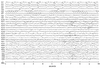
![Figure 23 Artifact-free EEG data reconstructed using ICA with the traces in fig. 22.(Adapted from [34])](https://thumb-eu.123doks.com/thumbv2/123dokorg/7421229.98952/42.892.201.686.672.1008/figure-artifact-free-eeg-reconstructed-using-traces-adapted.webp)