UNIVERSITA' DI BOLOGNA
SCUOLA DI SCIENZE
SECOND CYCLE DEGREE in
ENVIRONMENTAL ASSESSMENT AND MANAGEMENT,
Curriculum Climate KIC
Automatic methods for crop classification by merging
radar (Sentinel1) and optical (Sentinel2) satellite images and
Artificial Intelligence analysis
Thesis in Environmental, Political and Economic
Management Systems
Relatore
Prof.re Andrea Contin
Correlatore
Dott.re Nicolas Greggio
Controrelatore
Dott.re Alessandro Buscaroli
Academic year 2018-2019Presents
Beatrice Gottardi
Index
1 INTRODUCTION ... 7
1.1 REMOTE SENSING FOR EARTH OBSERVATION, LAND USE AND LAND COVER ... 7
1.2 THE COPERNICUS PROGRAMME ... 11
1.3 CLASSIFICATION OF THE ELECTROMAGNETIC SPECTRUM ... 13
1.4 USE OF WITH ARTIFICIAL INTELLIGENCE ... 15
1.5 PIXEL BASED VS PARCEL BASED CLASSIFICATION ... 20
1.6 STUDY GOAL ... 21
2 STUDY AREA AND DATA ... 23
2.1 STUDY AREA ... 23
2.2 MATERIALS AND DATA ... 25
2.2.1 FIELD DATA ... 25
2.2.2 THE GOOGLE EARTH ENGINE ... 27
2.2.3 SENTINEL1: SAR SENSOR ... 29
2.2.4 SENTINEL2: MSI, MULTISPECTRAL INSTRUMENT ... 31
3 METHODS ... 33
3.1 PRELIMINARY DATA PROCESSING ... 33
3.1.1 BRP DATASET ... 33
3.1.2 SENTINEL1 DATA ... 34
3.1.3 SENTINEL2 DATA ... 35
3.2 MULTITEMPORAL ANALYSIS: GAP FILLING (SPATIAL AND TEMPORAL FILLING) ... 36
3.3 RANDOM FOREST CLASSIFIER AND ACCURACY ASSESSMENT ... 39
3.4 SUMMARY OF THE WORKFLOW ... 40
3.5 PREDICTIONS ... 41
4 RESULTS ... 42
4.1 VALID OBSERVATIONS ... 42
4.4 ACCURACY ... 45
4.4.1 TRAINING ... 45
4.4.2 TESTING ... 46
4.5 RESULTS USING ONLY THE SENTINEL1 IMAGERY ... 49
4.5.1 RFC MODEL FOR 2018 ... 49 4.5.2 PREDICTION FOR 2019 ... 51 4.6 COMPARISON OF THE DIFFERENT RFCS ... 52 5 DISCUSSION ... 54 6 CONCLUSIONS ... 59 7 BIBLIOGRAPHY ... 61 8 ANNEXES ... 66 9 ACKNOWLEDGMENTS ... 68
ABBREVIATIONS AAN Agricultural Area of the Netherlands ACC Accuracy ANN Artificial Neural Network API Application Programming Interface AQ60 Cloud Bitmask for Sentinel2 BSI Bare Soil Index BRP Basic Registration of crop Plots CAP Common Agricultural Policy CCRS Canada Center for Remote Sensing CNN Convolution Neural Network DL Deep Learning EM ElectroMagnetic EO Earth Observation ESA European Space Agency ETM+ Enhanced Thematic Mapper Plus EUMETSAT Exploitation of Meteorological Satellites GEE Google Earth Engine GRD Ground Range Detected IDE Integrated Development Environment IW Interferometric Wide KNN K-Nearest Neighbours LPIS Land Parcel identification System ML Machine Learning MSI Multi-Spectral Instrument (MSI) MV Microwave electromagnetic spectrum NASA National AeroSpace Administration NDVI Normalized Difference Vegetation Index NIR Near Thermal Infrared electromagnetic spectrum OA Overall Accuracy OLI Operational Land Imager OOB Out-Of-Bag
RA Random Accuracy RF Random Forest RFC Random Forest Classifier RS Remote Sensing SAR Synthetic-Aperture Radar SR Surface Reflectance SSD Spatial Sampling Distance STOWA Foundation for Applied Water Management Research in the Netherlands SVM Support Vector Machine SWIR ShortWave InfraRed electromagnetic spectrum TIR Thermal Infrared electromagnetic spectrum TIRS Thermal Infrared Sensor TOA Top-of-Atmosphere VI Vegetation Index VIS Visible electromagnetic spectrum
1 Introduction
Human primary needs for food, water, fuel, clothing and shelter must be met from the land, which is in limited supply. As population and aspirations increase, land becomes an increasingly scarce resource. Studying land use and land cover is important to make the best use of this limited resource.
Land use must change to meet new demands. However, land use changes bring up conflicts between competing uses, i.e. between the interests of individuals and the common good. Land covered by towns and industry is no longer available for farming. Likewise, the development of new farmland competes with forestry, water supplies and wildlife.
Land-use planning is the systematic assessment of land and water resource, the development of options for land use and the study of the socio-economic conditions in order to select and adopt the best land-use choices (Sicre, et al., 2020). Its purpose is to select and put into practice those land uses that will best weight the needs of people and the protection of resources for future generations. The driving forces in planning are the need for improved management and the need for a different land uses due to changing circumstances. Planning to make the best use of land is not a new idea. Over the years, farmers have made plans, season after season, deciding what to grow and where to grow it. Their decisions have been made according to their own needs, their knowledge of the land and the technology, labour and capital available. As the size of the area, the number of people involved and the complexity of the problems increased, so did the need for information and rigorous methods of analysis and planning (FAO, 1993).
1.1 Remote sensing for Earth Observation, Land Use and Land Cover
Earth Observation (EO) is the gathering of information about planet Earth’s physical, chemical and biological systems via remote sensing technologies, usually involving satellites carrying imaging devices. EO is used to monitor and assess the status of, and
reliable and repeat-coverage datasets, which, combined with research and the development of appropriate methods, provide a unique mean for gathering information concerning the planet. Examples include the monitoring of the state and evolution of our environment, be it land, sea or air, and the ability to rapidly assess situations during crises such as extreme weather events or during conflicts (European Commission, 2016).
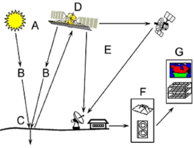
Remote sensing by imaging systems consists in a process where the interaction between incident radiation and the target of interest is involved. The following seven points, well explained in the “Fundamental of Remote Sensing” by CCRS (Canada Center for Remote Sensing, 2015), shortly describe the process. In Figure 1, the whole procedure is represented.
Figure 1: Picture representing the elements of a remote sensing system. (Canada Center for Remote Sensing, 2015)
1. Energy Source or Illumination (A). The requirement number one for remote sensing is to have an energy source which provides electromagnetic energy to the target of interest. The energy source could be the Sun (passive remote sensing, e.g. optical satellite) or a wave emitted by the satellite (active remote sensing, e.g. radar satellites). Also, the direction of the electromagnetic radiation is used to gather information.
2. Radiation and the Atmosphere (B). On the way from source to target, the wave will interact with the medium it passes through. This interaction may take place a second time as the energy comes back to the source and is detected. Part of the electromagnetic wave could be absorbed so that it does not reach the ground, or the reflected wave
could be absorbed so that it does not reach the detector. It is important to identify the so-called “atmospheric windows” to define the characteristics of the sensors on board, and to create specific filters. In the analysis of the data, these interferences between the atmosphere and the wave have to be removed, e.g. with atmospheric correction and cloud filters (more details in section 3.1).
3. Interaction with the Target (C). The radiation interacts with the target depending on the properties of both the target and the radiation. Part of it can be absorbed, reflected, scattered or its wavelength modified.
4. Detection and Recording by the Sensor (D). After the energy has been scattered by, or emitted from, the target, a sensor is required to collect and record the radiation. 5. Transmission, Reception, and Processing (E). The detected signal has to be transmitted, often in electronic form, to a receiving and processing station where data are translated into an “image”, i.e., a collection of information which includes images but also other data or meta-data about the collected radiation (polarisation, direction, etc.). 6. Interpretation and Analysis (F). The processed image is interpreted, visually and/or digitally, to extract information about the target. This step allows converting an image into physical measurements. The conversion is performed using calibration and cleaning from background noise.
7. Application (G). Finally, the information extracted from the collection of images, called “imagery”, describes some target properties, assist in solving a particular environmental problem or describe processes.
The study described in the thesis mainly falls into the last point of the process.
Recently, the improvement of remote sensing for EO allowed the development of better monitoring and a better description of the changes in the Earth surface. A great amount of data has been stored and data analysts are working together with physical earth systems scientists in order to analyse this information. Traditional physical models are no more the only prediction methods which can be applied: artificial intelligence is now supporting big data analysis and extrapolations. For example, satellite images have been largely exploited for mapping continental areas (Hościło & Lewandowska, 2019), for
analysing crops (Kristof Van Tricht, 2018; Sicre, et al., 2020), for estimating biophysical parameters (Betbeder, et al., 2016), etc.
The exploitation of multispectral optical sensors to identify differences among various vegetation types (see section 2.2.4) has various proven methods, e.g. using vegetation indexes (Nathalie Pettorelli, 2005; Xingwang Fan, 2016). However, cloud-free or weather independent data are necessary to map cloud-prone regions. Very recently, given the complementary nature of optical and radar signals, notably their different penetration capacities (see section 2.2.3), they have been used in synergy to improve performances in agricultural land monitoring (Steinhausena, et al., 2018). Moreover, vegetative cover is characterized by strong variations within relatively short time intervals. These dynamics are challenging for land cover classifications but deliver crucial information that can be used to improve the performances of a machine learning algorithm that detects earth’s surface differences. Studying the time variability of the collected data may provide useful information both for understanding differences among crops and variability over the phenology of the plant (Bargiel, 2017; Kristof Van Tricht, 2018).
Satellite images are heavy datasets that can be difficult to handle, particularly on local workstations, when artificial intelligence algorithms are developed and applied. This has been a hurdle that had to be overcame in order to allow open and free access to these types of datasets and permit a knock-on disrupting added value to worldwide users, from policy makers to commercial and private users. A new tool, launched by Google in 2014, called Google Earth Engine (GEE), allows “computing in the cloud” and fast visualisation of the results. Since 2017, it has started to receive more and more interest, as a promising interface to analyse satellite images for environmental assessment and for crop mapping (Fuyou, et al., 2019), decreasing the need for computing time on local machines.
Satellite data are a valuable source for land use and land cover mapping (European Commission, 2016). Land use and land cover maps can support the understanding of coupled human-environment systems and can provide important information for environmental modelling, water resources, food waste management and new bioenergy resources implementation.
Many different campaigns have been fostered from Countries, private and public companies all over the World, for both space and ground sectors. In the last decades, NASA from USA and ESA from EU have acquired a crucial role in aerospace innovation and research, producing a relevant amount of data and making them available openly to scientists. In particular, the Copernicus Progamme launched by ESA, provides a unique combination of free access, high spatial resolution, wide field of view and spectral coverage. It represents a major step forward compared to previous missions. Therefore, the use of these new data sources may increase the quality of final crop mapping results.
1.2 The Copernicus Programme
Copernicus is the European Union’s Earth Observation and Monitoring programme, looking at our planet and its environment for the ultimate benefit of all European citizens. Thanks to a variety of technologies, from satellites in space to measurement systems on the ground, in the sea and in the air, Copernicus delivers operational data and information services openly and freely available for a wide range of application areas.
Figure 2: The Sentinels, the six missions launched till 2019 from Copernicus Programmed (source: ESA)
foster job creation. Due to its boost to many real applications that can support decision makers and new start-ups, this Programme has a high potential for the general public. As described in the European Commission Report “Europe’s Eyes on Earth” (2015), the ‘’Copernicus programme is supported by a family of dedicated, EU-owned satellites (the Sentinels) specifically designed to meet the needs of the Copernicus services and their users”. Since the launch of the first satellite – Sentinel-1A – in 2014, the European Union set in motion a process to place a constellation of more than a dozen satellites in orbit during the next ten years (see Error! Reference source not found.).
The Sentinels “fulfil the need for a consistent and independent source of high-quality data for the Copernicus services’’ (European Commission , 2015). These satellites are equipped with different sensors on board, able to detect different features of air, water and ground matrixes. An in-depth description of Sentinel-1 and Sentinel 2 missions is given in sections 2.2.3 and 2.2.4. The global coverage of Sentinel1 and Sentinel2 is shown in Figure 3. Figure 3: Representation of number of passages on global scale. a) Sentinel1 (including the number of revisit frequency, ascending and descending, within a 12 day orbit around the globe – every three days in blue – less than 1 day in red); b) Sentinel2 missions, including the geometric revisit frequency of a single satellite (for every track at the equator – blue – there are up to 6 tracks at poles – red). Source: ESA.
Copernicus also builds on existing space infrastructure: satellites operated by the European Space Agency (ESA), the European Organisation for the Exploitation of Meteorological Satellites (EUMETSAT), the EU Member States and other third countries and commercial providers, and draws on a large number of in situ (meaning on-site or local) measurement systems put at the disposal of the programme by the EU Member States. These include sensors placed on the banks of rivers, carried through the air by
weather balloons, pulled through the sea by ships, or floating in the ocean. In situ data are used to calibrate, verify and supplement the information provided by satellites, which is essential in order to deliver reliable and consistent data over time (European Commission , 2015).
The Copernicus Services transform this wealth of satellite and in situ data into value-added information, by processing and analysing the data, integrating them with other sources and validating the results. Datasets stretching back for years and decades are made comparable and searchable, thus ensuring the monitoring of changes; patterns are examined and used to create better forecasts, for example, of the ocean and the atmosphere. Maps are created from imagery, features and anomalies are identified and statistical information is extracted.
1.3 Classification of the electromagnetic spectrum
The frequency bands that are used in Remote Sensing (RS) can be divided into 5 fundamental ranges of the electromagnetic (EM) spectrum: • Visible (VIS – 0.4𝜇m<𝜆<0.7𝜇m), • Near Thermal Infrared (NIR – 0.7𝜇m<𝜆<1.1𝜇m), • Shortwave Infrared (SWIR – 1.1𝜇m<𝜆<3𝜇m) distinguished into SWIR1 (lower part of the interval) and SWIR2 (higher part of the interval), • Thermal Infrared (TIR – 4𝜇m<𝜆<20𝜇m) and • Microwave (MV – 1mm<𝜆<1m).
In turn, the microwave spectrum can be divided into 6 bands according to the frequency: P (from 0.3 GHz), L, S, C (3.9 GHz to 5.8 GHz), X, K (up to 36 GHz). Longer wavelength microwave radiation can penetrate through cloud cover and dust. Therefore, different in frequencies allow different penetration of the wave to the target. Microwave range is used by radar satellite, while from VIS to SWIR (TIR) waves are detected by optical sensors.
The signal is not detectable through all the electromagnetic spectrum due to atmospheric interferences, especially for 𝜆 <1 mm. The Atmospheric windows are spectral regions in which there is a particular transparency of the atmosphere, so that
sensors cannot acquire all the spectrum, hence the signal is divided into different bands. Observing the earth surface, in particular vegetation cover, every band can highlight different aspects of the canopy, e.g. characteristic colours, photosynthetic activity, response to irrigation or drought periods, etc.
Figure 4: Atmospheric windows. The atmospheric transmission (in grey) of the electromagnetic spectrum depends on atmospheric components absorbance (red). Boxes represent bands of detection signals from different optical remote sensors. Sentinel-2 Multi-Spectral Instrument (MSI) collects 13 bands with three different spatial resolutions from UV to SWIR wavelengths. Landsat 8 with Operational Land Imager (OLI) and Thermal Infrared Sensor (TIRS) and Landsat 7 with Enhanced Thematic Mapper Plus (ETM+) sensor are part of NASA earth observation missions. Source: NASA (Rocchio, 2020; S.K. Alavipanah, 2010).
Concerning radar images, not only the intensity of the signal is relevant but also its orientation in space. A factor that influences the interaction mechanisms on the target is polarization. In fact, a polarized electromagnetic wave interacts preferentially with the structures oriented along the polarization plane. Changes in polarization are caused by different modes of interaction with the surface. With Sentinel1 radar sensors it is possible to detect backscatter intensity from 4 types of polarization.
• VV and HH dual polarization (vertical emitted end vertical received or horizontal emitted and received)
• VH and HV dual cross-polarisation (vertical emitted and horizontal received or horizontal emitted and vertical received)
In particular, three different mechanisms can happen on a vegetation cover (see Figure 5): ground, stems and leaves responds with different surface and volume backscatter
mechanisms, where backscattering from vegetation canopy is called “volume” backscattering. Stem-ground double-bounce typically occurs due to a mixed effect among different surfaces, so that the radiation is reflected towards the radar sensor, resulting in high backscatter values and a tendency of change in polarization. On the other hand, on a simple surface the reflection and the volume scattering (as on plants’ leaves) backscatter may be attenuated due to a reflection away from the radar sensor. Wave polarimetry intensity depends on how and how much the radiation is scattered, which in turn depends on how the canopy is structured. Hence, Synthetic-Aperture Radar (SAR) images are representative of the structure of the canopy cover. Figure 5: Backscatter mechanisms on a crop canopy. Bouncing rays are subject to a change in polarisation. When a vegetation cover is developing, the interaction with the ground surface is attenuated. An increasing in roughness causes a difference in VV/VH ratio. 1.4 Use of with Artificial Intelligence
Artificial intelligence (AI) can be used for many reasons and many algorithms can be built to solve the same problem (Géron, 2017). In principle this technique is based on programming computers to learn from data, or, better, giving them the ability to learn without being explicitly programmed for. Many complex decisions (like differentiate between a dog and a cat, a maize and a wheat field, automatic drive etc.) can be broken down into small steps, so that each step is simple and it can be translated into a computer program. Being able to rely on experience, AI helps a machine to recognize objects that it was never confronted with before, especially when the amount of data is increasing in time, like constantly updating datasets.
Machine Learning (ML) is a field of AI and Deep Learning (DL) is a subset of ML. ML, in turn, can be broadly divided into three subcategories depending on the training
need labels), and reinforcement learning (which works on a system of reward and punishment feedbacks).
There are many algorithms for each of these subsets. In particular, examples of Supervised Learning are Regression, Decision Tree, Random Forest (RF), K-Nearest Neighbours (KNN), Support Vector Machine (SVM) etc.
Figure 6: Machine Learning categories with few applications examples.
DL includes all ML algorithms in which the tasks are broken down and distributed into consecutive layers. The more layers there are, the more automatized the entire process is. In DL the algorithms get closer to a network of neurons. Algorithms like artificial neural networks (ANN), convolution neural network (CNN) etc. are used, and sometimes it is even difficult to understand how the machine is effectively learning. The understanding of which method to use, and the level of complexity it needs, allows to be more efficient during the workflow and towards the achievement of the results. Figure 7 shows how, by increasing the “depth” of the method, an increasing amount of data inputs is needed to reach full performance.
Figure 7: Graph showing how data availability can be related to the method's choice, in order to have higher performances (in terms of computing time, speed, results). Source: deeplearning-academy.com NOTE: graph is representational only and does not depict actual data.
In the remote sensing community, ML is largely used, especially for classification purposes and due to the lack of the big amount of labelled data needed to train the machine. For classification purposes, like identifying differences and collect similar patterns into some given classes, there are few methods that, for their straightforward application, fast computational time, and high accuracy, are more attractive.
Some examples of supervised classification methods used primarily by experts are Support Vector Machine (Mountrakis, et al., 2011) and Random Forest (Breiman, 2001). The second one is much more used for crop mapping due to the higher accuracy it gets (Belgiu & Drăguţ, 2016; Griffiths, et al., 2019; Noi & Kappas, 2017; Sitokonstantinou, et al., 2018). The Random Forest Classifier (see Figure 8) represents an approach that has proven to perform fast and accurate for large features space and variegated training datasets. RF generates multiple decision trees (the number is chosen by the programmer) by randomly drawing samples with replacement from the training data and determining the best split at each decision tree node by considering a given value of randomly selected features (Breiman & Cutler, 2003).
Figure 8: Random Forest Classifier diagram
In order to teach to a machine how and what to learn, a certain amount of data is needed for training and validating the method. A number of examples need to be provided to the machine. This dataset of examples (named labelled data) has to be built by humans (or it is automatized if the algorithm is sufficiently complex for unsupervised learning or DL) and is considered the truth compared to what the machine tries to predict. In Remote Sensing, this dataset is also called groundthruth set and it is divided into a trainset and a testset.
In ML, the process is generally divided into two main steps: 1) Training and validation of the model.
The training session consists in teaching to the computer to understand how to associate a picture (or an email, or any object) to a certain label that characterizes the class. For example, the information “this is a dog” is linked to a picture of a dog.
N1 Features N2 Features N3 Features
Tree #1 Tree #2 Tree #3
Class 8 Class 4 Class 8 Majority voting, final class
The process lies on the ability to analyse which features all the dog’s pictures have in common and how they differ from other classes.
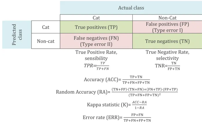
This step includes the change of some hyperparameters of the classifier, or a change in the algorithm, in order to reduce the amount of errors. A process called cross validation is commonly used for this purpose: the trainset is divided into complementary subsets, on which to separately run the model with different hyperparameters, testing it on the remaining parts. The model that performs the best is trained over the whole trainset and the generalized errors are measured on the test set. In RF classifier the cross validation is somehow included already in the algorithm itself. Compared with other ML methods, the function Out-Of-Bag (OOB) uses approximately two-thirds of the training samples in the training model. The remaining samples (out-of-bag) are used to validate the model. Hence RF will not overfit the data and the OBB accuracy is an overall unbiased estimation. 2) Test and accuracy measurement. Once the machine has understood common patterns of a class, its performances are tested. The model is fed with the images of the testset (with no information on the true classification) and it tries to classify them. This process allows to understand if the model generalizes well over data that were never seen before. The programmer knows the actual class and can understand the accuracy of the model, normally expressed as confusion matrixes, as shown in Figure 9. The accuracy is higher if more objects are correctly predicted. Accuracy (ACC) is calculated as the number of all correct predictions divided by the total samples. The best accuracy is 1.0 (100%), whereas the worst is 0.0. Since ACC is not a useful metric of a classification system when there are some classes that are not equally represented, other measurements are used in addition. Kappa statistic, for example, compares the accuracy of the system to the accuracy of a random system.
Figure 9: Example of confusion matrix, over an example of identification of cat images. True Positive Rate, True Negative Rate Accuracy, K coefficient, Error rate are some commonly used metrics to identify the performance of a classification model.
1.5 Pixel based vs Parcel Based classification
Two types of classifications can be used: pixel-based and parcel-based. Pixel-based classification consists in using information from single pixels of the image to detect common patterns. This type of analysis often lead to misclassifications due to the land cover’s spectral variability, bare soil background reflectance, atmospheric effects and mixed pixels present at the boundaries between parcels. With the increasing amount of easily accessible high resolution satellite images (with pixel size smaller than the parcel area), the attention on how to pre-process images is growing. Post-classification processing is also an important step in improving the quality of classifications when using information based on single pixels (i.e. reducing “salt and pepper” effect) (Lu & Weng, 2007; Sitokonstantinou, et al., 2018; Sicre, et al., 2020). Grouping pixels into delimited objects before classification can overcome these problems. The remote sensed image is coupled with vector parcel boundaries layer. The classification is made by unifying multiple pixel information into one single list of features statistically depending on the delimited area. This process can perform a more reliable and accurate classification (Peña-Barragán, et al., 2011). Actual class Cat Non-Cat Predict ed cl ass
Cat True positives (TP) False positives (FP) (Type error I) Non-cat False negatives (FN) (Type error II) True negatives (TN)
True Positive Rate, sensibility TPR=!"!!"!" True Negative Rate, selectivity TNR=!"!!"!" Accuracy (ACC)= !"!!"!!"!!"!"!!" Random Accuracy (RA)= !"!!" ∙ !"!!" ! !"!!" ∙(!"!!") (!"!!"!!"!!")! Kappa statistic (K)= !""!!"!!!" Error rate (ERR)= !!!!"!!"!!"!"!!"
Three assumptions are made when using a parcel-based classification on multi-temporal series: • the boundaries will not change in time; • during the period of study only one crop type is grown in the parcel; • in the same parcel there will be no subdivision of the field for multiple crops. For this study, these points are considered satisfied. First, it is very unlikely that field boundaries would change in such a short period of time as two successive years. Second, crops with sufficiently long phenology have been chosen for the classification. Third, the parcels boundary layer, with which the model is built, corresponds exactly to the specified crop cultivated inside. 1.6 Study goal The goal of this study is to create a model that identifies mayor regional crop types from satellite images, and apply it to The Netherlands. The model combines time series of radar and multispectral images from Sentinel 1 and Sentinel 2 satellites, respectively. The combination of multi-sensors and multi-temporal images enhances the classification over areas with relevant cloud coverage through the year and gives more information about growth peculiarities. The groundtruth dataset comes from the Dutch Basic Registration of crop Plots (BRP). This crop-parcel-layer is an element of the Land Parcel identification System (LPIS) that the Country uses for the Common Agricultural Policy (CAP), the EU support for agricultural income. The study relies on a parcel-based classification.
The scripts are entirely implemented in the Google Earth Engine, combining one year of satellite data (from autumn 2017 to autumn 2018) in a multiband image to feed in the classifier. Standard deviation and several vegetation indexes were added in order to have more variables for each 12-day-median image composite. The processing pays particular attention to the time variability of the mean values of each field. This provides useful information both for understanding differences among crops and the variability over the phenology of the plant.
The machine-learning algorithm used in the thesis is a Random Forest Classifier. If sufficient accuracy is achieved, further application of the model on the crop in the following years will be examined.
The specificity of the study is to apply state of the art in remote sensing processes using only open source datasets and tools, over a cloud prone region. To enhance the performance, this work has also created a time series profile, able to identify similar field spectra for the same crop class throughout the agricultural year.
Providing a free crop mapping method is a valuable step not only for control and monitoring, but also for quantifying residual biomass, organize better logistic arrangements, and many other applications.
2 Study area and Data
2.1 Study area The Netherlands has a surface of 41,873 km2. It lies between 50° and 54° N in latitude, and between 3° and 8° E in longitude. The area can be considered flat, with about 26% of the country located below the sea level and 50% one meter above the sea level. The maximum altitude is 322m a.s.l. in the southeast (see Figure 10.c) (Blom-Zandstra, et al., 2009).The climate is classified as Cfb according to the Koeppen-Geiger system, indicating a mild, marine climate with warm summers and no dry season. Average yearly temperature between 1981 and 2010 span from 9.6°C in the northeast to 11.1°C in the southwest. The amount of dry days during the year is on average higher in the south than in the north, with opposite trends for the relative humidity, that is higher in winter in the north (90%) and lower in summer in the south (76%) (Koninklijk Nederlands Meteorologish Instituut, 2011). Average yearly rainfalls are mostly concentrated in the central and northern part of the country (975 mm/y). Research shows that the intensity of precipitations has increased in the last decades due to global warming (KNML, 2020). The increasing sea level (by about 2 mm/year) brings salinity stress to the soil. Together with the increase in precipitation extremes, this may cause relevant effects to the agricultural and natural systems in the medium-long period.
The country was formed by delta deposits from the Rhine and Meuse rivers. Soil moisture, shown in Figure 10.a, is correlated to the soil types (Figure 10.b) and the elevation (Figure 10.c). Clay soils will be more affected by floods while the more elevated, south-eastern, sandy soils will suffer more in the dry seasons. In particular, the annual average temperature was 10.9 °C in 2017, 11.3 °C in 2018 and 11.2 °C in 2019. These years are all within the last 6 consecutive warmest years. Precipitations were 862 mm/y, 607 mm/y and 783 mm/y, respectively. All the three last years were warmer and dryer than the climatic mean but relatively similar between them.
Figure 10: Overview of study area. a) Soil moisture (Source: ESA’s Soil Moisture and Ocean Salinity mission). b) Soil types, based on the Soil Physical Map of the Netherlands (Kroes, et al., 2018; Wosten, et al., 2013). c) Altitude in m a.s.l. (Blom-Zandstra, et al., 2009). d) Simplified basic registration of crop plots. The boundaries of the agricultural plots are based on the Agricultural Area of the Netherlands (AAN) (Source: PDOK, geoportal of the Netherlands). Even if the agricultural sector of the Netherlands has developed vertical greenhouses, more than the 50% of the total surface is still used for open cultures. a) b) c) d)
Excluding grasslands (50% of the total), the main open-air cultivated crops are maize (25%), potatoes (19%), wheat (13%), sugar beet (10%), barley (4%) and vegetables. It is interesting to insert in the list bulbs and flower fields: blooming crops have a strong fingerprint signals for remote sensors. Phenology development of plants in the region has been taken into consideration for choosing the more representative and relevant crop classes for this study. More details about major crop calendar in this territory are shown in Table 1, extrapolated from the 2018 “Water Guide Agriculture Report” by the Foundation for Applied Water Management Research in the Netherlands (STOWA). Table 1: Crop calendar for open cultures in which the growth season takes place. Crop development (green) begins after preparatory work has taken place (plowing and seeding) indicated with orange. For winter wheat and tulip, an extra long period is taken into account before crop development actually takes place, as a result of vernalization (influence of growth processes by cold). Source: (STOWA, 2018)
Nov Dec Jan Feb Mar Apr May Jun Jul Aug Sep Oct Grass Maize Sugar beet Barley, summer Potatoes, consumption Potatoes, seeds Wheat, winter Onion, sowing Tulip Lily Leeks Legend: sowing growth harvest 2.2 Materials and Data Three different sources of data have been used for this study: SAR images from Sentinel-1, MSI images from Sentinel-2, both provided by the Google Earth Engine Data Catalog, and a vectorised parcel boundary layer provided by the LPIS National system. 2.2.1 Field Data
owner of this information is the "Ministry of Economic Affairs and Climate - Netherlands Enterprise Agency", which uses it for planning the CAP.
This dataset is updated annually at the 15th of May. The user of the parcel must indicate his crop plots annually and indicate which crop is grown on the relevant plot. Every polygon is geo-localized and associated with the label of the crop type currently cultivated in the area. The total amount of parcels corresponds to about 774000 plots, divided into 312 classes, where the majority are classified like grassland (see Figure 10.d and Figure 11).
Figure 11: BRP (Basic Registration of crop plots) dataset overview.
From the BRP dataset a certain amount of crop classes was selected to build the classifier. Following the STOWA Report, it has been decided to map only the more common crop types in the country due to their higher relevance for the final crop mapping of the region. 22 classes were used: Potatoes, consumption; Potatoes, seeds; Potatoes, starch; Corn, corncob mix; Corn, energy; Corn, grain; Corn, cut; Corn, sugar; Wheat, winter; Wheat, summer; Sugar beet; Winter barley; Summer barley; Tulip, flower bulbs and tubers; Lily, bulbs and tubers; Onions, sowing; Onions, silver; Leek, winter, production; Leeks, winter, seeds and propagating material; Leek, summer, production; Leeks, summer, seeds and propagating material. All classes not interesting for this study are classified in a final class named “Others”.
2.2.2 The Google Earth Engine
Cloud-computing based calculations and computer capabilities have been improving in recent years. Big companies like Google, Amazon and Microsoft have introduced cloud-computing tools. Google, for example, provides a constantly updated catalogue of satellite imagery for cloud-computing on a global scale on the GEE (Fuyou, et al., 2019; Gorelicka, et al., 2017)
GEE is a platform for scientific analysis and visualization of geospatial datasets, for academic, non-profit, business and government users. Based on user-developed algorithms, it combines an expanding catalogue of open source satellite imagery with global-scale analysis capabilities and Google “makes it available to detect changes, map trends, and quantify differences on the Earth's surface”. (Google, 2020)
On this platform, many different dataset sources are made available. Not only pre-processed and constantly updated satellite imagery (including, but not only, the Copernicus Programme) but also products from large scale mapping validated from acknowledged institutions (e.g., global precipitation measurements, USGS National Land Cover Database, etc.). Images fed into the GEE are pre-processed to facilitate fast and efficient access.
Furthermore, in order to allow fast visualization during algorithm elaboration, pyramids of reduced-resolution tiles are created for each image and stored in the tile database. This power-of-two downscaling enables having data ready at multiple scales without significant storage overhead, and aligns with the common usage patterns in web-based mapping (Gorelicka, et al., 2017).
Very recently, increasing research studies have been built using GEE for different purposes (Carrasco, et al., 2019; Fuyou, et al., 2019). It assembles a conventional ML method and provides a visual user interface. The Earth Engine Code Editor (see Error!
Reference source not found.) is a web-based Integrated Development Environment
(IDE) for the Earth Engine JavaScript Application Programming Interface (API). Functions ready to use, and fast to understand scripts are shown and described. It allows importing and exporting of materials in the main geospatial file formats. There is an intuitive visualization board where to observe mapped results.
Figure 12: Google Earth Engine Code Editor, the Earth Engine interactive development environment. Despite of the great capability to rapidly compute tasks and to visualise results, one GEE feature has to be highlighted: scaling errors.
A given amount of computing power and of memory is assigned to each user account in order to introduce some control to the system. Although a script may be a valid JavaScript, without logical errors, and it may represent a valid set of instructions for the server in parallelizing and executing the computations, the resulting objects may be too big or take too long to compute. In this case, an error indicating that the algorithm can't be scaled is given. These errors are generally the most difficult to diagnose and to resolve. Examples of this type of error include (Google, 2019): • “Computation timed out” • “Too many concurrent aggregations” • “User memory limit exceeded” • “Internal server error” A full community of users and Earth Engine developers are very active and provide a prompt response on forums and online networks of professionals, offering support with errors, as well as many advices for reducing the development effort.
2.2.3 Sentinel1: SAR sensor
The Sentinel1 mission (see Figure 13) involves a constellation of two polar-orbiting satellites (A and B), operating day and night performing C-band (centre frequency 5.405 GHz) synthetic aperture radar imaging. This enables to acquire imagery regardless of the weather.
Figure 13: Sentinel1 satellite from Copernicus Programme. Source: ESA
The satellites flight at 693km of altitude, with a near-polar sun-synchronous orbit. Each satellite is potentially able to map the global landmasses in the Interferometric Wide (IW) swath mode once every 12 days, in a single pass (ascending or descending). The two-satellite constellation offers a 6-days exact repeat cycle at the equator. Since the orbit track spacing varies with latitude, the revisit rate is significantly greater at higher latitudes than at the equator. Over the Netherland territory it overlaps every day in some areas.
Interferometric-Wide swath mode is one of the four different operational modes of acquisition of the signal. It is the main acquisition mode over land and satisfies the majority of service requirements. It acquires data with a 250 km swath at 5 m by 20 m spatial resolution (single look, scene). The incidence angle is 20° to 45° and the polarization modes are VV, VH, HH, HV.
Radar images are built from the intensity of the backscattered signal detected by the sensor. In an active system, the sensor, which is a transceiver, radiates electromagnetic power. It exploits the phenomenon of diffusion (scattering) that occurs when an object
distribution that depends on the shape and material of the target (dielectric constant of the medium and roughness), as well as on the system parameters (e.g., polarisation). Since clouds do not affect radar acquisition, it does not need to filter data. From November 2017 to November 2018 from 113 up to 300 passages per pixel have been counted (see the histogram in Figure 14(left)). Figure 14. Number of observations from Sentinel1 (left) and Sentinel2 (right) in the year of acquisition (1st of Nov 2017-1st of Nov 2018) on the Netherlands. Each imagery absolute frequency per pixel is shown on the occurrence histogram (this representation has 300m resolution per pixel.).
The GEE collection of Sentinel-1 repository includes the processed S1 Ground Range Detected (GRD) scenes, to generate a calibrated, ortho-corrected product. The imagery is daily updated and new assets are provided by ESA (the data provider) within two days after they become available. GRD scenes have up to 10 meters resolution, 4 bands combinations (corresponding to single or dual polarization) and three instrument modes.
GEE uses the following pre-processing steps (as implemented by the Sentinel-1 Toolbox) to derive the backscattering coefficient in each pixel: thermal noise removal, radiometric calibration and terrain correction. The backscattering coefficient is converted to decibels by log scaling (σ°!"=10*log10(intensity)) because it can vary by several orders of magnitudes. The intensity of backscattering measures whether the
radiated terrain scatters the incident microwave radiation away from (dB > 0) or towards (dB < 0) the SAR sensor.
2.2.4 Sentinel2: MSI, multispectral instrument
The Copernicus Sentinel-2 mission (see Figure 15) includes a constellation of two polar-orbiting satellites placed in the same sun-synchronous orbit, phased at 180° to each other. It aims at monitoring variability in land surface conditions, and its wide swath width (290 km) and high revisit time (10 days at the equator with one satellite, and 5 days with 2 satellites under cloud-free conditions which results in 2-3 days at mid-latitudes) will support monitoring of Earth's surface changes. It systematically acquires data over land and coastal areas from latitudes between 56° S and 84° N.
Figure 15. Sentinel-2 satellite from Copernicus Programme. Source: ESA
Sentinel2 is the sharpest free satellite imagery available today. The MSI is an innovative high-resolution multispectral imager. MSI is a passive instrument: the sensor is a receiver and measures the spontaneous emission of electromagnetic energy by the observed object. It features 13 spectral bands (as shown in Figure 3) including 3 bands for atmospheric corrections, spanning from the VNIR (Visible and Near Infrared), to the SWIR featuring 4 spectral bands at 10 m, 6 bands at 20 m and 3 bands at 60 m Spatial Sampling Distance (SSD). The signal is not detectable through all the electromagnetic spectrum due to atmospheric interferences. Within the Sentinel-2 acquisition range there are two windows in the SWIR and one that includes the NIR and VIS ranges. Each of these bands have their specific proposes due to their different interaction with the medium (the spectral band specification is shortly resumed in annex 1).
The GEE Sentinel-2 imagery is provided at a pre-processing level 2A1, computed by running sen2cor. This is a processor generated by the ESA Payload Data Ground Segment and performs the conversion from the level 1C Top-of-Atmosphere (TOA) product to the orthorectified, atmospherically corrected, Surface Reflectance (level 2A-SR). Level 1C TOA comes from the precursor levels 1B, 1A and 0 (compressed raw data). These coarse previous levels are not disseminated to users but are necessary phases to elaborate the signal transmitted directly by the satellite into usable information for the final applications.
At the 2A-RS level, in addition to the bands described above, ESA provides some supplementary information as, for example, a bitmask band with cloud mask data (AQ60) (see more details in section 3.1.3).
Figure 14 (right) shows how the images are distributed on the territory per pixel (300m of resolution). In some areas there are about 60 passages along the year of the study, concentrated in the southwest, while in other parts of the country the number rises up to almost 770. These observations are affected by cloud coverage hence a filtering process has to be done before further analysis.
1 From the mid-March 2018, the Level-2A became an operational product, beginning with coverage of the
Euro-Mediterranean region. Global coverage started in December 2018.
3 Methods
The imagery analysis has been divided into five parts:
a) Filtering of the reference field data, choosing a certain amount of polygons per class, and of the satellite data (anomalous values, clouds) with the addition of further vegetation indexes.
b) Filling the gaps in the optical images and creation of an image composite, piling radar and optical images at 24-days interval along the year. c) Creation of training and test sets by by intersecting subsets of groundtruth dataset with all pixels' information of the images throughout the year. d) Training of the RF classifier. e) Evaluation of the accuracy and validation of the model. 3.1 Preliminary data processing 3.1.1 BRP dataset
In order to create a certain amount of groundtruth data, representative and not too heavy for computational work, the BRP datasets were filtered. On the GEE, a script was developed able to select from the shapefile a collection of features (“ee.FeatureCollection’’) of up to 500 polygons in each crop class, out of a total 774822 polygons. This process is commonly named “stratified sampling”. Those polygons must represent an area of more than 100m2 each, because a field size sufficiently big for pixel statistical processing is needed. The polygons are chosen in randomly selected positions and the seed changes for every class. Random sampling for spatial dataset is rather critical when classification approaches are involved. The closer the observations are located to each other, the more similar they are. This can produce overoptimistic results (overfitting) when the test set contains observations which are somewhat similar to observations in the training set. However, this is more relevant when a pixel-based classification is conduced (Schratz, 2018).
training and test polygons was than saved to be used further on in the code (Export.table.toAsset exports a FeatureCollection as an Earth Engine asset).
Due to GEE limitations of computing power and of memory (see section 2.2.2), there are several limitations on the size and shape of GEE table assets, which are computable list of features (points or polygons) containing given variables (named properties) and georeferenced geometries. These tables can be exported or imported as well as manipulate on GEE freely once they respect certain constraints: • maximum of 100 million features, • maximum of 1000 properties (columns), • maximum of 100,000 vertices for each row's geometry, • maximum of 100,000 characters per string value. Annex 2 shows the number of polygons per class fed into the classifier. 3.1.2 Sentinel1 data VV and VH dual-band cross-polarization (vertical transmitted and horizontal received) were chosen on the Interferometric Wide (IW) swath mode by Sentinel1. Another band was successively added, called the Vegetation Index (VI), (Hosseini & McNairn, 2017) in order to enhance the amount of information per pixel. Before any calculation, backscattering values were converted into the natural scale. VI is computed as: 𝑽𝑰 = 𝑽𝑽 − 𝑽𝑯 (Eq. 1) where VV is the backscatter intensity (𝜎°) of vertically transmitted and received beams, and VH is 𝜎° of vertically transmitted and horizontally received beam. Before feeding these data to the algorithm, a filter for cleaning backscattering intensity is implemented. A mask that deletes values lower than -30dB is applied, reducing some anomalies in the signal (see an example in Figure 16).
Figure 16. Example of the time variability of the backscattering signal of one pixel of a Sentinel-1 image. The yellow curve shows the approximate viewing incident angle (from 20° to 45°). The red and blue curves show VV and VH dual-band cross-polarized dB intensity.
Another cause of non-valid data is the overlaying zones among different Sentinel-1 images. While for optical images an overlapping means higher occurrence of observation, the difference of acquisition angle of radar swats can compromise the overall backscattering value. An increase of noise is expected due to non-aligned data (Fuyou, et al., 2019). A function that computes the “geometry erosion” of Sentinel1 GRD scenes, reduces this effect eliminating images' edges. In order to prepare the SAR images for the classifier, all σ° values were converted into log scale: the ML algorithm can understand better differences if values are in this format.
3.1.3 Sentinel2 data
For MSI images, the following bands were included in the analysis: B2, B3, B4, B5, B6, B7, B8, B9, B11, B12. Moreover, two other indexes, Bare Soil Index (BSI) (Wanhui, et al., 2004) and Normalized Difference Vegetation Index (NDVI) (Tucker, 1979; Hosseini & Saradjian, 2011) were added to the information of each pixel of the optical image. These indexes are largely used in remote sensing to detect and enhance anomalies in vegetation changes. NDVI (Eq. 2) is used due to its capability to determine the photosynthetic performance of plants, because healthy canopy absorbs more red light
BSI is defined as: 𝐁𝐒𝐈 = 𝐒𝐖𝐈𝐑𝟐!𝐑𝐄𝐃 !(𝐍𝐈𝐑!𝐁𝐋𝐔𝐄) 𝐒𝐖𝐈𝐑𝟐!𝐑𝐄𝐃 !(𝐍𝐈𝐑!𝐁𝐋𝐔𝐄) ), is sensitive to the water content in the soil. 𝐍𝐃𝐕𝐈 = 𝐍𝐈𝐑!𝐑𝐄𝐃𝐍𝐈𝐑!𝐑𝐄𝐃 (Eq. 2) where RED and NIR parameters correspond to intensity in B4 and B8 respectively. BSI is defined as: 𝐁𝐒𝐈 = 𝐒𝐖𝐈𝐑𝟐!𝐑𝐄𝐃 !(𝐍𝐈𝐑!𝐁𝐋𝐔𝐄) 𝐒𝐖𝐈𝐑𝟐!𝐑𝐄𝐃 !(𝐍𝐈𝐑!𝐁𝐋𝐔𝐄) (Eq. 3)
where SWIR2, RED, NIR and BLUE parameters coincide with B12, B4, B8 and B2 intensities.
As optical images are sensitive to cloud coverage, a filtering process based on thresholds on the percentage of pixel with clouds (maximum 80% per scene) was applied. Then, a cloud mask was applied to eliminate bad observations. To elaborate this mask, an artificial bitmask band (QA60, 60m of resolution) provided by GEE was used. Bitmask for QA60 (Google, 2020): • Bit 10: Opaque clouds • 0: No opaque clouds • 1: Opaque clouds present • Bit 11: Cirrus clouds • 0: No cirrus clouds • 1: Cirrus clouds present This masking method is not perfect (not all the clouds are identified and flagged on the QA60 band) and many developers are focussing now on elaborating models able to perform more precise cloud detection. For the purposes of this work it has been decided to not investigate further on this topic, using instead the solution provided directly by GEE at a 2A-SR level of pre-processing.
3.2 Multitemporal analysis: gap filling (spatial and temporal filling)
A multitemporal series of images was created in order to build the complete list of information to associate to every polygon. The 12-day composite is a stack of images
where each of them is created by statistically associating values in a 24-days acquisition period (12 days before and after the measuring day). Every pixel should have at least 2 radar and 1 optical acquisition per sample in clear conditions.
In this study, the median values of every band of every pixel, in addition to their standard deviation, were employed. Moving median values are more recommended than mean values for remote sensing. Statistically, the moving average is optimal for recovering the underlying trend of the time series when the fluctuations about the trend are normally distributed. However, if the fluctuations are assumed to be Laplace distributed2, the moving median is statistically better. Simple statistics of time series are commonly used, because representative values can be calculated regardless of the length of the series or the lack of complete data (Fuyou, et al., 2019).
The operation on GEE for the median applied over the image collection of every moving 24 days sampling period is ee.imageCollection.median(). It reduces an image collection by calculating the median of all values at each pixel across the stack of all matching bands. Bands are matched by name.
In order to have full coverage for every pixel of all multi-sensor images some gap filling was applied. For all the Sentinel-2 data, which were masked due to cloud presence, a mosaicking procedure was implemented. As explained in Figure 17, when an image is masked by clouds, it is substituted with a patch, recovering the lack of data for that image. The patch is created by using the median values of a longer period, 80 days. Empirical tests suggested that 80 days are sufficient to have a good coverage over the territory: shorter periods would have caused lack of information in cloudy conditions. Obviously, this method allows gap filling (spatial and temporal) when periods of cloud coverage (detected with the frequency of satellite passages) are not longer than 80 days.
2 Laplace distribution represents the maximum entropy probability distribution. According to
the principle of maximum entropy, if nothing is known about a distribution except that it belongs to a certain class (usually defined in terms of specified properties or measures), then the distribution with the largest entropy should be chosen as the least-informative default. The motivation is twofold: first, maximizing entropy minimizes the amount of prior information built into the distribution; second, many physical systems tend to move towards maximal entropy configurations over time. Source: (Lawrence, 2013 ).
Figure 17: Gap filling method over long-lasting clouds for producing the time-series image composite. The GEE function .mosaic() allows merging patches of different overlapping images over the masked area. Once all the gaps are filled, standard deviation bands were added to the list. Overall, the image composite is made up with 31 images (one every 12 days) in 30 bands, derived by the optical and the radar sensors. In Figure 18, the name of all the bands are listed. The classification is done on a matrix where every “image” contains all the time series information of each band (median values of the 12-day composite) spatially averaged over all pixel contained in each crop field (parcel-based classification) and the type of cultivation information (the label on which the classifier is trained and tested). Figure 18: Method of creating the dataset for the classification process. The stack of 12 days interval images composed by the 30 bands is merged into a single image. The ee.Reducer function is applied on this image. The function computes the average over pixels included in each field boundaries of the BRP layer.
The values of each pixel of all the 12-day composite are merged together in a single object with 930 bands (30 bands times 31 images), representing the variability in time and space of each parcel of the Netherland territory. Therefore, with the function
n Band name n Band name n Band name 0 B2 10 NDVI 20 B11_stdDev 1 B3 11 BSI 21 B12_stdDev 2 B4 12 B2_stdDev 22 NDVI_stdDev 3 B5 13 B3_stdDev 23 BSI_stdDev 4 B6 14 B4_stdDev 24 VV 5 B7 15 B5_stdDev 25 VH 6 B8 16 B6_stdDev 26 VI 7 B9 17 B7_stdDev 27 VV_stdDev 8 B11 18 B8_stdDev 28 VH_stdDev 9 B12 19 B9_stdDev 29 VI_stdDev
ee.Image.ReduceRegions() to every selected BRP polygon, all mean values of the pixels included in every parcel were computed for each band. This method converts a stack of images into a collection of objects (or “features” in GEE) each with a given crop class and more than 900 properties associated, for exporting into a local cloud repository. Finally, polygons boundaries were rebuffered with an offset of 10m externally in order to recreate the real fields areas. This amount of information is at the limit of the computing power for a single GEE user. The largest computing time is taken by this step. 3.3 Random Forest Classifier and accuracy assessment At this stage of the analysis, despite the gap filling procedure, about 5% of polygons still appears with null properties. Too persistent cloud coverage interfered with the calculation of all bands for those areas. These were discarded, because the RFC needs a dataset where all objects have the same amount of properties. Figure 19: View of polygons subsets: training and test set. In order to train and test the classifier, the dataset (8335 objects, see Annex 2 for class grouping) was divided into a trainset and a testset (80% / 20% respectively), as shown in Figure 19. The drawing is random and proportioned to the class occurrence in order to maintain the representativeness of the territory.
The RFC can be tuned through several parameters. The most relevant for this study are the number of decision trees (set as 100), the minimum size of a terminal node (set as 10) and the choice of whether the classifier should run in out-of-bag mode (selected as true). Other parameters were left at their default value. The choice of the value of the main parameters, number of trees and number of variables in each node, which determine the running time, was done empirically monitoring the accuracy of the measurements. The value was chosen at a level above which the classification accuracy does not increase significantly. The function employed is ee.Classifier.randomForest(). This function creates a classifier, which uses the Random Forest algorithm. During training, the accuracy increases. The classifier is considered as trained when the accuracy converges. The training accuracy is computed with the confusion matrix (see section 4.4 and Figure 25). Once the classifier is ready, it is possible to validate the model with the test set, the remaining 1667 objects. Hence, another confusion matrix for the test accuracy is computed. The difference among the train and test accuracy allows understanding if there are over-fitting bias. Moreover, the K coefficient is computed to compare the accuracy of the model to the accuracy of a random system by weighting good predicted features with class abundance.
The classifier performances have been independently assessed for each class.
3.4 Summary of the workflow
The workflow of the study is summarized in Figure 20. At first, the analysis was based on data collecting and preparation, with the merging of all the images and satellite information with groundthruth data. Second, more vegetation indexes were added to the bands already available on GEE. The process of segmentation of those values to fields’ areas and analysing the spatial average of medians through time are the core part of this phase. Third, the datasets are fed into an RFC in order to build a model able to detect differences among many plant phenology. The accuracy in classifying the crop classes was then examined in order to evaluate the possibility to apply the model to year 2019. Annex 3 shows links references of the function to create the image composite and the RFC algorithm used for this study.
Figure 20: Workflow of the study. 3.5 Predictions As a further study, it has decided to test how an RFC built on the 2018 agricultural year can perform in the following year, with only radar imagery. In order to build the model, the same approach as described in previous sections has been used. 2019 images of the same period of the year, were collected. After submitting all scenes to the filtering and cleaning processes, they were intersected with all the selected groundthruth fields’ polygons, as described in the section 3.2. A new dataset of 8812 polygons, with their mean features derived from Sentinel1 images, makes up the test set. Every polygon includes 6 variables (VV, VH and VI with their standard deviations) referred in each 12-days time step from November 2018 to November 2019, for a total of 187 properties.
This new testset was fed into the RFC built, trained and tested on the previous year. Results of predicted agricultural classes were compared to BRP from 2019 in order to check the confusion matrix outcome and assess the accuracy.
Moreover, in order to investigate how much the accuracy of 2019 prediction could be affected by an earlier crop development due to temperature and precipitation anomalies, a third test was computed with a dataset built selecting radar images of the same period shifted in time two weeks back.
4 Results
4.1 Valid observations
As described previously, both SAR and MSI images needed some data filtering. Figure 21 reports the geographical distribution of all valid observations derived from the raw dataset. Figure 21 has to be compared with Figure 14, where all observations are shown. A reduced number of acquisitions per pixel is the result of the procedure described in section 3. Figure 21: Number of valid observations from Sentinel1 (left) and Sentinel2 (right) in the year of acquisition (1st of Nov 2017-1st of Nov 2018). This representation has a 300 m resolution per pixel. As expected, SAR images are in larger number than MSI ones (on average 216 and 202, before and after data filtering). The average number of optical valid occurrence is reduced from 189 to 76 after the selection process. Moreover, the coverage is not homogeneous over the full territory. The visible large diagonal stripes over both maps come from the overlapping scenes due to high latitude orbits (ascending and descending).
4.2 Time series trends, cleaned data and indexes (BSI, NDVI, VI)
After filtering anomalous observations and after creating the composite images, the trend through the year can be reconstructed. Watching a single field, for example, it is possible to see how these two satellites recognise crop development.
The NDVI, BSI, VV, VH and VI time series for a potato and a wheat field are shown in Figure 22. As a comparison, the same time series are shown in Figure 23 for urban areas and water surfaces.
The characteristic increase in NDVI during plant development, following by decrease during ripening and harvest, are well correlated with the decrease in BSI. While the crop is growing, the difference between VV and VH, represented by VI, is decreasing, while, overall, backscatter intensities have correlated trends with NDVI and BSI.
Figure 22: Upper panel: NDVI and BSI from Sentinel 2; lower panel: VV, VH and VI 𝝈° intensities from Sentinel1. Left graphs: potato field; right graphs: summer wheat field. Curves report the mean values of the field area throughout the 12-days moving median of the year from 2017/11 to 2018/11.
Figure 23: Upper panel: NDVI and BSI from Sentinel 2; lower panel: VV, VH and VI 𝝈° intensities from Sentinel1. Left graphs: urban areas; right graphs: water basins. Curves report the mean values of the field area throughout the 12-days moving median of the year from 2017/11 to 2018/11.
It is interesting to notice the differences between crops due to seasonality and to the development cycle, and the correlated behaviour of all parameters especially compared with signal response of urban areas and water basins. While the formers have a harmonic trend during time, the latters tend to stay stable and with either high or low intensity responses, especially with 𝜎° values. VH intensities are more representative for surface roughness: it is visible how urban areas and water basins do not have any variation throughout the period of study compare to the two crop fields. 4.3 Classification Figure 24 represents the 8335 randomly selected polygons of the 22 classes distributed on the Dutch territory as classified by RFC. The visualisation is done with the GEE Code Editor visualization panel. The classification outcome shows the geographical allocation of crop types: different classes are mixed together, while in some areas there are several groups of single crop type. The accuracy assessment would show if this feature could be related to field proximity or not.